Inverse Reinforcement Learning in Relational Domains - Hal

Inverse Reinforcement Learning in Relational Domains Thibaut Munzer, Bilal Piot, Matthieu Geist, Olivier Pietquin, Manuel Lopes

To cite this version: Thibaut Munzer, Bilal Piot, Matthieu Geist, Olivier Pietquin, Manuel Lopes. Inverse Reinforcement Learning in Relational Domains. International Joint Conferences on Artificial Intelligence, Jul 2015, Buenos Aires, Argentina.

HAL Id: hal-01154650 https://hal.archives-ouvertes.fr/hal-01154650 Submitted on 22 May 2015

HAL is a multi-disciplinary open access archive for the deposit and dissemination of scientific research documents, whether they are published or not. The documents may come from teaching and research institutions in France or abroad, or from public or private research centers.

L’archive ouverte pluridisciplinaire HAL, est destinée au dépôt et à la diffusion de documents scientifiques de niveau recherche, publiés ou non, émanant des établissements d’enseignement et de recherche fran¸cais ou étrangers, des laboratoires publics ou privés.

Inverse Reinforcement Learning in Relational Domains Thibaut Munzer Inria, Bordeaux Sud-Ouest, France [email protected]

Bilal Piot Matthieu Geist Univ. Lille-CRIStAL CentraleSupélec-MaLIS research group (UMR 9189)-SequeL team UMI GeorgiaTech-CNRS (UMI 2958) [email protected] [email protected]

Olivier Pietquin Univ. Lille-CRIStAL (UMR 9189)-SequeL team Institut Universitaire de France (IUF) [email protected] Abstract In this work, we introduce the first approach to the Inverse Reinforcement Learning (IRL) problem in relational domains. IRL has been used to recover a more compact representation of the expert policy leading to better generalization performances among different contexts. On the other hand, relational learning allows representing problems with a varying number of objects (potentially infinite), thus provides more generalizable representations of problems and skills. We show how these different formalisms allow one to create a new IRL algorithm for relational domains that can recover with great efficiency rewards from expert data that have strong generalization and transfer properties. We evaluate our algorithm in representative tasks and study the impact of diverse experimental conditions such as : the number of demonstrations, knowledge about the dynamics, transfer among varying dimensions of a problem, and changing dynamics.

1

Introduction

Learning control strategies or behaviors from observations is an intuitive way to learn complex skills [Schaal, 1999; Argall et al., 2009; Khardon, 1999]. When learning from observing another agent, one can aim at learning directly the behavior or, instead, the criteria behind such behavior. The former approach is usually called Imitation Learning (IL) while the latter is called Inverse Reinforcement Learning (IRL). The main advantage of IRL is the robustness of the behavior induced. It can handle different initial states and changes in world dynamics [Ng and Russell, 2000; Neu and Szepesvári, 2009]. With IRL, an explanation of the behavior is found, so the system can continue to learn online to fulfill this explanation via an online Reinforcement Learning (RL) algorithm. IRL also improves performance over learning the policy if a change in the world dynamics occurs. Indeed, in that case, the system will learn to adapt in order to achieve its goal while continuing to follow the same behavior (via Imitation Learning) would not. Being robust to dynamics mod-

Manuel Lopes Inria, Bordeaux Sud-Ouest, France [email protected]

ifications is an important property as, for instance, when a system ages its dynamics changes (e.g., the brake of a car will get worn). IRL can also offer a more compact representation of the behavior, modeled as a reward function. For instance, in a blocks world domain, the task of building a tower with all objects requires a non-trivial policy but can be described with a simple reward [Dˇzeroski et al., 2001]. This is useful when the user has to be aware of the internal state of the system, as a more compact representation is easier to understand for a human operator. With active learning, the user has to correct/advise the system. So, he has to quickly be able to determine what it should do. Human-machine collaboration is another setting where the user has to take into account the system and so, be informed of the internal state. Another approach for generalizing to different problems is to use representations that are more expressive. The use of relational learning allows one to generalize between worlds with different numbers of objects and agents. Learning to act from demonstrations in relational domains have been a research problem for a long time [Segre and DeJong, 1985; Shavlik and DeJong, 1987; Khardon, 1999; Yoon et al., 2002]. The use of relational representations is attracting even more attention due to new algorithmic developments, new problems that are inherently relational and the possibility of learning the representations from real-world data, including robotic domains [Lang and Toussaint, 2010; Lang et al., 2012]. Even though no approach to relational IRL has been proposed, the use of relational representation to learn from demonstrations have already been studied. Natarajan et al. [2011] propose to use of gradient-tree boosting [Friedman, 2001] to achieve IL in relational domains. In this work, the main contribution is to introduce the first IRL algorithm for relational domains. For this we generalize a previous approach for IRL, namely Cascaded Supervised IRL (CSI) [Klein et al., 2013], to handle relational representations. Another contribution is to augment CSI with a reward shaping step to boost performance. A third contribution is to show that using data from different domain sizes can improve transfer to unseen domain sizes.

The first section presents the Markov Decision Processes (MDP) framework and its extension for relational data. A second section reviews IRL in general and presents our contributions : the augmented CSI algorithm and the generalization to the relational domain. Finally, we present our results and the conclusions in the two last sections.

2 2.1

Relational Learning for Markov Decision Processes Markov Decision Process

The proposed approach for learning by demonstrations relies on the MDP framework. An MDP models the interactions of an agent evolving in a dynamic environment. Formally, it is a tuple MR = {S, A, R, P, γ} where S = {si }1≤i≤NS is the state space, A = {ai }1≤i≤NA is the action space, R ∈ RS×A is the reward function, γ ∈]0, 1[ is a discount factor and P ∈ ∆S×A (∆S is the set of distributions over S) is the S Markovian dynamics which gives the probability, P (s0 |s, a), to reach s0 by choosing action a in state s. A deterministic policy π ∈ AS maps each state to an action and defines the behavior of the agent. The quality function QπR ∈ RS×A for a given policy is a measure of the performance of this policy and is defined for each state-action couple (s, a) as the expected cumulative discounted reward when starting in state s, performing the action a and following the policy π afterwards. More P+∞ formally, QπR (s, a) = Eπs,a [ t=0 γ t R(st , at )], where Eπs,a is the expectation over the distribution of the admissible trajectories (s0 , a0 , s1 , π(s1 ), . . . ) obtained by executing the policy π starting from s0 = s and a0 = a. A policy π is said optimal when : 0

∀π 0 ∈ AS , ∀s ∈ S, QπR (s, π(s)) > QπR (s, π 0 (s)).

(1)

Moreover, the function called the optimal quality function, noted Q∗R ∈ RS×A and defined as Q∗R = maxπ∈AS QπR is important as each optimal policy π ∗ is greedy with respect to it [Puterman, 1994]: ∀s ∈ S, π ∗ (s) ∈ argmax Q∗R (s, a).

(2)

a∈A

In addition, it is well known [Puterman, 1994] that the optimal quality function satisfies the optimal Bellman equation: X Q∗R (s, a) = R(s, a) + γ P (s0 |s, a) max Q∗R (s0 , b). (3) s0 ∈S

b∈A

Equation (3) expresses a one-to-one relation between optimal quality functions and their reward functions [Puterman, 1994].

2.2

Relational MDP

One can derive a relational MDP that generalizes the reinforcement learning formalism for high level representations [Dˇzeroski et al., 2001]. Solutions to the planning and learning problems can be found in the literature [Kersting et al., 2004; Lang and Toussaint, 2010]. Relational representations generalize the commonly used representations in MDPs and machine learning. Instead of representing data as attribute-value

pairs, it relies on first order logical formulas. Given all objects and a set of possible relations (or predicates), data is represented by the set of logical rules that are true. Under this representation the state of the environment is the set of all atoms (grounded relations) that are true. The state of the environment can change when relational actions are applied. Actions have a different semantic than in finite MDPs. A relational action is abstract and so its application depends on choosing an object to apply it to, i.e., grounding the action. For instance, the action take(object) can be applied to different objects: take(cup) or take(box), and so leading to different effects.

2.3

Example Domain : Blocks world

We present a simple example domain that is going to be used to validate our approach. This is a classical domain that has several interesting and challenging characteristics such as the possibility of defining different tasks, the ease to visualize, the possibility of defining problems with a changing number of objects. Being a relational domain the blocks world can be defined by a set of objects, a set of predicates and a set of actions. The objects are the blocks and f loor, a surface where the blocks lie. There are six predicates: on(X, Y ) (true if object X is on object Y ), clear(X) (true if X is a cube and no object lies on him), cube(X), f loor(X), red(X) and blue(X). The blocks world offers two abstract actions move(X, Y ) and wait(). The wait() abstract action is available in every state and does not modify the state. The move(X, Y ) abstract action is defined with three rules that describe when the actions can be applied and what becomes the next state: for example, it can only be applied when both the block to grasp and the target block have no object on top of them. We can define multiple tasks in this domain but, to simplify discussions, we will consider only two and model them with rewards function: the first, called stack, is 1 when all blocks are stacked and 0 otherwise, the second one, called unstack, is 1 when all blocks are on the floor and 0 otherwise.

3

IRL in Relational Domains

ˆ that IRL is a method that tries to find a reward function R [ could explain the expert policy πE Ng and Russell, 2000; Russell, 1998]. More formally, an IRL algorithm receives as inputs a set DE of expert sampled transitions DE = (sk , ak = πE (sk ), s0k )1≤k≤NE where sk ∈ S and s0k ∼ P (.|sk , ak ) and some information about the world dynamics, for instance a set of non-expert sampled transitions DN E = (sl , al , s0l )1≤l≤NN E where sl ∈ S, al ∈ A, and ˆ for s0l ∼ P (.|sl , al ). Then the algorithm outputs a reward R which the observed expert actions are optimal. Most of IRL algorithms can be encompassed in the unifying trajectory matching framework defined by Neu and Szepesvári [2009]. These algorithms find a reward function such that trajectories following the optimal policy with respect to this reward function become close to the observed expert trajectories. Each step of the minimization thus requires an MDP to be solved so as to generate trajectories. These algorithms are for instance Policy Matching [Neu and Szepesvári, 2007] minimizing directly the distance between

the obtained policy and the expert policy or Maximum Entropy IRL [Ziebart et al., 2008] minimizing the KullbackLeibler (KL) divergence between the distribution of trajectories. Those algorithms are incremental by nature and have to solve several MDPs. On another hand, other IRL algorithms such as Structured Classification for IRL (SCIRL) [Klein et al., 2012] and Cascaded Supervised IRL (CSI) [Klein et al., 2013] avoid resolving recursively MDPs. In addition, most IRL algorithms are parametric and assume a linear parameterization of the reward. However this hypothesis do not hold for relational domains where states are logical formulas. Yet, CSI can be made non-parametric as we will demonstrate later. This, added to the fact that CSI doesn’t need several MDPs to be solved, makes him a good candidate for an IRL algorithm adapted to relational domains. After presenting the original CSI algorithm, we show how it can be improved by introducing an intermediate step. Then, a relational version is developed.

3.1

CSI

The idea behind CSI is that it is hard to define an operator that goes from demonstrations to a reward function. On the other hand, one can define operators to go from demonstrations to an optimal quality function and from an optimal quality function to the corresponding reward function. The second option can be made computationally efficient because of the link between the score function of a multi-class classifier and an optimal quality function. Indeed, given the data set DCE = (sk , ak )1≤k≤NE extracted from DE , a classification algorithm outputs a decision rule πC ∈ AS using sk as inputs and ak as labels. In the case of a Score Based Classification (SBC) algorithm, the output is a score function qC ∈ RS×A from which the decision rule πC can be inferred : ∀s ∈ S, πC (s) ∈ argmax qC (s, a). (4) a∈A

A good classifier provides a policy πC which often chooses the same action as πE , πC ≈ πE . Equation (4) is very similar to equation (2) thus by rewriting the optimal Bellman equation (3), qC can be directly interpreted as an optimal quality function Q∗RC for the reward RC defined as follows: X RC = qC (s, a) − γ P (s0 |s, a) max qC (s0 , b). (5) s0 ∈S

b∈A

Indeed, as qC verifies qC (s, a) = RC (s, a) + P γ s0 ∈S P (s0 |s, a) maxb∈A qC (s0 , b) and by the one to one relation between optimal quality functions and rewards this means that qC = Q∗RC . In addition, as πC is greedy with respect to qC , πC is then optimal with respect to RC . Thus, the expert policy πE is quasi-optimal for the reward RC as πC ≈ πE . However, RC can be computed exactly only if the dynamics P is provided. If not, we can still estimate RC by regression. For this, we assume that we have a set DN E of non-expert samples. So, we can easily construct a regression data set DR = {(si , ai ), rî }1≤i≤NRL from DE ∪ DN E = (si , ai , s0i )1≤i≤NE +NN E where rî = qC (si , ai ) − γ maxa∈A qC (s0i , a) is an unbiased estimate of RC (si , ai ). ˆ of The output of the regression algorithm is an estimate R the target reward RC .

Reward Shaping augmented CSI Regression implies projecting the data onto an hypothesis space. Given this hypothesis space some reward functions are easy to represent while other are hard or impossible due to the so-called inductive bias. There is a one-to-many relation between the space of demonstrations and the space of quality functions and a one-to-one relation between the space of quality functions and the one of reward functions. This means that there are many optimal candidates for the score based classification step among which one could choose the one that will be projected with the smallest error in the hypothesis space during regression. To improve the quality of its regression step, we propose to introduce an intermediate Reward Shaping (RS) step to CSI. Reward shaping is a technique aiming at modifying the reward shape while keeping the same optimal policy. [Ng et al., 1999] proved that ∀R ∈ RS×A , ∀t ∈ RS , qt (s, a) = Q∗R (s, a) + t(s) and Q∗R (s, a) share the same optimal policies and one can interchangeably use qt or Q∗R (or their corresponding reward function) to represent a behavior or a task. Although RS is traditionally used to guide reinforcement learning, here we propose to use it to shape the reward so that it can be more efficiently projected onto the chosen hypothesis space. In this context the purpose of RS is to find a function t∗ ∈ RS such that the expected error of the regression step is minimal. If one can define a criterion c over the reward values that represent the expected regression error (even heuristically), an optimization problem can be written: t∗ = argmin J(t), t 0 0 J(t) = c([qC (si , ai ) − γ max qC (s0i , a)](si ,ai ,s0i )∈DE ∪DN E ). a∈A

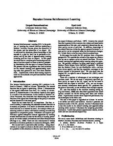
0 where qC (s, a) = qC (s, a) + t(s). The criterion c can vary substantially. For example, if the regression model is sparse the `1 -norm can be used. On the other hand, if the hypothesis space is composed of regression trees the entropy of the set of reward values is a candidate: a low entropy implies a few numbers of values which heuristically leads to a better representation with a decision tree that can only represent a finite number of values. As only a finite number of values of t change the value of c (those for which the state is present in DE or DN E ), t can be treated as a vector and standard black-box optimization tools can be used. We propose to use a simplified version of CMA-ES [Hansen et al., 2003]. Figure 1 summarizes the CSI method augmented with RS. It consists in a first step of score-based classification 1 with the set DE as input which outputs a score function qC . RS 0

(s, a) = qC (s, a) + t∗ (s) which 2 is then used to produce qC corresponds to an easier reward function to learn. From the 0 set DR constructed from DE , DN E and qC , it is possible to ˆ compute an estimate R of the reward function RC via regression . 3 Theoretical guarantees on the quality of the reward function learned via CSI are provided by Klein et al. [2013] with respect to the errors of the classification step and the regression step.

TILDE is a decision tree based regressor and therefore we choose the criteria c of the RS step to be the entropy.

4

Experiments

To validate the proposed approach, experiments have been run to (i) confirm RCSI can learn a relational reward from demonstrations, (ii) study the influence of the different parameters and (iii) show that IRL outperforms classification based imitation learning when dealing with transfer and changes in dynamics.

4.1 Figure 1: Sketch of the proposed method : CSI with reward shaping. See text for explanations.

3.2

Lifting to the relational setting

As stated earlier most algorithms for IRL in the literature rely on a parametric (propositional) representation of the MDP state. However, an IRL algorithm have to be non-parametric in order to be used in relational domains. We show here that CSI can be made non-parametric by using different supervised learners (step 1 and ) 3 than Klein et al. [2013] Relational SBC [Natarajan et al., 2011] have developed an algorithm to realize SBC in relational domains, Tree Boosted Relational Imitation Learning (TBRIL). Their algorithm is an adaptation of the gradient boosting method [Friedman, 2001] where standard decision trees have been replaced with TILDE, a relational decision trees learner (see next section). They use their method to learn a policy on relational domains from expert demonstrations but TBRIL can be more broadly used for any SBC problem in relational domains. We use TBRIL 1 as a relational SBC . 1 Relational regression TILDE [Blockeel and De Raedt, 1998] is an algorithm designed to do classification and regression over relational data. It is a decision tree learner similar to C4.5 [Quinlan, 1993]. It follows the principle of top down induction of decision trees where the dataset is recursively and greedily split by building a tree according to a criterion until all data points in one subset share the same label. The change made to handle relational data is to have first order logic tests in each node. These tests are logical formula of one atom with free variables. TILDE can be used for regression if one allows leaves to contain real numbers. To be able to represent complex functions we allows TILDE to use the count aggregator as often done in the relational learning literature [De Raedt, 2008]. Relational CSI We propose the Relational CSI algorithm (RCSI). We make three modifications to CSI : (i) use TBRIL as the SBC step

, 1 (ii) add an intermediate RS step 2 to improve the performance and (iii) use TILDE for regression step . 3 1 It should be noted that we did not use their implementation, so there are differences. In particular we do not learn a list of trees for each relational action but one list of trees for all relational actions.

Experimental setup

To test RCSI quantitatively we use the following setup. From a target reward R∗ , we compute an optimal policy π ∗ . The algorithm is given, as expert demonstrations, Nexpert trajectories starting from a random state and ending when the (first) wait action is selected. As random demonstrations, the algorithm is given Nrandom one-step trajectories starting from random states. The optimal policy π ˆ corresponding to the ˆ is then computed. As proposed by Klein learned reward R et al. [2013], the expert dataset is added to the random one to ensure that it contains important (state, action, next-state) triplets such as (goal-state, wait, goal-state). Each experiment is repeated 100 times and results are averaged. To sample the random dataset we use the following distribution, Pstate : we first draw uniformly from the different relational spatial configurations and then, for each one, uniformly from the possible groundings. The main parameters are set as follows: 10 trees of maximum depth 4 are learned by TBRIL during the SBC step 1 and the reward is learned with a tree of depth 4, which acts as a regularization parameter. Performance measure To evaluate the proposed solution we define a performance measure, the Mean Value Ratio (MVR), that measures the ratio between the expected cumulative discounted reward obtain following the learned policy (optimal policy derived from the learned reward) and following the expert one. 1000 X Qπˆ ∗ (si , π ˆ (si )) R ˆ = 1 MVR(R) , si ∼ Pstate ∗ π 1000 i=0 QR∗ (si , π ∗ (si )) Comparison to TBRIL TBRIL and RCSI have very different goals, different assumptions, and thus should not be compared directly. However, as we propose the first algorithm for IRL in relational domains, we have no baseline to compare to. TBRIL is an algorithm that has been developed to do imitation learning in relational domains and so it can inform us on what to expect from imitation in relational domains and act as a baseline. Latter we will show the advantages of estimating the reward using IRL.

4.2

Sensibility to dataset sizes

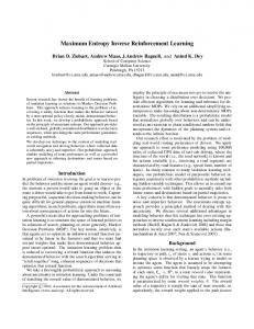
Figure 2 shows the results of using RCSI to learn the stack and unstack reward of the blocks world domain. RCSI is able of learning the reward with enough expert and random training points. This graph also shows that the RS step 2 always increases the performance of the algorithm. The setting Nrandom = 300 and Nexpert = 15 gives good results and so we will use it in the following experiments.

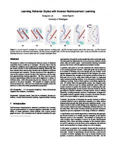
Figure 3: Performance of RCSI (and TBRIL) when different number of blocks are used for training and testing the stack (Top) and unstack (Bottom) task.

4.4

Figure 2: Performance for different amounts of training data on the stack (Top) and unstack (Bottom) task. Error bars represent standard errors.

4.3

Transfer performance

The main claim of relational learning is the ability of transferring among domain sizes. Fig. 3 shows the performance while varying the number of blocks between training and testing. For the stack reward, the graphs show almost no loss of performances due to a changing number of blocks. On the other hand, for the unstack reward, results are clearly worse when using 4, 5 or 6 blocks for training. By looking at the learned rewards, we have observed that, in most cases, one of the two following rewards is learned : one where the value is high when the number of clear is 4, 5, or 6 (depending on the number of blocks in the training set) and a second where high rewards are given when the pattern on(X, Y )∧block(Y ) cannot be matched. Both solutions are correct for a given domain size, as long as the number of blocks is the same. However, if we change the number of blocks, an ambiguity appears and only the second one stays correct. Yet, there is no reason to prefer one over the other. Moreover, for both possible rewards the expert demonstrations would be similar so the system has to choose between them based on hidden hypotheses. One way to counter this phenomenon is to use a varying number of blocks during learning. These results are shown in the last column of Fig. 3 where a reward learned with a dataset mixing demonstrations with 4 and 5 blocks successfully transfers over to 6-block problems. One can also observe that learning the reward does not perform better than directly learning the policy. This results would be surprising in a propositional domain and shows how relational representations allow to easily transfer among tasks. The advantage of IRL is shown in the following experiments.

Online learning

One interesting feature of IRL over IL is to endow the system with online learning abilities. To showcase this feature, the optimal policy of the learned reward is no more computed exactly (with value iteration) but learned online by interacting with the system using the Q-Learning algorithm [Watkins, 1989]. We define an epoch as 1000 interactions. The RCSI algorithm first learns the corresponding quality function, so we can use the results of the SBC step 1 to bootstrap the Q-Learning. Results are shown in Fig. 4. There are more efficient RL algorithms in the literature that we could have used. However, this is the proof of concept, not the better way to do online learning from the learned reward.

Figure 4: Performance of RCSI (and TBRIL) when the optimal policy is learned online.

4.5

Dynamics change

Learning the reward rather than directly the policy of the expert leads to a more robust behavior in particular when large modifications of the dynamics of the environment occur. To evaluate this ability, the dynamics of the blocks world is modified after 50 epochs. One of the blocks is made unmovable so in order to build a tower one have to stack them on top of this fixed block. The results are shown in Fig. 5. As expected, in this setup, learning the reward allows recovering a satisfying policy even after changes in the dynamics. TBRIL output, on the other hand, cannot learn from interaction and performance stays low.

Moreover, we display results of the algorithm when setting the maximum depth of the reward tree to be 2 in order to increase the regularization factor. It is done as a naive way to obtain a more general representation of the reward. It leads to better performance when the dynamics change; the learned reward transfers better to the new setting.

Figure 6: OAC of RCSI (and TBRIL) when testing in a 15 blocks world.

Figure 5: Performance of RCSI (and TBRIL) when dynamics is changed.

4.6

Big scale

It is important for an IRL algorithm to scale with the number of states. Most tasks of object manipulation are highly combinatorial, and the blocks world domain is no exception: for 5 blocks there are 501 states whereas for 15 blocks the number of states increases to 6.6 × 1013 . We evaluate RCSI in a 15 blocks world (using Nrandom = 1000). We use an alternative performance measure that is computationally more efficient, the Optimal Actions Count (OAC): ˆ = OAC(R)

1000 1 X πE 1 , 1000 i=0 ∀â∈argmaxa QRˆ (si ,a),â∈πE (si )

which is the percentage of states for which all the optimal actions for the learned reward are optimal actions for the expert. The results are shown in Fig. 6. On a 15 blocks world learning a quality function for the stack reward requires representing a very complex function, this explains that the performance for TBRIL is around 0.8; as a consequence RCSI performance is no more than 0.85. When the performance is not good enough, setting the maximum depth to 2 is too naive and prunes important features of the reward leading to low performance. For the reward unstack, optimal quality functions are trivial so TBRIL performs perfectly and RCSI performance is around 0.85. However, the performance can be improved by learning in a small domain and rely on the transfer ability of relational representations to scale to 15 blocks world. As shown in Fig. 6, the reward learned from a mixed 4 and 5 blocks world, scales very well to a 15 block world. If maximum depth is set to 2 OAC is more than 0.98 for stack and unstack rewards. Even if our goal is to learn a reward, it is also important to be able to find the corresponding optimal policy. We can do this using the prost2 planner as described by [Keller and Helmert, 2013], we search a plan in a 15 block world for the rewards learned in a mixed 4 and 5 blocks world with RCSI (maximum depth set to 2). We consider a plan to be successful if a goal state is reached and stayed in for at least 2

http://prost.informatik.uni-freiburg.de

4 time steps during the first 40 time steps. 10 plans starting from random states are computed to evaluate a learned reward function and results are averaged over 10 reward learned. For both stack and unstack, the plans are successful in more than 95% of the cases. We emphasize the strong transfer properties of mixing relational representations and IRL that allowed us to learn a reward in a small world and having such reward valid at an extremely high-dimension problem. The policy can then be found using approximated search methods [Keller and Helmert, 2013; Lang and Toussaint, 2010].

4.7

Reward learned

Learning the reward often offers a better interpretation of the behavior of the expert. Due to its compactness it is possible to visualize the reasons behind the behavior of the expert. In Fig. 7 we display the reward learned on a stack task as a tree using the prolog language. We can see that the best thing to do is to get to a state where all the blocks are stacked (there is only one clear predicate true) and wait. In any case, it it is better not to put blocks on the floor and especially when all the blocks are stacked.

Figure 7: Reward learned with RCSI on 5 blocks world.

5

Conclusions

In this paper, we have presented the first approach to IRL for relational domains. We have shown how the IRL algorithm CSI can be generalized to the relational domain. The results indicate that it is possible to learn a relational reward that explains the expert behavior. From it, a policy that matches the expert behavior can be computed. Besides generalizing the classification and regression steps in CSI, we have introduced a reward shaping step so as to reduce the regression error. Finally, we have proposed a new trans-dimensional perspective on data collection where we increase robustness to transfer over domain size by including in the training set demonstrations with different number of objects.

IRL has the advantage of more compact explanations of behaviors and increased robustness to changes in the environment dynamics. The use of relational representations allows learning policies and rewards for changing number of objects in a given domain. This shows one great strength of relational representations, and such results would not be possible in propositional or factored domains even with special feature design. Moreover, when the dynamics changes, we can see the interest of inferring the reward that allows the system to re-evaluate the expected behavior in the new conditions. In the future, we plan to apply these algorithms to more complex problems and considering the generalization of other IRL algorithms. Interesting generalizations are the active and interactive settings [Lopes et al., 2009], multi-agent domains [Natarajan et al., 2010] and consider the problem of simultaneously learn the symbolic representation and the task.

Acknowledgments This work was (partially) funded by the EU under grant agreement FP7-ICT-2013-10-610878 (3rdHand) and by the Inria-Paristech Flowers Team. We thank Marc Toussaint, Sriraam Natarajan and Kristian Kerstin for comments on this work.

References [Argall et al., 2009] Brenna D Argall, Sonia Chernova, Manuela Veloso, and Brett Browning. A survey of robot learning from demonstration. Robotics and autonomous systems, 57(5):469– 483, 2009. [Blockeel and De Raedt, 1998] Hendrik Blockeel and Luc De Raedt. Top-down induction of first-order logical decision trees. Artificial intelligence, 101(1):285–297, 1998. [De Raedt, 2008] Luc De Raedt. Logical and relational learning. Springer Science & Business Media, 2008. [Dˇzeroski et al., 2001] Saˇso Dˇzeroski, Luc De Raedt, and Kurt Driessens. Relational reinforcement learning. Machine learning, 43(1-2):7–52, 2001. [Friedman, 2001] Jerome H Friedman. Greedy function approximation: a gradient boosting machine. Annals of statistics, 29(5):1189–1232, 2001. [Hansen et al., 2003] Nikolaus Hansen, Sibylle Müller, and Petros Koumoutsakos. Reducing the time complexity of the derandomized evolution strategy with covariance matrix adaptation (cmaes). Evolutionary Computation, 11(1):1–18, 2003. [Keller and Helmert, 2013] Thomas Keller and Malte Helmert. Trial-based heuristic tree search for finite horizon mdps. In ICAPS, pages 135–143, 2013. [Kersting et al., 2004] Kristian Kersting, Martijn Van Otterlo, and Luc De Raedt. Bellman goes relational. In ICML, page 59, 2004. [Khardon, 1999] Roni Khardon. Learning action strategies for planning domains. Artificial Intelligence, 113(1):125–148, 1999. [Klein et al., 2012] Edouard Klein, Matthieu Geist, Bilal Piot, and Olivier Pietquin. Inverse reinforcement learning through structured classification. In NIPS, pages 1007–1015, 2012. [Klein et al., 2013] Edouard Klein, Bilal Piot, Matthieu Geist, and Olivier Pietquin. A cascaded supervised learning approach to inverse reinforcement learning. In Machine Learning and Knowledge Discovery in Databases (ECML/PKDD’13), pages 1–16, 2013.

[Lang and Toussaint, 2010] Tobias Lang and Marc Toussaint. Planning with noisy probabilistic relational rules. Journal of Artificial Intelligence Research, 39(1):1–49, 2010. [Lang et al., 2012] Tobias Lang, Marc Toussaint, and Kristian Kersting. Exploration in relational domains for model-based reinforcement learning. Journal of Machine Learning Research, 13(1):3725–3768, 2012. [Lopes et al., 2009] Manuel Lopes, Francisco S. Melo, and Luis Montesano. Active learning for reward estimation in inverse reinforcement learning. In Machine Learning and Knowledge Discovery in Databases (ECML/PKDD’09), 2009. [Natarajan et al., 2010] S. Natarajan, G. Kunapuli, K. Judah, P. Tadepalli, K. Kersting, and J. Shavlik. Multi-agent inverse reinforcement learning. In Machine Learning and Applications (ICMLA), 2010 Ninth International Conference on, pages 395– 400, Dec 2010. [Natarajan et al., 2011] Sriraam Natarajan, Saket Joshi, Prasad Tadepalli, Kristian Kersting, and Jude Shavlik. Imitation learning in relational domains: A functional-gradient boosting approach. In IJCAI, pages 1414–1420, 2011. [Neu and Szepesvári, 2007] Gergely Neu and Csaba Szepesvári. Apprenticeship learning using inverse reinforcement learning and gradient methods. In UAI, pages 295–302, 2007. [Neu and Szepesvári, 2009] Gergely Neu and Csaba Szepesvári. Training parsers by inverse reinforcement learning. Machine learning, 77(2-3):303–337, 2009. [Ng and Russell, 2000] Andrew Y Ng and Stuart J Russell. Algorithms for inverse reinforcement learning. In ICML, pages 663– 670, 2000. [Ng et al., 1999] Andrew Y Ng, Daishi Harada, and Stuart Russell. Policy invariance under reward transformations: Theory and application to reward shaping. In ICML, pages 278–287, 1999. [Puterman, 1994] Martin L Puterman. Markov Decision Processes: Discrete Stochastic Dynamic Programming. John Wiley & Sons, 1994. [Quinlan, 1993] J Ross Quinlan. C4. 5: Programs for Machine Learning. Morgan Kaufmann, 1993. [Russell, 1998] Stuart Russell. Learning agents for uncertain environments. In Proc. of COLT, pages 101–103, 1998. [Schaal, 1999] Stefan Schaal. Is imitation learning the route to humanoid robots? Trends in cognitive sciences, 3(6):233–242, 1999. [Segre and DeJong, 1985] Alberto Segre and Gerald F DeJong. Explanation-based manipulator learning: Acquisition of planning ability through observation. In Proc. of ICRA, pages 555–560, 1985. [Shavlik and DeJong, 1987] Jude W Shavlik and Gerald F DeJong. Bagger: an ebl system that extends and generalizes explanations. In Proc. of AAAI, pages 516–520, 1987. [Watkins, 1989] Christopher J C H Watkins. Learning from delayed rewards. PhD thesis, University of Cambridge England, 1989. [Yoon et al., 2002] Sungwook Yoon, Alan Fern, and Robert Givan. Inductive policy selection for first-order mdps. In Proc. of UAI, pages 568–576, 2002. [Ziebart et al., 2008] Brian D Ziebart, Andrew L Maas, J Andrew Bagnell, and Anind K Dey. Maximum entropy inverse reinforcement learning. In Proc. of of AAAI, pages 1433–1438, 2008.