Inverse Volume Rendering Approach to 3D ... - CiteSeerX

Inverse Volume Rendering Approach to 3D Reconstruction from Multiple Images Shuntaro Yamazaki, Masaaki Mochimaru, and Takeo Kanade Digital Human Research Center, AIST, Water Front 3F, 2-41-6, Aomi, Koto-ku, Tokyo 135-0064, JAPAN {shun-yamazaki,m-mochimaru,t.kanade}@aist.go.jp http://www.dh.aist.go.jp

Abstract. This paper presents a method of image-based 3D modeling for intricately-shaped objects, such as a fur, tree leaves and human hair. We formulate the imaging process of these small geometric structures as volume rendering followed by image matting, and prove that the inverse problem can be solved by reducing the nonlinear equations to a large linear system. This estimation, which we call inverse volume rendering, can be performed efficiently through expectation maximization method, even when the linear system is under-constrained owing to data sparseness. We reconstruct object shape by a set of coarse voxels that can model the spatial occupancy inside each voxel. Experimental results show that intricately-shaped objects can successfully be modeled by our proposed method, and the original and other novel view-images of the objects can be synthesized by forward volume rendering.

1

Introduction

Reconstruction of 3D scene information from multiple view-images is a major research topic in computer vision. Most of the existing methods of scene reconstruction attempt to create a model of the object as a solid, using boundary representation. Many real objects, however, have extremely intricate shapes, such as human hair and fur, on the surface. It is therefore difficult to represent their geometry using boundary-based representation. It is difficult to model intricately-shaped objects for two reasons. Firstly, the boundary-based shape representation is not suitable for such objects as human hair. Secondly, the resolution of optical sensors, such as Charge-Coupled Devices (CCD), is usually much lower than that of object geometry. Hence, it is inherently impossible to reconstruct complete geometry from given images. Although it is difficult to capture and reconstruct intricate shape on the object surface, the captured image can preserve the appearance of these objects in sufficient quality. This fact implies that photorealistic view can be synthesized from a reconstructed model even if the resolution of the model is not as high as that of object shape. In this paper, we propose a method of volumetric scene reconstruction using the voxels that model the spatial occupancy and color of the object. In practice,

the spatial occupancy is stored in the voxel as α value (opacity), and the synthetic view images are generated through conventional volume rendering techniques.

2 2.1

Related Work Multi-view reconstruction

The research on the method of 3D scene reconstruction from multiple viewimages has a rich history. Here we briefly describe the related work. One of the first attempts for image-based modeling of 3D scene in computer vision is two-view stereo reconstruction [1]. Okutomi et al. [2] extended the conventional two-view stereo reconstruction into the multiple-view problem and achieved convincing results. Kang et al. [3] discussed a method of multi-view stereo reconstruction from images with large occlusions. These methods are designed to reconstruct depth maps from particular viewpoints. Hence, they are not suitable for full 3D scene reconstruction from images obtained from multiple surrounding cameras. Visual hull reconstruction [?] is another approach to 3D scene reconstruction from multiple view-images. The algorithm does not need to solve the correspondence problem. Instead, it simply calculates the convex hull of silhouettes in all view images. While the visual hull method works robustly when cameras surround the object, a concave object cannot be reconstructed using silhouettes alone. This problem was solved by Seitz et al. [4] in the voxel coloring method. The original voxel coloring has a limitation on the location of input view images, which is overcome in the space carving method proposed by Kutulakos et al. [5] The opacity hull [6] method proposed by Matusik et al. is another approach to this problem. They simply use a visual hull model as an rough geometric proxy, and map opacity images using view-dependent texture mapping. This method avoids the difficulty in geometric reconstruction, but requires a lot of input images to achieve photorealistic rendering. Our proposed method is inspired by the space carving method, but has been extended so that it can deal with intricate shape within a framework of voxel modeling. Specifically, the geometrical structure within a voxel is represented as its spatial occupancy. Our method is similar to Roxels method [7] in that both can reconstruct spatial occupancy/opacity of voxels from images. The convergence of the Roxels method, however, is not proven, and the method cannot reconstruct the voxels in high resolution owing to the high computational cost. 2.2

Alpha Estimation

When a scene is captured by the digital optical sensors, such as CCD, what the device can record is not the light energy of a single light ray, but the averaged radiance incoming from a finite space in the scene. If a part of an object is observable from a single device cell, the recorded radiance is the combination of radiance coming from the corresponding foreground and background.

Alpha estimation is the process that decomposes an RGB color Cp of each image pixel into three components: foreground color Fp , background color Bp , and foreground opacity Ap . The relationship between the variables can be described by matting equation. Cp = Fp + (1 − Ap )Bp . (1) The foreground opacity, or simply, opacity Ap ∈ [0, 1] represents the contribution of the foreground object color to the pixel. When the background color in the images is controllable, we can separate these three components perfectly by capturing two images with different background colors and computing Fp and Ap which are common in the images [8]. The natural image matting methods [9– 11] can solve this problem even when the background cannot be controlled and only one image is available.

3 3.1

Inverse Volume Rendering Assumption and Preprocess

In this paper, the scene is assumed to be static and the surface reflection follows the Lambertian law. Under this assumption, the radiance emanating from the scene can be observed as a single color. Our proposed method deals with the scene composed of foreground object O, which we are interested in, and background B, which should be removed in the modeling process. The background component is removed beforehand by an appropriate method of alpha estimation described in Section 2.2. The input to our modeling algorithm is a set of color images taken at Nview different viewpoints. The accuracy of reconstruction and robustness to noise and other factors not modeled in our assumption can be increased by using as many images as possible. About 30 images uniformly distributed on the upper hemisphere surrounding O could achieve good reconstruction in our experiments. Both intrinsic and extrinsic camera parameters are supposed to be known. The output from our algorithm is a set of voxels vi which has both RGB color ci and occupancy αi . 3.2

Volume Rendering Equation

When the interest object O is captured and digitized into images by CCD, the intensity of pixel color Cp is in proportion to the sum of radiance emanating from the surfaces within a frustum spanning between the scene and the device cell. At each depth along viewing rays in the frustum, the transferred radiance is the sum of those emanating at the point (Sf ) and those coming from the behind (Sb ). Hence, the pixel colors in input images can be described by the following volume rendering equation [12]. ∑

Cp = i∈{along

a viewing ray}

ci αi

i ∏ j=0

(1 − αj ),

(2)

ci represents the radiance coming from light sources and reflected on the scene object at the depth i along viewing rays. αi ∈ [0, 1] is the ratio by which the object located at i occludes others behind it. Thus, this ratio α can be regarded as equivalent to the spatial occupancy of the foreground object at the location. Supposing that ci and αi are view-independent, they can be parameterized by the location in 3D space. We voxelize the 3D space and assign ci and αi to each voxel.

3.3

Matting Equation

First the background components observed in input images are removed from each image pixel Cp , which is combination of radiance transferred from the foreground object and the background scene. This process is essential in order to associate each voxel’s values ci and αi with pixel intensity Cp to create a 3D model of the object from the observed images. Suppose that a voxel grid spreads infinitely in 3D space. Then, we can define the mapping between the voxel coordinate (x, y, z) and the 1D coordinate s along viewing rays. For each viewing ray that goes through the foreground object O, there is a position that separates O and background B. Dividing the 1D ray coordinate into the front and back parts, equation (2) is rewritten in Cp = Fp + (1 − Ap )Bp ,

(3)

where ∏

Ap = 1 −

(1 − αk )

(4)

k∈f ront

Fp =

∑

ci αi

i∈f ront

Bp =

∑ i∈back

ci αi

i ∏

(1 − αj )

(5)

j=0 i ∏

(1 − αj ).

(6)

j∈back

Intuitively, Ap is the contribution of the spatial occupancy of voxels along a viewing ray to an image pixel, Fp is the contribution of accumulated colors of the voxels, and Bp is the background color. Compared with equation (1), it turns out that equation (3) is equivalent to the matting equation. The values Ap and Fp can be estimated from Cp before modeling voxels, by one of several methods of alpha estimation introduced in Section 2.2. Once the foreground components Ap and Fp in input images is associated with the voxel values ci and αi , we can estimate voxel values using equation (4) and equation (5) as constraints. We refer to the estimation of 3D voxel values from 3D pixels values composed of foreground components as inverse volume rendering.

3.4

Derivation of Constraints

We reconstruct the color ci and spatial occupancy αi of voxels from the accumulated color Fp and occupancy Ap of image pixels in the following two-step procedure. In the first step, we reconstruct only the voxel occupancy αi using foreground opacity Ap . Taking the logarithm of equation (4) for each Ap ̸= 1 and replacing opacity with transparency as Tp = 1−Ap and ti = 1−αi , we obtain the following equation. ∑ log(Tp ) = log(ti ) (7) i

Since log(Tp ) have already been estimated in preprocess, and therefore are regarded as constants, equation (7) comes down to a simple linear system in which log(ti ) are unknowns. In the second step, we then reconstruct voxel color ci from foreground color Fp . Now, the spatial occupancy αi has been reconstructed in the first step. Thus, equation (4) can be reduced again into a linear system Fp =

i ] ∑ [ ∏ αi (1 − αj ) ci i∈f ront

(8)

j=0

[ ] where . . . and Fp are constants, and ci are the unknowns that we want to estimate.

4 4.1

Implementation Iterative Back-projection based on EM

Various methods of solving linear systems have been proposed. When the coefficient matrix of the linear system is full-rank, we can solve the system either by using a direct method such as the Gauss-Jordan elimination, or an iterative method such as the conjugate gradient method. If the system is either under- or over-constrained, the solution that maximizes the certain likelihood measure is estimated, for instance, by singular value decomposition. Our linear system, however, cannot be solved directly by these conventional methods owing to the gigantic size of the system. The number of unknowns in equation (7) and equation (8) is equivalent to the number of voxels that increases in a cubic order. On the other hand, the number of equations in the linear system is roughly equal to the number of image pixels. Thus, the computational cost of our problem can be extremely high. It is also the case that the coefficient matrix cannot be stored in the limited working memory of a standard computer. In order to overcome these difficulties, we propose an algorithm that can solve such a gigantic linear system within a framework of the EM (Expectation Maximization) method [13]. This algorithm starts with an initial estimation of the solution, and iteratively improves the solution through the maximization of

an objective function. The algorithm can improve the solution monotonically, and can reach the global optimum. The EM estimation is composed of two steps, namely, E-step and M-step. In the E-step, the expectation of certain probabilistic phenomena is calculated using the current estimation of parameters. In the M-step, the parameters are modified so that the expectation is maximized. Repeating E-step and M-step alternatively can maximize the expectation function even when some parameters cannot be measured directly. The parameters that we want to estimate are the color ci and occupancy αi of voxels. The observed data that we have is Fp and Ap . In the E-step of the inverse volume rendering, we simply perform forward projection of voxel values. This is equivalent to the volume rendering according to equation (2). In the M-step of the inverse volume rendering, we improve either the color or the occupancy of voxels using back-projection for each viewing ray. The expectation can be calculated as a linear combination of unknowns. Hence, the function is concave and has a single global optimum. (n) Let the n-th estimations of unknowns in a linear system be {xj }, the coefficients of the system be {ri,j }, the constants of the system be {ci }, then the n + 1-th estimation of unknowns can be obtained by (n)

(n+1)

xj

xj =∑

i ri,j

∑ i

∑

ri,j ci

j

(n)

(9)

ri,j xj

∑ (n) is the result of forward projection in the E-step, and the where j ri,j xj summation of projections with regard to ri,j ci corresponds to the result of back projection. This relationship is illustrated in Fig. 1. It is worth noting that this EM estimation is a generic framework for solving linear systems. The EM algorithm in our estimation can be accelerated by dividing the problem into several subsets. First, we divide the set of input images into several subsets. Then, the linear system is solved using one of the subsets. Once the algorithm has been converged, the linear system is solved using another subset using the previous solution as an initial estimation. This scheme is called OSEM (Ordered Subset EM) [14]. In our experiments, we made subsets by choosing four images such Fig. 1. Interpretation of the upthat the distances between their viewpoints date law in EM are as large as possible. 4.2

Shell Voxels

The voxels in which no foreground object exists (αi = 0) do not affect the estimation of other voxels along the viewing rays that pass through the empty

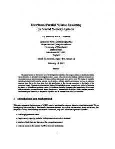
Fig. 2. Example of voxel reconstruction. (left) shell voxels in green and internal voxels in red, (center) reconstructed spatial occupancy, and (right) reconstructed color distribution.

voxel. Similarly, the voxels that are completely occupied by foreground object (α = 1) neither affect the estimation of the voxels along the viewing rays. We can reduce computational cost by just omitting the computation for these rays. After the alpha estimation for each input image has been completed, the voxels are classified into three types according to the opacities of corresponding image pixels. 1. background voxel: Ap = 0 in at least one image 2. internal voxel: Ap = 1 in all images 3. shell voxel: otherwise The classification of voxels is performed as follows. Firstly, we classify as background the voxels whose projection is completely transparent (the corresponding pixels are all Ap = 0) at least in one of input images. Secondly, we construct the visual hull [?] of completely opaque pixels (Ap = 1), and classify the voxels enclosed by the hull as internal. The rest are shell voxels. 4.3

Optimization of Voxel Traversal

In each EM estimation, a set of coefficients in the left hand of equation (7) has to be prepared. This calculation requires the voxel traversal along arbitrary viewing rays and therefore is computationally expensive. Therefore, we precompute the set of voxels along every viewing ray beforehand, and store the result into LDI structures [15] for each input pixel. We can omit the LDI entry for the pixels where Ap = 0 and Ap = 1.

5

Experimental Results

We have implemented the proposed method of inverse volume rendering and conducted some experiments on a standard PC with Pentium4 3.4GHz CPU and 2G byte main memory. Input images are captured from 36 viewpoints around

(a) object

(b) green back

(c) blue back

(d) estimated α image

Fig. 3. Multi-background matting

the object that we want to model. The size of input images are 320 × 240, and the voxel resolution is set to 643 and 1283 . 5.1

Alpha Estimation

We adopted the multi-background scheme proposed by Smith et al.[8] for alpha estimation from input images. The background color of images is controlled by a liquid crystal projector. For each viewpoint, two images with different background color, Ck1 and Ck2 in RGB color space, were taken. Let the observed image color at the same pixel be Cm1 and Cm2 respectively, then the foreground opacity Ap of the pixel can be estimated by the following equation. Ap = 1 −

(Cm1 − Cm2 ) • (Ck1 − Ck2 ) (Ck1 − Ck2 ) • (Ck1 − Ck2 )

(10)

where an operator (•) represents dot-product of RGB vectors. The foreground color Fp of the pixel is calculated as follows. ( ) Fp = Cm1 + Cm2 − (1 − Ap )(Ck1 + Ck2 ) /2 (11) An example of input images in alpha estimation and obtained alpha image is shown in Fig. 3. 5.2

Results of Volume Rendering

The reconstructed voxel model is rendered in Fig. 4. The voxels are rendered using the volume rendering equation (equation (2)) with the viewpoints not included in the input images. 5.3

Convergence

(a) input image

(b) rendered voxel model

Fig. 4. Results of volume rendering

1.2e+009

128x128x128 64x64x64

1.15e+009 SSD of reprojection error

In Fig. 6, the convergence of our proposed method is illustrated. The upper and lower rows show the process of estimating αi and ci respectively. The resolution of reconstructed voxels is 1283 . The figure indicates that the visually sufficient result can be obtained in 10 iterations.

1.1e+009

1.05e+009

1e+009

Fig. 5 is the plot of reprojection error in the EM estimation for the data shown in Fig. 6. The lines indicate the decreases in error for two different voxel resolutions. The error decreases rapidly within 5 iterations, and then gradually converges into the minimum value.

9.5e+008 5

10

15 #iterations

20

Fig. 5. Convergence

Table 1. Performance object #voxels cow mannequin

#shell vxl 643 1283 23379 185013 32531 254123

memory(byte) 643 1283 ∼256M ∼2.1G ∼510M —

time(min) 643 1283 ∼30 ∼186 ∼45 —

25

alpha voxels color voxels #iterations = 1

2

10

20

Fig. 6. Iterative optimization

5.4

Computational Cost

Table 1 shows the figures of memory usage and computational time. We have recorded these figures in the experiments using voxel resolutions of 643 and 1283 . Owing to the limitation of computer hardware, we could not conduct experiments with larger resolution. For example, reconstruction of a mannequin object with the resolution of 1283 failed because of limited memory space on 32 bit computer.

6

Discussion and Future Work

In this paper we proposed a novel method of voxel reconstruction that can deal with an object with intricate shapes such as a fur and hairs. We formulate our reconstruction process as the inverse volume rendering problem, and show how to solve it. We also present an effective implementation and conduct experiments on real objects to demonstrate the usefulness of the proposed method. In Fig. 4, we see artifacts in the fur where the spatial occupancy seems higher than the real value. The reason for this is that computing log(1 − Ap ) and log(1 − αi ) become erroneous when αi and Ap is close to 1, and therefore the small errors in alpha estimation for input image drastically affect the estimation of voxel occupancy. We implemented some measures to reduce the computational costs in the inverse volume rendering. However, the cost is still high, and therefore we cannot reconstruct the object in a proper spatial resolution. We are planning to adopt adaptive voxel structures, such as octree and k-d tree, and to extend our algorithm so that it can be executed on parallel computers.

References 1. Marr, D.C., Poggio, T.: A computational theory of human stereo vision. Proceedings of the Royal Society of London B 204 (1979) 301–328

2. Okutomi, M., Kanade, T.: A multiple-baseline stereo. IEEE Transactions on Pattern Analysis and Machine Intelligence 15 (1993) 353–363 3. Kang, S.B., Szeliski, R., Chai, J.: Handling occlusions in dense multi-view stereo. In: Proc. Computer Vision and Pattern Recognition 2001. (2001) I:103–110 4. Seitz, S.M., Dyer, C.M.: Photorealistic scene reconstrcution by voxel coloring. In: Proc. Computer Vision and Pattern Recognition ’97. (1997) 1067–1073 5. Kutulakos, K.N., Seitz, S.M.: A theory of shape by space carving. In: Proc. International Conference on Computer Vision ’99. (1999) 307–314 6. Matusik, W., Pfister, H., Ngan, A., Beardsley, P., Ziegler, R., McMillan, L.: Imagebased 3D photography using opacity hulls. In: Proc. SIGGRAPH 2002. (2002) 427–437 7. Bonet, J.S.D., Viola, P.A.: Roxels: Responsibility weighted 3d volume reconstruction. In: Proc. International Conference on Computer Vision ’99. (1999) 418–425 8. Smith, A.R., Blinn, J.F.: Blue screen matting. In: Proc. SIGGRAPH ’96. (1996) 259–268 9. Ruzon, M.A., Tomasi, C.: Alpha estimation in natural images. In: Proc. Computer Vision and Pattern Recognition 2000. (2000) 24–31 10. Chuang, Y.Y., Curless, B., Salesin, D.H., Szeliski, R.: A bayesian approach to digital matting. In: Proc. Computer Vision and Pattern Recognition 2001. Volume 2. (2001) 264–271 11. Sun, J., Jia, J., Tang, C.K., Shum, H.Y.: Poisson matting. ACM Transactions on Graphics 23 (2004) 315–321 12. Lacroute, P., Levoy, M.: Fast volume rendering using a shear-warp factorization of the viewing transformation. In: Proc. SIGGRAPH ’94. (1994) 451–458 13. Lange, K., Carson, R.: EM reconstruction algorithms for emission and transmission tomography. Journal of Computer Assisted Tomography (1984) 306–316 14. Hudson, H.M., Larkin, R.S.: Accelerated image reconstruction using ordered subsets of projection data. IEEE Transactions on Medical Imaging 13 (1994) 601–609 15. Shade, J., Gortler, S., wei He, L., Szeliski, R.: Layered depth images. In: Proc. SIGGRAPH ’98. (1998) 231–242