Inverse Volume Rendering with Material Dictionaries. Ioannis Gkioulekas. Harvard University. Shuang Zhao. Cornell University. Kavita Bala. Cornell University.
Appears in the SIGGRAPH Asia 2013 Proceedings.
Inverse Volume Rendering with Material Dictionaries Ioannis Gkioulekas Harvard University
Shuang Zhao Cornell University
Kavita Bala Cornell University
Todd Zickler Harvard University
Anat Levin Weizmann Institute
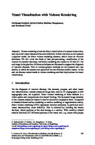
Figure 1: Acquiring scattering parameters. Left: Samples of two materials (milk, blue curacao) in glass cells used for acquisition. Middle: Samples illuminated by a trichromatic laser beam. The observed scattering pattern is used as input for our optimization. Right: Rendering of materials in natural illumination using our acquired material parameter values.
Abstract
1
Translucent materials are ubiquitous, and simulating their appearance requires accurate physical parameters. However, physicallyaccurate parameters for scattering materials are difficult to acquire. We introduce an optimization framework for measuring bulk scattering properties of homogeneous materials (phase function, scattering coefficient, and absorption coefficient) that is more accurate, and more applicable to a broad range of materials. The optimization combines stochastic gradient descent with Monte Carlo rendering and a material dictionary to invert the radiative transfer equation. It offers several advantages: (1) it does not require isolating singlescattering events; (2) it allows measuring solids and liquids that are hard to dilute; (3) it returns parameters in physically-meaningful units; and (4) it does not restrict the shape of the phase function using Henyey-Greenstein or any other low-parameter model. We evaluate our approach by creating an acquisition setup that collects images of a material slab under narrow-beam RGB illumination. We validate results by measuring prescribed nano-dispersions and showing that recovered parameters match those predicted by Lorenz-Mie theory. We also provide a table of RGB scattering parameters for some common liquids and solids, which are validated by simulating color images in novel geometric configurations that match the corresponding photographs with less than 5% error.
Scattering plays a critical role in the appearance of most materials. Much effort has been devoted to modeling and simulating its visual effects, giving us precise and efficient scattering simulation algorithms. However, these algorithms produce images that are only as accurate as the material parameters given as input. This creates a need for acquisition systems that can faithfully measure the scattering parameters of real-world materials. Collecting accurate and repeatable measurements of scattering is a significant challenge. For homogeneous materials—which is the primary topic of this paper—scattering at any particular wavelength is described by two scalar values and one angular function. The scattering coefficient σs and absorption coefficient σa represent the fractions of light that are scattered and absorbed, and the phase function p(θ) describes the angular distribution of scattering. Measurement is difficult because a sensor almost always observes the combined effects of many scattering and absorption events, and these three factors cannot be easily separated. Indeed, for deeplyscattering geometries, similarity theory [Wyman et al. 1989] proves that one can analytically derive distinct parameter-sets that nonetheless produce indistinguishable images. Most existing acquisition systems address the measurement challenge using a combination of two strategies (e.g., [Hawkins et al. 2005; Narasimhan et al. 2006; Mukaigawa et al. 2010]). First, they manipulate lighting and/or materials to isolate single-scattering effects; and second, they “regularize” the recovered scattering parameters by relying on a low-parameter phase function model, such as the Henyey-Greenstein (HG) model. These approaches can provide accurate results, but both of the employed strategies have severe limitations. The single-parameter HG model limits applicability to materials that it represents well; and this excludes some common natural materials [Gkioulekas et al. 2013]. Meanwhile, isolating single scattering relies on either: (a) diluting the sample [Hawkins et al. 2005; Narasimhan et al. 2006], which cannot be easily applied to solids or to liquids that have unknown dispersing media; or, (b) using structured lighting patterns [Mukaigawa et al. 2010], which provide only approximate isolation [Holroyd and Lawrence 2011; Gupta et al. 2011] and therefore induce errors in measured scattering parameters that are difficult to characterize.
CR Categories: I.3.7 [Computer Graphics]: Three-Dimensional Graphics and Realism—Raytracing; Keywords: scattering, inverse rendering, material dictionaries Links:
DL
PDF
Introduction
W EB
1
Appears in the SIGGRAPH Asia 2013 Proceedings. transport equation reduces to a partial differential equation [Ishimaru 1978]. The advantage of this approach is that it simplifies the inference problem, allowing efficient acquisition and rendering systems [Jensen et al. 2001; Donner and Jensen 2005] and, as demonstrated by Wang et al. [2008], the estimation of spatially-varying structure within a medium. In physics, the diffusion approximation is employed by diffusing-wave spectroscopy [Pine et al. 1990], which is used for applications such as particle sizing or the measurement of molecular weight. The diffusion approximation applies when high-order scattering is dominant, causing the phase function to be confounded with other scattering parameters [Wyman et al. 1989] and therefore reasonable to ignore. It is not appropriate for our application, where we seek material-specific phase functions that can accurately predict appearance for shapes that have arbitrary thin and thick parts.
We introduce an optimization framework that allows measuring homogeneous scattering parameters without these limitations. Our optimization undoes the effects of low-order scattering by inverting the radiative transfer equation (i.e., by inverting a random walk) using a combination of Monte Carlo rendering and stochastic gradient descent. We evaluate our optimization framework by creating a volumetric scanner that uses a camera and narrow-beam RGB sources to collect a handful of images of a material sample that resides in a box-shaped transparent glass cell (Figure 1, left). Once calibrated, this scanner provides images of low-order scattering in which the geometry is precisely known. Using these images we optimize a dictionary-based set of scattering parameters so that they produce re-rendered images that match the acquired ones. We validate our results in two ways: one, we measure prescribed dispersions of nano-scale particles whose scattering parameters can be computed using Lorenz-Mie theory and show that our recovered parameters are in close agreement; two, we re-render color images of these materials in novel lighting configurations and show that they numerically match, within 5%, the new captured images.
Single scattering and direct methods. At the other extreme are optically-thin situations, where photons scatter only once before being measured. Scattering parameters can often be measured directly in these cases, using techniques like static or dynamic light scattering [Johnson and Gabriel 1994]. For graphics, Hullin et al. [2008] use fluorescent dyes to make qualitative observations on the scattering parameters of optically thin media exhibiting mostly single scattering. Hawkins et al. [2005] use a laser to measure albedo and a tabulated phase function of a sparse homogeneous aerosol. For liquids, Narasimhan et al. [2006] successively dilute samples with water until they are sparse enough to infer from single-scattering an HG phase function. Single-scattering has also been exploited to capture time-varying and spatially-varying wisps of smoke and sparse mixing liquids [Hawkins et al. 2005; Fuchs et al. 2007; Gu et al. 2008]. All of these techniques rely on manipulating materials so that single-scattering dominates, and while dilution can be used for aerosols and some liquids, it cannot be easily applied to solids, or to liquids whose dispersing medium is unknown and significantly different from water. This limitation motivates methods for suppressing multiple scattering without dilution. Techniques for particle sizing or molecular weight, for example, exploit crosscorrelation properties of multiple temporal measurements [Pusey 1999], but these are specific to those applications and do not easily extend to our problem. For graphics, Mukaigawa et al. [2010] use high frequency lighting patterns to isolate single-scattering effects [Nayar et al. 2006], allowing direct access to the mean free path and a good initialization for an indirect (multi-scattering) optimization over an HG phase function parameter. Such lightingbased isolations of single scattering are potentially quite useful, but as discussed in the context of 3D surface reconstruction [Holroyd and Lawrence 2011; Gupta et al. 2011], they provide only approximate isolation, and there is currently no analysis of how this affects the accuracy of inferred scattering parameters.
The benefits of our approach are: (1) We can accurately measure scattering for a broader set of liquids and solids since there is no need for precisely-isolated singlescattering effects. The thickness of the glass cell can be selected appropriately for each material; but it does not need to be chosen with excessive care since our optimization succeeds for a relatively broad range of thicknesses (anywhere between 0.1 to 10 times the mean free path of the material being measured). (2) We can support general phase function measurement, and are not restricted to HG or other low parameter models, because our optimization incorporates a large material dictionary that allows phase functions to be any convex combination of hundreds of dictionary elements. These general phase functions are particularly visually important for accurate visual appearance of objects with thin features. Our contributions include: • An optimization framework to invert volumetric scattering using MC rendering and stochastic gradient descent. • An acquisition setup to acquire homogeneous material scattering properties with physically accurate parameters. • A table of RGB scattering parameters for a variety of common materials, both liquid and solid, as well as a publicly-available collection of tabulated phase functions. The availability of physically-accurate scattering parameters with general phase functions can improve simulations of translucent material appearance to better match that in the real world.
2
Low-order scattering and indirect methods. Our approach is in this category, where the goal is use moderately-thick samples to infer scattering parameters by iteratively refining them until they predict measurements that are consistent with the acquired ones (e.g., [Singer et al. 1990; Mukaigawa et al. 2010]). Most of these approaches focus like we do on homogeneous materials, since this is already very challenging. (A notable exception is Antyufeev [2000], who used regularized estimation to infer spatiallyvarying phase functions.) A common strategy in biomedical and physics domains is to simplify calculations by using planar slabs and spatially-uniform lighting that reduces the relevant scene geometry from three dimensions to two (e.g., [Chen et al. 2006; Prahl et al. 1993; McCormick and Sanchez 1981]). But this has the significant disadvantage of limiting access to angular scattering information, thereby increasing reliance on restrictive low-parameter phase function models. In contrast, our optimization applies to any geometrical configuration with any incident light field, as long as both
Related Work
Inverse radiative transport is studied in graphics, as well as in geophysical, biomedical, and chemistry domains; Bal [2009] provides a comprehensive review. Problems can be grouped into three categories, according to the ratio of the material’s mean free path—the average distance a photon travels before it is scattered—to the size of the scattering volume. We discuss these three categories in turn, and then we discuss phase function models and surface-based appearance models. Deep scattering and approximation by diffusion. Inverse problems in this category consider media that are optically-thick, so that photons scatter many times before being measured. Radiative transport is then modeled using the diffusion approximation, where the angular variation of the internal radiance is limited and the radiative
2
Appears in the SIGGRAPH Asia 2013 Proceedings. Appendix C). Complementary to the above quantities, the following two parameters are also used for describing scattering behavior: the mean free path, equal to d = 1/σt , and the albedo, equal to a = σs /σt . In the following, we will use the parameter triplet k as an interchangeable term for scattering material.
are precisely calibrated. This allows using narrow-beam illumination, which improves access to angular scattering information and allows considering a much richer space of phase function models. Phase function models. Most existing approaches to inverse radiative transfer use the single parameter Henyey-Greenstein [1941] model or other low-parameter models [Reynolds and McCormick 1980], but these can only be accurate for materials they represent well. The shape of the phase function is important for appearance, especially for objects with thin parts, and as recently shown by Gkioulekas et al. [2013], there are common materials that are not well-represented by the HG model. We avoid the restrictions of low-parameter models through the use of a phase function dictionary with hundreds of elements. This is similar in spirit to dictionary-based BRDF representations used to analyze and edit opaque scenes without being restricted to any particular analytic BRDF model (e.g., [Lawrence et al. 2006; Ben-Artzi et al. 2008]).
We consider homogeneous materials in which scattering parameters do not depend on spatial location. Scattering parameters also exhibit perceptually dominant spectral dependency [Fleming and B¨ulthoff 2005; Frisvad et al. 2007] but for notational clarity we omit wavelength dependency.
3.1
We present the operator-theoretic formulation of the RTE that we will use to setup a tractable optimization procedure for volume rendering inversion. The specific formulation we use is tailored toward our optimization algorithm, but approximations of similar nature have been considered for rendering applications [Rushmeier and Torrance 1987; Bhate and Tokuta 1992]. In the following, we consider only points x in the interior of the scattering medium; we discuss boundary conditions and other details for this formulation in the Supplementary Appendix A.
Surface reflectance fields and BSSRDF. There are a number of acquisition systems devoted to recovering surface-based descriptions of light transport through translucent objects [Debevec et al. 2000; Goesele et al. 2004; Tong et al. 2005; Peers et al. 2006; Donner et al. 2008]. These provide mappings between the input and output light fields on a specific object’s surface, and they do so without explicitly estimating all of the internal scattering parameters. They have the advantage of being very general and providing accurate appearance models for heterogeneous objects with complex shapes. Our goal is very different. We seek scattering material parameters that are independent of geometry, so that we can easily edit these materials and accurately predict their appearance when sculpted into any geometric shape.
3
Operator-theoretic formulation
We begin by considering a finite difference approximation for the directional derivative [LeVeque 2007] � � 1 ω T ∇ L (x, ω) ≈ (L (x + hω, ω) − L (x, ω)) . (3) h Defining Li (x, ω) = hQ (x − hω, ω), after simple algebraic manipulation we obtain from Equation (1) L (x, ω) = Li (x, ω) + (1 − hσt ) L (x − hω, ω) + Z � � hσs p ω T ψ L (x − hω, ψ) dµ (ψ) .
Volume light transport
Scattering occurs as light propagates through a medium and interacts with material structures. There are many volume events that cause absorption or change of propagation direction. This process has been modeled by the radiative transfer equation (RTE) [Chandrasekhar 1960; Ishimaru 1978]: � � ω T ∇ L (x, ω) = Q (x, ω) − σt L (x, ω) Z p (ω, ψ) L (x, ψ) dµ (ψ) , (1) + σs
(4)
S2
We define the following linear operator in terms of the material parameters k = {σt , σs , p (θ)}, that acts on functions on R3 × S2 Kk (L) (x, ω) , (1 − hσt ) L (x − hω, ω) Z � � + hσs p ω T ψ L (x − hω, ψ) dµ (ψ) .
(5)
S2
S2
Intuitively, the action of Kk can be viewed as a single step in the temporal propagation of a photon inside the medium. After traveling a distance of length h, the photon will transit in one of the following ways: 1) keep the same direction unaffected by the medium (probability 1−hσt ); 2) scatter towards a new direction determined by the phase function p (probability hσs ); 3) absorbed (probability h (σt − σs )). Consecutive applications of Kk describe the timeresolved random walk the photon performs as it travels through the medium.
3
where x ∈ R is a point in the interior or boundary of the scattering medium; ω, ψ ∈ S2 are points in the sphere of directions and µ is the usual spherical measure; Q (x, ω) accounts for emission from light sources; and L (x, ω) is the resulting light field radiance at every spatial location and orientation. The material is characterized by the triplet of macroscopic bulk parameters k = {σt , σs , p (θ)}. Specifically, the extinction coefficient σt controls the spatial frequency of scattering events, and the scattering coefficient σs ≤ σt the amount of light that is scattered. The difference σa = σt − σs ≥ 0 is known as the absorption coefficient and is the amount of light that is absorbed. Finally, the phase function p is a function on S2 × S2 determining the amount of light that gets scattered towards each direction ψ relative to the incident direction ω. The phase function is often assumed to be invariant to rotations of the incident direction and cylindrically symmetric; therefore, it is a function of only θ = arccos (ω · ψ) satisfying the normalization constraint Z π 2π p (θ) sin (θ) dθ = 1. (2)
Using the Kk operator, we can rewrite the RTE (4) in the form L = Li + Kk L.
(6)
Solving Equation (6) for L, we can express the light field L as the result of a radiative transfer process Rk on the input light field Li : L = Rk Li , with Rk , (I − Kk )−1 =
θ=0
(7) ∞ X
Kkj .
(8)
j=0
We also adopt this assumption in the remaining of the paper and consider only phase functions of this type (we discuss some of the technical details related to this assumption in the Supplementary
The second equality in Equation (8) follows by applying the Neumann series expansion, as it applies for the inverse of I − Kk .
3
Appears in the SIGGRAPH Asia 2013 Proceedings. (We discuss the invertibility of I − Kk in the Supplementary Appendix C.) It implies that the light field L resulting from the radiative transfer process of Equation (3) can be expressed as the sum of all orders of consecutive applications Kk to the input light field Li . That is, L corresponds to the asymptotic density of photons, when accounting for all of the intermediate positions of each photon after an arbitrary number of random walk steps. We refer to Kk as the single-step propagation operator and to Rk as the rendering operator for material k.
4.1
To better parameterize the search space in Equation (10), we use a dictionary representation for the materials. Specifically, consider a dictionary set of materials D = {kn , n = 1, . . . , N }, where kn = {σt,n , σs,n , pn (θ)}, and their corresponding single-step propagation operators {Kkn }. Then, for any weight vector π in the N -dimensional simplex ∆N , π = [πn ] ∈ RN , πn ≥ 0, n = 1, . . . , N,
The validity of the above formulation for volume light transport relies on the accuracy of the approximation in Equation (3). In the limit that h goes to zero, the operator Rk and the light field L of Equation (7) converge to the usual volume rendering operator [Jensen 2001] and the true light field inside the volume. In the Supplementary Appendix A, we discuss in detail this relationship, as well as analogies between operator Kk and Equation (8), and their counterparts derived from the volume rendering equation. As explained there, how small h needs to be depends on the extinction coefficient σt of the medium: h � ε/σt . In our experiments, we use ε = 0.01.
4
I
=S L=S
m
(I − Kk )
−1
σt,π ,
k
wm
(11)
πn σt,n ,
σs,π ,
N X
πn σs,n ,
=
(12)
n=1
PN
n=1 πn σs,n pn (θ) . PN n=1 πn σs,n
pπ (θ) ,
(13)
It is easy to see that if each pn (θ) satisfies the normalization condition of Equation (2), so does pπ (θ). In the following, we denote by K (π) and R (π) the single-step propagation (Equation (5)) and rendering (Equation (8)) operators, respectively, for the material k (π). We denote the appearance matching error of the mixing weights π as
Lm i ,
E (π) =
� ¯m 2 . S m (I − Kk )−1 Lm i −I
M X
¯m wm S m (I − K (π))−1 Lm i −I
�2
.
(14)
m=1
(9)
Then, we search for a convex combination of the material atoms in the dictionary D which best reproduces the captured images, by minimizing E (π) over π ∈ ∆N . To justify our use of convex combinations π and the mixing Equations (12)-(13), we present the following lemma. Lemma 1. For any vector π ∈ ∆N , the single-step propagation operator K(π) for the mixed material k (π) defined by Equations (12)-(13), is a convex combination of the single-step propagation operators of the individual atoms, with the exact same mixing weights, N X K (π) = πn Kkn . (15)
Given a set of illuminations {Lm M } and their correi , m = 1, . . . , � m ¯ sponding measurements I , m = 1, . . . , M , we cast the problem of inferring the material properties in an appearance matching framework: find the material parameters k that best reproduce the measurements in the least-squares sense min
N X n=1
where the sampling operator S m describes the combination of light field rays measured by the corresponding camera. The terms Lm i and S m fold in complete information about the 3D shape of the material volume, the relative light source and camera positions, as well as light interactions at the interface between the material volume and its surroundings. Modeling these light interactions involves a knowledge of the materials’ refraction indices, and an assumption there is no further scattering between the material and the camera.
M X
πn = 1,
we can represent a novel mixture material k (π) {σt,π , σs,π , pπ (θ)}, in terms of the dictionary atoms as:
We are interested in using images of an unknown material, to recover its scattering parameters k = {σt , σs , p (θ)}. Formally, we consider a known 3D shape filled with the unknown material, illuminated by calibrated light sources Lm i , and imaged by calibrated cameras to produce images I m . Using the volume scattering Equation (6), we can write m
N X n=1
Inverting volume scattering
m
Dictionary representation of materials
n=1
Proof. Denoting f = L (x − hω, ω), and using Equation (5), N X
(10)
m=1
(5)
πn Kkn (L) = (
n=1
N X
πn −h (
=1
Z +h
πn σt,π ))f
n=1
n=1
| {z }
where k is any permissible material parameter triplet {σt , σs , p (θ)}. We weight the error for each radiance mea� −1 surement with wm = max c, (I¯m )α , c, α > 0, to prevent the solution from overfitting only the brightest measurements. We selected c = 0.01 and α = 3 using the experiments on synthetic data described in Section 6.
N X
N X
|
{z
,σt
}
! � � T πn σs,n pn ω ψ f (x, ψ) dµ (ψ) .
S2 n=1
(16) For the expression of Equation (16) to be an operator of the form of Equation (5), we express the integral as: !Z �! PN N T X n=1 πn σs,n pn ω ψ πn σs,n f (x, ψ) dµ (ψ) . PN S2 n=1 πn σs,n n=1 | {z } | {z }
In the rest of this section we derive an optimization algorithm for the appearance matching problem. We express the material parameters as a convex linear combination of the material dictionary. We then differentiate the appearance matching error with respect to the mixing weights and derive an efficient optimization scheme based on stochastic gradient descent and Monte-Carlo rendering. Despite the highly non-linear problem, we show through simulations that the error surface is smooth without local minima and allows accurate reconstruction of material parameters.
,σs,π
,pπ (θ)
(17) From Equations (16) and (17), we get exactly the single-step propagation operator of the material k(π) in Equation (15).
4
Appears in the SIGGRAPH Asia 2013 Proceedings. camera sampling Sm
lighting Lm i
pπ (θ)y
pn (θ)y
Lm i −→
material sample
Lm 1 −→ S m↓
Lm 2 −→
single-step propagation Kn
full rendering R (π)
pπ (θ)y
I1m
Lm 3 −→ S m↓ full rendering R (π) I3m
Figure 2: Gradient computation (Equation (19)) for the dictionary-based appearance matching optimization problem (Equation (14)). For each pair of lighting and viewing directions, the gradient with respect to the weight of the n-th dictionary material requires computing a cascade of three rendering operations: a full volume rendering using the mixture material; then a single-step propagation using the corresponding atom material; then another full volume rendering using the mixture material. The resulting light fields are then sampled to produce the images used algebraically in Equation (19).
m 1. Render a light field Lm 1 starting from input radiance Li , and using the rendering operator R (π).
Lemma 1 shows that a convex combination of materials kn can be directly identified with a convex combination of single-step propagation operators Kkn . As a result, the objective function of the optimization problem of Equation (14) has a much simpler functional dependence on the parameters π we optimize over, allowing us to derive a tractable optimization strategy as discussed in the following subsection. This property is the key motivator for our use of the finite-difference approximation in the operator-theoretic formulation of Section 3.1. As shown in the Supplementary Appendix A deriving an analogous result from a volume rendering formulation, in contrast, requires that the extinction coefficient be known beforehand and fixed for all the atoms in dictionary D.
4.2
2. Apply the single-step propagation operator Kkn , corresponding to the n-th material kn in the dictionary D, on Lm 1 , producing a light field Lm 2 . 3. Render a light field Lm 3 , by applying the full rendering operator R (π) on Lm 2 . m 4. Apply the sampling operator S m on Lm 1 and L3 , and evaluate their product (Equation (19)).
These gradient evaluation steps are summarized in Algorithm 1, and visualized in Figure 2.
Optimization Algorithm
To minimize the appearance matching error of Equation (14), we differentiate it with respect to the mixing weights π using the following lemma: Lemma 2. For the operator K (π) defined in Equation (15), the following differentiation rule holds ∂ (I − K (π))−1 = (I − K (π)) Kkn (I − K (π)) . ∂πn
Rendering. The fact that the appearance error gradient can be expressed as a sequence of rendering steps has an important practical implication: it allows us to evaluate it efficiently using Monte-Carlo rendering techniques [Dutr´e et al. 2006]. For the first stage, in our implementation we use the traditional volume rendering operator (described in the Supplementary Appendix A), as for small enough h it produces equivalent results to the rendering operator R (π) of our finite-difference formulation. We estimate separately the direct illumination term (which depends only on the assumed known radiance sources in the scene and is easy to compute) and the indirect component. For the latter, we use a Monte-Carlo particle tracing process to estimate I1 , while simultaneously caching all intermediate particle positions in a set C1 to form an approximation of L1 . This process is described in Algorithm 3. Then the application of Kk on L1 is stochastically approximated as described in Algorithm 4: particles are uniformly sampled from C1 , propagated by h, and then either scattered or absorbed. The results are cached in a set C2 as an approximation of L2 . Finally, samples from C2 are used as sources for another full particle tracing process that directly estimates I3 , without further caching. This is performed similar to Algorithm 3, but with the initialization of x and ω in Step 2 replaced by an initialization from a particle drawn uniformly from C2 and with the caching Step 10 omitted. We discuss further details about ∂E , including handling of Fresnel the algorithm we use to render ∂π n reflection and refraction, in the Supplementary Appendix B.
(18)
This is a well-known result in the case of finite-dimensional matrices. In the Supplementary Appendix C, we provide a precise statement and proof of the lemma for the case of infinite-dimensional linear operators. Using Equations (15) and (18), we can write the gradient of E (π) with respect to each coordinate of the mixture weight vector π as M � � X ∂E ¯m (π) = 2wm S m (I − K (π))−1 Lm i −I | {z } ∂πn m=1 ,Lm 1
,Lm
·S
m
�
(I − K (π))
−1
z }|2 {� Kkn (I − K (π))−1 Lm . i | {z } ,Lm 1
|
{z
,Lm 3
}
Stochastic gradient descent. The availability of stochastic estimates of the gradient makes stochastic gradient descent (SGD) algorithms attractive for minimizing Equation (14). Similar to standard gradient descent, SGD algorithms perform iterations of steps
(19) Equation (19) is crucial for our optimization. It shows that the gradient computation simplifies to rendering and sampling operations:
5
Appears in the SIGGRAPH Asia 2013 Proceedings. Algorithm 1 ComputeGradient.
Algorithm 2 Solve appearance matching optimization problem.
N
(0)
Input: π ∈ ∆ . 1: for n = 1 to N do 2: gn ← 0. 3: for m = 1 to M do m 4: Render Lm 1 ← R (π) Li . m 5: Apply single-step propagation Lm 2 ← Kkn L1 . m 6: Render Lm ← R (π) L . 3 1 7: Sample I1m ← S m Lm 1 . m m m 8: Sample I3 ← S L3 . � 9: gn ← gn + 2wm I1m − I¯m I3m . 10: end for 11: end for 12: return g.
1: Initialize πn ← 1/N . 2: while not converged do
� � g (t) ← ComputeGradient π (t) . � � 4: π (t+1) ← P∆N π (t) − η (t) g (t) . 5: end while PT (t) 6: return π opt = T1 . t=0 π 3:
Algorithm 3 Adjoint particle tracing for computing L1 and I1 . 1: Let x0 be the location where the laser hits ∂S. 2: x ← x0 , ω ← ω L , t ← 1, C1 ← ∅. 3: while true do 4: t ← t · a. 5: Sample s from pdf p (s) = σt exp (−σt s). 6: x0 ← x + s · ω. 7: if x0 ∈ / S then 8: break 9: end if 10: Cache the particle location C1 ← C1 ∪ {(x, ω)}. 11: Let ψ 1 be the direction connecting x0 and the camera. 12: Let y 1 be the intersection of ray (x0 , ψ 1 ) and the image
proportional to the negative of the stochastic estimates of the gradient. These algorithms only require that the estimates be unbiased; even if they are otherwise noisy, there exist convergence guarantees analogous to those of standard gradient descent, with the noise variance only affecting convergence speed. This behavior has an important practical implication: we can reduce the number of particles in Monte-Carlo evaluations of the gradient, and speed computation at the cost of introducing noise to the gradient estimate. As long as the rendering algorithm is unbiased such noisy gradient estimates are valid inputs to SGD. The noise due to the reduced number of particles somewhat increases the number of iterations. However, it is still possible to reduce the number of particles quite drastically, and achieve a significant speedup in terms of overall computation time [Bottou and Bousquet 2008].
13:
14: 15: 16: 17:
As the vector π is constrained to lie on the simplex, we use projected stochastic gradient descent (PSGD). We denote by g ∈ RN consecutive noisy estimates of the gradient of E (π) obtained through Monte-Carlo rendering such that E [gn ] =
∂E (π) . ∂πn
Algorithm 4 Importance sampling for computing L2 . 1: 2: 3: 4: 5: 6: 7: 8: 9: 10: 11: 12: 13:
(20)
We use them to iterate � � π (t+1) = P∆N π (t) − η (t) g (t) ,
(21)
where P∆N denotes the Euclidean projection operator to the simplex ∆N [Duchi et al. 2008]. The step size is often chosen equal to η (t) = √ct . Though the speed of convergence depends on the proportionality constant c, in practice SGD is known to be robust to this selection. To cancel noise in individual steps, SGD returns as P its final output the average of all T iterations, π opt = T1 Tt=0 π (t) . This procedure is summarized in Algorithm 2. The optimization problem we solve is highly non-linear and essentially involves inversion of the photon random walk process. Despite the non-linear formulation, our simulations in Section 6.2 show it allows an accurate reconstruction of material parameters. While an exact proof of this property is a subject for further research, all our simulations indicate that the error surface is very smooth and does not suffer from local minima, explaining the good convergence we are able to achieve.
4.3
sensor. � v1 ← t · p ψ T1 ω · exp (−σt kx0 − y 1 k) · P0 c/A, where c is the total number of pixels on the sensor, A is the sensor’s surface area, and P0 is the source power. Add v1 to the corresponding pixel on the image sensor. Sample a direction ψ 2 according to the phase function p. x ← x0 , ω ← ψ 2 . end while
C2 ← ∅ Uniformly sample a pair (x0 , ω 0 ) ∈ C1 . x ← x0 , ω ← ω 0 . x ← x + hω. Sample u uniformly in (0, 1). if u < h (σt,k − σs,k ) then terminate end if if h (σt,k − σs,k ) < u < hσt,k then Sample a direction ψ according to the phase function pk . ω ← ψ. end if Cache the particle location C2 ← C2 ∪ {(x, ω)}.
Figure 3: Phase functions in a tent dictionary with N = 10 atoms (each atom is colored uniquely for better visualization). To be valid probability distributions on the sphere, the atoms are normalized to satisfy Equation 2, and thus have varying magnitudes. The atoms centered at 0 ◦ and π ◦ are shown cropped.
Dictionary
function component of the materials and then address the extinction and scattering components.
The dictionary-based formulation of the appearance matching problem in Equation (14) can be used with any dictionary choice1 . Our own simple dictionary is described below. We start with the phase
Phase functions. To allow the dictionary to be as general as possible, we aim to be able to express any phase function, that is, any cylindrically symmetric probability distribution on the sphere. Hence, we simply model the phase function as a piecewise linear
1 We use the term “dictionary” because the phase function sets we use can
be under- or over-complete and not strictly “bases” in the technical sense.
6
Appears in the SIGGRAPH Asia 2013 Proceedings. function of θ. Then, we can use a set of tent (triangular) functions, spaced equally over angular domain θ ∈ [0, π], to approximate it. Denoting the bins number by N and the bin spacing by θs = π/ (N − 1), we use tent functions of width 2θs and centered at points θn = (0, θs , 2θs , . . . , π). Each of the tent functions is normalized to satisfy the constraint of Equation (2). In Figure 3, we show the phase functions in a tent dictionary with N = 10. In our experiments, we use N = 200, which corresponds to a discretization step of 0.9 ◦ .
sample container frontlighting hyperspectral camera
backlighting
w
To avoid high frequency artifacts in the phase function solution we include in Equation (14) a quadratic regularization on its derivatives P 2 n (πn − πn+1 ) .
θf θo
rotation stages θb projective top view
Extinction and scattering coefficients. The definition of the atoms’ extinction and scattering coefficients should ensure that the dictionary can represent materials with a wide range of σt , σs values. We select an upper bound σt,max on the desired extinction coefficients. Note that each scattering function of the form {σt , σs , p(θ)} with 0 ≤ σt ≤ σt,max and 0 ≤ σs ≤ σt , lies on the simplex spanned by {σt,max , σt,max , p (θ)}, the purely absorptive atom {σt,max , 0, ∅}, and an atom of the form {0, 0, ∅} describing scattering-free propagation in vacuum. We use the symbol ∅ to indicate that the last two atoms are independent of phase function (the phase function is undefined for these two media). Therefore, we create a scattering dictionary including 200 atoms of the form {σt,max , σt,max , pn (θ)} with the pn (θ) defined above, plus the two purely absorptive atoms {σt,max , 0, ∅} and {0, 0, ∅}. In our experiments we set σt,max = 200 mm−1 , based on the results from Section 6.2.
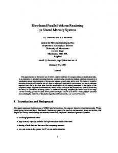
Figure 4: Setup for scattering parameter acquisition. A sample cell is illuminated by collimated beams and imaged by a camera. Rotation stages to achieve arbitrary combinations of lighting and viewing directions. Top: schematic; bottom: implementation.
Other parameterizations: Our specific choice of dictionary is aimed to represent any general phase function shape. Depending on the application, other dictionaries may be more appropriate, and some examples include: zonal spherical harmonics for lowfrequency phase functions, phase functions derived from Mie theory [Bohren and Huffman 1983; Frisvad et al. 2007] when measuring dispersions, and compact dictionaries such as a set of a few Henyey-Greenstein and von Mises-Fisher functions [Gkioulekas et al. 2013] when a simple phase function model is sufficient. A small adaptation can also allow differentiating directly with respect to the single parameter of a Henyey-Greenstein function (the average cosine). Our optimization framework is quite attractive even for retrieving such simpler phase functions, since it alleviates the need for input measurements which isolate single scattering events.
5
using Fresnel refraction and reflection laws. In our experiments, we use cells of widths w = 1, 2.5, 5, and 10 mm. Imaging and lighting. We use an approximately orthographic camera with a high magnification macro lens (4.3 ◦ subtended angle and 1 : 3 reproduction ratio) to sample the light field produced by the material volume. We use narrow (1 mm diameter) collimated beams to illuminate the sample. We use a configuration that allows illuminating either the sample surface imaged by the camera (frontlighting), or its opposite (backlighting). Through a combination of two motorized rotation stages, we can achieve different combinations of front and back lighting directions θf , θb and viewing directions θo . In our experiments, we use all possible combinations of θf , θb , θo ∈ {5 ◦ , 15 ◦ , 25 ◦ }, resulting in a set of 18 measurements per sample, 3 viewing directions times 3 frontlighting plus 3 backlighting directions.
Acquisition Setup Design
The above combination of sample shape, camera, and illumination lends itself to accurate calibration. In the Supplementary Appendix C we justify the use of collimated beams mathematically. Similar to the BRDF arguments of Ramamoorthi and Hanrahan [2001], we argue that to maximize angular information the configuration should have broadband angular frequency content, and hence be as close as possible to a delta function. The use of both frontlighting and backlighting is motivated by the understanding that a backlighting beam produces measurements dominated by high-order scattering; such measurements are intuitively useful for determining the optical thickness of the material. Conversely, frontlighting results in measurements where low-order scattering is significant, and therefore is informative for the recovery of the material phase function.
The optimization strategy described above is general enough to be applied to captured data with any geometry, as long as we can calibrate the 3D shape of the material, the relative position of the camera and light source, and the indices of refraction of the scattering material and its surroundings. Below we describe the physical acquisition setup we built, which is motivated by the simplicity of this calibration process and by some considerations related to the stability of the optimization problem. Inspiration is also drawn from analogous designs in [Jensen et al. 2001; Goesele et al. 2004; Wang et al. 2008] and physics [Johnson and Gabriel 1994]. A schematic and a photograph of our acquisition setup are shown in Figure 4. Further implementation details are provided in the Supplementary Appendix D. Geometry. We cast the material we are interested in measuring into glass cells of variable thickness w. This allows us to create box-shaped material samples whose exact shape is known with very high accuracy. Furthermore, using micron-accurate smooth glass surfaces means that transition and refraction at the various material interfaces (material and glass, glass and air) can be easily simulated
Multi-chromatic measurements. Scattering parameters vary as functions of wavelength, and this spectral dependency can create perceptually important effects in appearance [Fleming and B¨ulthoff 2005; Frisvad et al. 2007]. To capture spectral variations we use monochromatic laser light at three RGB wavelengths,
7
0
π1
1
0
π1
1
0
π1
1
1
π2 1
π2
π2
π2
1
1
0
0
1
1
π2
π1
π1
0
0
0
1
0
Experiments
x error
highly non-linear. Despite this, we almost always see in our experiments convergence to a solution that explains the measured data very well. This suggests that the error surface is fairly smooth. To provide more insight, we conduct a series of simulation experiments in which input image-sets are generated using small, artificial three-element dictionaries. Since the three mixing weights are constrained to a simplex, the set of phase functions spanned by three elements is a 2D space, allowing the entire cost surface to be visualized. For these experiments, we parameterize the 2D phase function space by the weights on the first two atoms (π1 , π2 ), and in each experiment we choose a “ground truth” phase function (π1∗ , π2∗ ) and compute for each (π1 , π2 ) the L2 -difference between input images rendered with that phase function {I m (π1 , π2 )}m=1...M and those rendered with the true one {I m (π1∗ , π2∗ )}m=1...M .
Capture and computation time
We first provide some quantitative information for the acquisition and inversion stages of our measurement pipeline. At the acquisition stage, as described in Section 5, for a single material we take measurements at three wavelengths and a set of 18 different scene configurations, for a total of 54 measurements. Each of these measurements is a high-dynamic range (HDR) image, composited from low-dynamic range images captured at 19 different exposures. In addition, for every material we measure, we capture a set of lowdynamic range calibration images. This process results in a total capture time of approximately 75 minutes per material. We provide more details about the calibration and high-dynamic range imaging procedures in the Supplementary Appendix D.
Results from six representative experiments are shown in Figure 5. Each row shows three separate experiments in which the true phase function is the same while the optical density σt differs. We find that the error surface has a clear minimum at the true value in all of these 2D experiments, and while an exact proof remains a subject for future research, the cost function appears to be very smooth and without spurious local minima, at least for these 2D problems. In the next experiment with synthetic data, we compare accuracy on absorbing materials versus scattering materials, and on materials with varying optical densities. We consider a large set of artificial materials that are combinations of: (i) σt values � sampled � logarithmically in the interval 0.01, . . . , 200 mm−1 , for a total of 21 values; (ii) σs values corresponding, for each σt , to 21 albedo values, linearly sampled between a = 0 (purely absorptive) and a = 1 (purely scattering); and (iii) a set of eight different phase functions spanning a wide range of shapes. For each artificial material we render synthetic images using geometry that matches our setup (Section 5) with a sample width of w = 1 mm. Sensor noise is an important consideration for this analysis, so we simulate image noise using photon (Poisson) noise with the parameters reported for two different commercial DSLR cameras [Hasinoff et al. 2010] (which is very large relative to the Monte Carlo rendering error). The noisy images are input to our optimization algorithm, and we measure error between the recovered parameters and the true ones. We use a tent dictionary with N = 200 atoms.
At the inversion stage, we solve the optimization problem of Section 4 on Amazon EC2 clusters of 100 nodes, with 32 computational cores and at least 20 GB of memory per node (required for the caching of intermediate light fields, as described in Section 4.2). We use the nodes to distribute the outer loop of Algorithm 1, that is, the gradient computation for each dictionary atom (for a dictionary of N = 200 atoms, each node is responsible for two atoms). The results are accumulated at a single master node, which then performs the gradient step of Algorithm 2, and the process is repeated for the number of iterations required until convergence is achieved. We found that processing one set of measurements requires approximately 200 iterations of the SGD algorithm. Overall, fitting one wavelength for a single material requires three to six hours, depending on the density of the material. We use our own C/C++ implementation, which we have optimized through experiments on synthetic data. However, computation could be reduced by further fine-tuning the various parameters involved, such as dictionary, camera spatial resolution, number of iterations, number of samples per rendering, and so on.
6.2
1
σt = 5 σt = 10 σt = 20 Figure 5: The error surface for 2D optimization problems. We consider a dictionary of three phase functions whose mixing weights lie on the simplex. The simplex is parameterized by its first two coordinates. Columns show results for three reference σt , and the rows show two different points as the correct reference in this space.
We now demonstrate and validate our approach for acquiring scattering parameters. We begin with evaluations on synthetic data aimed at understanding the characteristics of our optimization problem. We then show results on two sets of measured materials. The first is a “validation set” of carefully-constructed nano-dispersions whose scattering parameters can be computed using Lorenz-Mie theory; this set provide a means for quantitative validation. The second set consists of everyday materials that are evaluated by their ability to produce accurate rendered images for novel geometries.
6.1
π1
1
Index of refraction. To calibrate for the unknown material’s index of refraction, we use a set of additional measurements with backlighting such that θ0 = θb (corresponding to direct observation of the source in the absence of a medium). By measuring the shift in the location of the point-spread-function peak caused by refraction in these images, we can easily solve for the material index of refraction at each of the three wavelengths we use. We discuss this process in more detail in the Supplementary Appendix D. We have found our measurement procedure to be adequately accurate for our purposes, but if necessary more accurate measurements of the material index of refraction can be obtained using a refractometer. Additionally, in experiments on synthetic data, we found that small perturbations of the index of refraction (±0.1) did not affect recovered scattering parameters considerably.
6
0
π2
0
488, 533, 635 nm, and solve the optimization problem of Equation (14) independently for each wavelength.
0
Appears in the SIGGRAPH Asia 2013 Proceedings.
Figure 6 provides a summary of these experiments, by visualizing separately the relative error between the estimated and true values of (left to right): albedo a = σs /σt , extinction coefficient σt , and phase function p(θ). Each point in these tables corresponds to the percent error—averaged over the eight true phase function shapes— for distinct values of true albedo (horizontal axis) and extinction coefficient (vertical axis). These tables reveal which types of materials we can expect to measure accurately with our setup. Traveling from
Experiments with Synthetic Data
The optimization problem of Section 4 involves the inversion of a random walk process that includes multiple scattering events and is
8
Appears in the SIGGRAPH Asia 2013 Proceedings. extinction coefficient error (%)
absorptive
scattering
mean free path (log) long
short
scattering
absorptive
short
phase function error (%) 50 45 40 35 30 25 20 15 10 5 0
mean free path (log)
50 45 40 35 30 25 20 15 10 5 0
long
long
mean free path (log)
short
albedo error (%)
scattering
absorptive
100 90 80 70 60 50 40 30 20 10 0
albedo albedo albedo Figure 6: Accuracy in the recovery of material parameters. The plots show recovery errors for albedo, extinction coefficient, and mean error for phase function, as a function of different values of albedo a = σs /σt and mean free path d = 1/σt .
hand cream
left to right in these tables makes a gradual transition from purely absorbing materials to purely scattering ones. Traveling from bottom to top moves through materials of increasing optical density, with the top being materials whose mean free path is two hundred times smaller than the sample width d = 1/σt = w/200, and the bottom being materials whose mean free path is one hundred times larger than the sample width d = 1/σt = 100w.
shampoo
olive oil
robitussin
blue curacao mixed soap
whole milk mustard
The first observation—based on the large, low-error regions in the center of the tables—is that estimation is accurate for a wide range of optical densities. This is a useful fact because it means the width of the glass cell need not be chosen with excessive care. We expect very accurate results as long as the sample width is within an order of magnitude of the material’s mean free path, and we expect graceful degradation when the width extends beyond this in either direction. For extremely optically-thin materials (lower rows in table), scattering events become very rare, and images are dominated by noise. For extremely optically-thick materials (top rows), the diffusion approximation [Jensen et al. 2001] becomes applicable, and recovering both the phase function and the scattering coefficient becomes ill-posed. In practice, we simply choose the width for each material sample from a discrete set of available glass cells (1, 2.5, 5, 10 mm) so that they look reasonably translucent under natural light; see examples in Figure 7.
coffee
wine reduced milk
milk soap liquid clay
Figure 7: Measured materials in glass cells of width w = 1, 10, and 2.5 mm, from left to right. It is not necessary for all of the cell to be filled, as long as there exists a homogeneous region of size comparable to the beam diameter (e.g., hand cream).
6.3
Validation materials
It is common in graphics to evaluate measured scattering parameters by demonstrating renderings of visually plausible results. This is an important benchmark, but it does not directly assess the accuracy of the recovered physical parameters. Since our goal is to produce parameters that are faithful to the true mean free path lengths and phase functions in an absolute sense, being able to directly validate the scattering parameters is crucial. To achieve comparison to “ground truth” parameters, we capture liquid materials whose exact physical structure are known, similar to materials that are used to calibrate instruments used in a variety of domains for particle sizing or estimating molecular weight [Johnson and Gabriel 1994; Pine et al. 1990]. They are created by dispersing nano-scale spherical particles of known chemical composition into a homogeneous embedding medium of a different refractive index, using procedures that allow for very precise control of particle concentration, particle size distribution, and homogeneity. Given these parameters, Lorenz-Mie theory [Bohren and Huffman 1983; Frisvad et al. 2007] provides analytic expressions of the bulk material scattering parameters {σt , σs , p (θ)} at any wavelength.
Errors induced by extreme optical thinness and thickness at the top and bottom of these tables should be interpreted differently. If a material is excessively thin at sample width w, it is relatively easy to instead use a glass cell that is larger. This is less true for materials that are excessively dense, however, since it is physically challenging to cast materials into glass cells that are too small (w < 1 mm). Thus, in cases of extreme optical thickness, our setup will not provide material parameters that can accurately predict appearance on arbitrary geometries, but only for novel geometries at least as wide as the measured sample. As expected, we also observe large errors in the estimated phase function when materials are extremely absorptive (left column of third table in Figure 6). These errors are somewhat of a computational artifact and have a limited impact on visual appearance. They occur because the appearance of these materials is dominated by attenuation due to absorption, so very little scattering is observed and there is little discernible information about the shape of the phase function. These errors do not impact our ability to predict material appearance, however, because the phase function makes little difference. Indeed, for purely absorptive materials (left-most column) there is no scattering at all, and the phase function can be defined arbitrarily without having any effect on appearance.
We measure nanodispersions of two types. First, we measure dispersions of polystyrene spheres in water that are almost monodisperse (single particle size) and are precise enough to be traceable to NIST Standard Reference Materials. We measure three such dispersions2 , each having a 1% (w/v) concentration of particles at a different particle radius: 200, 500, or 800 nm. Second, we measure a spherical polydispersion of aluminum oxide particles (Al2 O3 ) in water3 , with an approximately known particle size distribution in 2 Nanobead 3 NanoArc
9
NIST Traceable Particle Size Standards, Polysciences, Inc. Aluminum Oxide, Nanophase Technologies Corporation.
Appears in the SIGGRAPH Asia 2013 Proceedings. the range 20 − 300 nm and mean radius of 30 nm. We use glass cells of width w = 1 mm for all of these measurements, and instead of estimating the indices of refraction from image data, we use those predicted by Lorenz-Mie theory.
photographs in these same novel configurations. For the novel configurations, we use lighting angles θf , θb ∈ {10 ◦ , 20 ◦ , 30 ◦ } and glass cells with widths w ∈ {2.5, 5 mm}. The generalization error for each material is reported as the average relative L2 image difference over the set of all novel configurations. As shown in the right two columns of Table 2, fitting errors are less than 4% and generalization errors below 5%.
The results of our measurements are shown in Table 1. In all cases, the error in the recovered parameters is less than 5%. (Note that these materials are purely scattering, so σt = σs .) The largest error occurs for the aluminum oxide material, for which the particle size distribution is known much less precisely. Figure 8-left compares the green-channel phase functions recovered by our optimization (purple curves) to the ground truth phase functions predicted by Lorenz-Mie theory (dotted orange curves). We see that the matches are extremely close. As a reference, we compare both to HenyeyGreenstein phase functions; as the single parameter g of an HG phase function is equal to its average cosine, we plot (green curves) the HG phase function that have g values that are equal to the average cosine of the ground truth phase function. We note that their shapes deviate significantly from the ground-truth. This deviation is important for appearance, particularly for objects that have thin geometry with low-order scattering, where the phase function plays an important role visually. The middle columns demonstrate this by showing captured and fit (pseudo-colored) images of the materials under frontal laser illumination at a new angle (which was not used in optimization). The rightmost column shows cross-sections of the image intensities. The deviations of the HG fits from ground-truth lead to discernible differences between the images.
Figure 9 shows the measured phase functions, each superimposed with an HG phase functions whose g-value is equal to the average cosine of the phase function we measure. Some of these phase functions are well approximated by the HG model but others, including hand cream, liquid clay, and mixed soap, are not. This set of tabulated phase functions is available at the project website. As qualitative evaluation, Figure 1-right shows an image rendered with our recovered material parameters under natural lighting. From left to right, are milk soap and glycerine soap (top and bottom, respectively), olive oil, blue curacao, and reduced milk. The soap geometry corresponds to scanned molded cubes made of the corresponding materials. We see that the recovered material parameters successfully reproduce the color variations that are critical to the translucent appearance of these materials. This is most notable in the glycerine soap, where blue wavelengths scatter first and cause a reddish glow in the middle of the object, but it is also visible on the left edge of the milk soap and the top-right corner of the milk. A high-resotion version of Figure 1 and a visualization that highlights the color variations are shown in the Supplementary Appendix E. The scene file used for this figure is available at the project website.
These experiments highlight the fact that simple, single-parameter phase function models can be insufficient for modeling the appearance of scattering materials, and it justifies our choice to fit higherdimensional phase function models.
6.4
7
Conclusions
We present an optimization framework for inverting the effect of multiple-scattering to recover scattering properties of homogeneous volumes from a handful of images. The approach does not require precise isolation of single scattering, and this enables the measurement of a broader set of materials, including both solids and liquids. The optimization also incorporates a large material dictionary and thereby avoids the restrictions of low-parameter phase function models. Our analysis and experiments show that we can recover accurate physical scattering parameters for a variety of materials.
Other materials
Next, we use our acquisition setup and optimization algorithm to measure several common materials. They can be grouped roughly into three categories: • Highly scattering liquids of varying viscosities; including mustard, shampoo, hand cream, liquid designer clay, and different types of milk.
Our current setup and optimization framework do not account for polarization or fluorescence phenomena. Polarization can be important for the appearance of materials with strongly polarizationdependent scattering properties or index of refraction (birefringence), such as crystalline materials. Experimentally, our optimization has been unable to find scattering parameters that match our setup’s images of microcrystalline wax, and this may be due to some combination of our simulator’s ignorance of polarization and our use of partially-polarized (laser plus fiber) light. Regarding fluorescence, we have verified that it has negligible impact on our measurements of the materials listed in Section 6. Our setup can be easily modified to measure the strongly fluorescent behavior of other materials, by including in addition to the hyperspectral camera a mechanism to control wavelength at the source side.
• Highly absorbing liquids with limited scattering; including coffee, robitussin, olive oil, blue curacao liquor, and red wine. • Solids that can be molded into the glass cells; such as different types of soap. By “eyeballing” each sample under natural light, we choose glass cell widths so that each sample looks reasonably translucent under ambient lighting. The results we report were captured using width w = 1 mm for materials in the first and third categories, except for glycerine soap; and w = 10 mm for the second category and glycerine soap. Photographs of samples in 1 mm, 2.5 mm, and 10 mm cells are shown in Figure 7. For each sample, we estimate the index of refraction as described in Section 5, and these range from values of 1.33 (for milk, reduced milk, milk soap, and the water soluble liquids) to 1.47 (for olive oil and glycerine).
While we proposed one possible scanning configuration, our optimization could be used to infer scattering parameters from images captured from a variety of scene geometries and incident light fields. The only requirement is that both lighting and geometry be precisely calibrated. Our setup combines the benefits of highfrequency angular lighting (for stable optimization) and precise, stable calibration (for repeatability), but it limits measurements to three wavelengths and to solids that can be cast into glass cells of thickness within an order of magnitude of the mean free path. In principle, our optimization could be applied to images of more general solid objects, but this would require enhancing our setup to also
The measured parameters are shown in Table 2. We quantitatively evaluate the quality of the recovered scattering parameters in two ways. First, we report the fitting error, which is the average L2 image difference between input images and the corresponding images rendered with the recovered parameters, normalized by the L2 -norms of the input images. Second, we compute a measure of generalization error by: i) using the recovered parameters to render laser-illumination images with different sample widths and lighting directions; and ii) comparing these simulated images to captured
10
Appears in the SIGGRAPH Asia 2013 Proceedings.
dispersion polystyrene, 200 nm polystyrene, 500 nm polystyrene, 800 nm Al2 O3 , 30 nm
R 17.220 59.082 65.757 47.341
σs predicted G B 28.363 36.517 79.557 88.626 70.438 68.589 93.389 129.870
R 17.078 58.431 66.976 48.536
σs measured G B 28.650 36.823 79.023 88.062 71.544 69.146 96.004 132.695
R 0.825 1.102 1.853 2.524
σs error (%) G B 1.012 0.838 0.671 0.636 1.570 0.812 2.800 2.175
phase function error (%) R G B 3.031 1.143 3.672 3.181 2.676 1.359 2.623 2.117 1.251 3.712 4.298 3.108
Al2 O3 , 30 nm
polystyrene, 800 nm
polystyrene, 500 nm
polystyrene, 200 nm
� Table 1: Measurements of validation materials (controlled nano-dispersions). Values for σs are reported in mm−1 . Phase function error is given as L2 difference normalized by the L2 -norm of the reference phase function. All four validation materials have negligible absorption, resulting on both the predicted and measured values for σt to agree with those we report for σs to the third decimal.
phase function
captured
dictionary fit
HG fit
cross section
Figure 8: Measurements of validation materials (controlled nano-dispersions). Left: For each material, we show for the green wavelength the theoretically predicted (dashed orange) and recovered (purple) phase functions, as well as the best Henyey-Greenstein (green) phase function fit. The recovered phase functions are in close agreement with the correct ones and the purple and orange curves tightly overlap. As another visualization, we show the images for a novel configuration: under frontal collimated laser illumination (θf = 25 ◦ , θo = 0 ◦ ). We compare our phase function and the best Henyey-Greenstein fit (images are color-mapped for better visualization). The rightmost column shows a crossection through the captured and re-rendered images for this configuration.
Acknowledgments
recover the object shape and its surface microstructure (BSDF).
We thank Henry Sarkas at Nanophase for donating material samples and calibration data. Funding by the National Science Foundation (IIS 1161564, 1012454, 1212928, and 1011919), the European Research Council, the Binational Science Foundation, Intel ICRI-CI, and Amazon Web Services in Education grant awards. Much work was performed while T. Zickler was a Feinberg Foundation Visiting Faculty Program Fellow at the Weizmann Institute.
In addition, combinations of our optimization framework with more sophisticated imaging configurations could improve the optimization’s stability and convergence rate. In particular, it may be fruitful to apply our optimization to images captured with high-frequency illumination [Mukaigawa et al. 2010], basis illumination [Ghosh et al. 2007], adaptive illumination [O’Toole and Kutulakos 2010], or transient imaging [Wu et al. 2012]. It is also possible that optimization schemes like ours will allow exploiting such imaging modalities to solve more challenging inverse problems, such as measuring heterogeneous scattering media.
References A NTYUFEEV, V. 2000. Monte Carlo method for solving inverse
11
Appears in the SIGGRAPH Asia 2013 Proceedings.
material whole milk reduced milk mustard shampoo hand cream liquid clay milk soap mixed soap glycerine soap robitussin coffee olive oil blue curacao red wine
R 100.920 57.291 16.447 8.111 20.820 37.544 7,625 3.923 0.201 0.009 0.054 0.041 0.010 0.015
σs G 105.345 62.460 18.536 9.919 32.353 48.250 8.004 4.018 0.202 0.001 0.051 0.039 0.012 0.013
B 102.768 63.757 6.457 10.575 41.798 67.949 8.557 4.351 0.221 0.001 0.049 0.012 0.021 0.011
R 0.013 0.007 0.057 0.178 0.011 0.004 0.003 0.003 0.001 0.012 0.275 0.062 0.083 0.122
σa G 0.013 0.007 0.061 0.328 0.011 0.004 0.004 0.005 0.001 0.197 0.309 0.047 0.048 0.351
B 0.041 0.024 0.451 0.439 0.012 0.005 0.015 0.013 0.002 0.234 0.406 0.353 0.011 0.402
R 0.954 0.954 0.155 0.907 0.188 0.312 0.164 0.330 0.955 0.906 0.911 0.946 0.955 0.947
first moment G B 0.963 0.946 0.957 0.942 0.173 0.351 0.882 0.874 0.247 0.265 0.442 0.512 0.167 0.155 0.322 0.316 0.949 0.943 0.977 0.980 0.899 0.906 0.954 0.975 0.973 0.979 0.975 0.977
fitting error (%) 2.0460 1.346 3.377 3.962 2.652 3.431 1.895 1.474 3.840 1.379 1.957 2.287 2.704 3.034
generalization error (%) 3.6344 2.039 4.201 4.752 3.221 4.532 2.956 3.316 3.920 3.998 2.199 3.846 4.857 3.192
Table 2: Scattering parameters of materials measured using our proposed acquisition setup and inversion algorithm. Values for σs and σa � are reported in mm−1 . The average cosine of the measured phase functions is reported, while the entire phase functions are shown in Figure 9. Fitting and generalization errors are given as % L2 difference normalized by the L2 -norm of the reference image, averaged across the fitting and novel captured images respectively.
whole milk
reduced milk
mustard
shampoo
hand cream
liquid clay
milk soap
mixed soap
glycerine soap
robitussin
coffee
olive oil
blue curacao
red wine
Figure 9: Phase functions of materials measured using our acquisition setup (purple), contrasted with the closest HG phase function (dashed green). See Table 2 for numerical values.
problems of radiation transfer, vol. 20. Inverse and Ill-Posed Problems Series, V.S.P. International Science.
C HEN , C., L U , J., D ING , H., JACOBS , K., D U , Y., H U , X., ET AL . 2006. A primary method for determination of optical parameters of turbid samples and application to intralipid between 550 and 1630 nm. Optics Express 14, 16.
BAL , G. 2009. Inverse transport theory and applications. Inverse Problems 25, 5.
D EBEVEC , P., H AWKINS , T., T CHOU , C., D UIKER , H., S AROKIN , W., AND S AGAR , M. 2000. Acquiring the reflectance field of a human face. In Proceedings of SIGGRAPH 2000, Annual Conference Series.
B EN -A RTZI , A., E GAN , K., D URAND , F., AND R AMAMOORTHI , R. 2008. A precomputed polynomial representation for interactive BRDF editing with global illumination. ACM Trans. Graph. 27, 2.
D ONNER , C., AND J ENSEN , H. 2005. Light diffusion in multilayered translucent materials. ACM Trans. Graph. 24, 3.
B HATE , N., AND T OKUTA , A. 1992. Photorealistic volume rendering of media with directional scattering. In Third Eurographics Workshop on Rendering.
D ONNER , C., W EYRICH , T., D ’E ON , E., R AMAMOORTHI , R., AND RUSINKIEWICZ , S. 2008. A layered, heterogeneous reflectance model for acquiring and rendering human skin. ACM Trans. Graph. 27, 5.
B OHREN , C., AND H UFFMAN , D. 1983. Absorption and scattering of light by small particles. Wiley-Vch. B OTTOU , L., AND B OUSQUET, O. 2008. The Tradeoffs of Large Scale Learning. NIPS.
D UCHI , J., S HALEV-S HWARTZ , S., S INGER , Y., AND C HANDRA , T. 2008. Efficient projections onto the l1 -ball for learning in high dimensions. ICML.
C HANDRASEKHAR , S. 1960. Radiative transfer. Dover.
12
Appears in the SIGGRAPH Asia 2013 Proceedings. D UTR E´ , P., BALA , K., AND B EKAERT, P. 2006. Advanced global illumination. AK Peters, Ltd.
L E V EQUE , R. 2007. Finite Difference Methods for Ordinary and Partial Differential Equations, Steady-State and TimeDependent Problems. SIAM.
¨ F LEMING , R., AND B ULTHOFF , H. 2005. Low-level image cues in the perception of translucent materials. ACM Transactions on Applied Perception (TAP) 2, 3.
M C C ORMICK , N., AND S ANCHEZ , R. 1981. Inverse problem transport calculations for anisotropic scattering coefficients. Journal of Mathematical Physics 22, 199.
F RISVAD , J., C HRISTENSEN , N., AND J ENSEN , H. 2007. Computing the scattering properties of participating media using lorenz-mie theory. ACM Trans. Graph. 26, 3.
M UKAIGAWA , Y., YAGI , Y., AND R ASKAR , R. 2010. Analysis of light transport in scattering media. IEEE CVPR.
F UCHS , C., C HEN , T., G OESELE , M., T HEISEL , H., AND S EI DEL , H. 2007. Density estimation for dynamic volumes. Computers & Graphics 31, 2.
NARASIMHAN , S., G UPTA , M., D ONNER , C., R AMAMOORTHI , R., NAYAR , S., AND J ENSEN , H. 2006. Acquiring scattering properties of participating media by dilution. ACM Trans. Graph. 25, 3.
G HOSH , A., ACHUTHA , S., H EIDRICH , W., AND O’T OOLE , M. 2007. BRDF acquisition with basis illumination. IEEE CVPR.
NAYAR , S., K RISHNAN , G., G ROSSBERG , M., AND R ASKAR , R. 2006. Fast separation of direct and global components of a scene using high frequency illumination. ACM Trans. Graph. 25, 3.
G KIOULEKAS , I., X IAO , B., Z HAO , S., A DELSON , E., Z ICKLER , T., AND BALA , K. 2013. Understanding the role of phase function in translucent appearance. To appear in ACM Trans. Graph. 32, 5.
O’T OOLE , M., AND K UTULAKOS , K. N. 2010. Optical computing for fast light transport analysis. ACM Trans. Graph. 29, 6. P EERS , P., VOM B ERGE , K., M ATUSIK , W., R AMAMOORTHI , R., L AWRENCE , J., RUSINKIEWICZ , S., AND D UTR E´ , P. 2006. A compact factored representation of heterogeneous subsurface scattering. ACM Trans. Graph. 25, 3.
G OESELE , M., L ENSCH , H., L ANG , J., F UCHS , C., AND S EIDEL , H. 2004. Disco: acquisition of translucent objects. ACM Trans. Graph. 23, 3. G U , J., NAYAR , S., G RINSPUN , E., B ELHUMEUR , P., AND R A MAMOORTHI , R. 2008. Compressive structured light for recovering inhomogeneous participating media. ECCV.
P INE , D., W EITZ , D., Z HU , J., AND H ERBOLZHEIMER , E. 1990. Diffusing-wave spectroscopy: dynamic light scattering in the multiple scattering limit. Journal de Physique 51, 18.
G UPTA , M., AGRAWAL , A., V EERARAGHAVAN , A., AND NARASIMHAN , S. 2011. Structured light 3D scanning in the presence of global illumination. IEEE CVPR.
P RAHL , S., VAN G EMERT, M., AND W ELCH , A. 1993. Determining the optical properties of turbid media by using the adding– doubling method. Applied optics 32, 4.
H ASINOFF , S., D URAND , F., AND F REEMAN , W. 2010. Noiseoptimal capture for high dynamic range photography. IEEE CVPR.
P USEY, P. 1999. Suppression of multiple scattering by photon cross-correlation techniques. Current opinion in colloid & interface science 4, 3.
H AWKINS , T., E INARSSON , P., AND D EBEVEC , P. 2005. Acquisition of time-varying participating media. ACM Trans. Graph. 24, 3.
R AMAMOORTHI , R., AND H ANRAHAN , P. 2001. A signalprocessing framework for inverse rendering. In Proceedings of SIGGRAPH 2001, Annual Conference Series.
H ENYEY, L., AND G REENSTEIN , J. 1941. Diffuse radiation in the galaxy. The Astrophysical Journal 93.
R EYNOLDS , L., AND M C C ORMICK , N. 1980. Approximate twoparameter phase function for light scattering. JOSA 70, 10.
H OLROYD , M., AND L AWRENCE , J. 2011. An analysis of using high-frequency sinusoidal illumination to measure the 3d shape of translucent objects. IEEE CVPR.
RUSHMEIER , H., AND T ORRANCE , K. 1987. The zonal method for calculating light intensities in the presence of a participating medium. In Computer Graphics, vol. 21.
H ULLIN , B., F UCHS , M., A JDIN , B., I HRKE , I., S EIDEL , H., AND L ENSCH , H. 2008. Direct visualization of real-world light transport. Vision, Modeling, and Visualization 2008.
¨ S INGER , J., G R UNBAUM , F., KOHN , P., Z UBELLI , J., ET AL . 1990. Image reconstruction of the interior of bodies that diffuse radiation. Science 248, 4958.
I SHIMARU , A. 1978. Wave propagation and scattering in random media. Wiley-IEEE.
T ONG , X., WANG , J., L IN , S., G UO , B., AND S HUM , H. 2005. Modeling and rendering of quasi-homogeneous materials. ACM Trans. Graph. 24, 3.
J ENSEN , H., M ARSCHNER , S., L EVOY, M., AND H ANRAHAN , P. 2001. A practical model for subsurface light transport. In Proceedings of SIGGRAPH 2001, Annual Conference Series.
WANG , J., Z HAO , S., T ONG , X., L IN , S., L IN , Z., D ONG , Y., G UO , B., AND S HUM , H. 2008. Modeling and rendering of heterogeneous translucent materials using the diffusion equation. ACM Trans. Graph. 27, 1.
J ENSEN , H. 2001. Realistic image synthesis using photon mapping. AK Peters, Ltd. J OHNSON , C., Dover.
AND
W U , D., O’T OOLE , M., V ELTEN , A., AGRAWAL , A., AND R ASKAR , R. 2012. Decomposing global light transport using time of flight imaging. IEEE CVPR.
G ABRIEL , D. 1994. Laser light scattering.
W YMAN , D., PATTERSON , M., AND W ILSON , B. 1989. Similarity relations for the interaction parameters in radiation transport. Applied optics 28, 24.
L AWRENCE , J., B EN -A RTZI , A., D E C ORO , C., M ATUSIK , W., P FISTER , H., R AMAMOORTHI , R., AND RUSINKIEWICZ , S. 2006. Inverse shade trees for non-parametric material representation and editing. ACM Trans. Graph. 25, 3.
13