Investigations on the Fatigue and Crack Growth ... - ETH E-Collection

Research Collection

Doctoral Thesis

Investigations on the fatigue and crack growth behavior in resonating microbeams Author(s): Cambruzzi, Andrea Publication Date: 2010 Permanent Link: https://doi.org/10.3929/ethz-a-006113270

Rights / License: In Copyright - Non-Commercial Use Permitted

This page was generated automatically upon download from the ETH Zurich Research Collection. For more information please consult the Terms of use.

ETH Library

Diss. ETH No. 19036

Investigations on the Fatigue and Crack Growth Behavior in Resonating Microbeams

A dissertation submitted to ETH ZURICH for the degree of Doctor of Sciences

presented by ANDREA CAMBRUZZI Laurea in Ingegneria dei Materiali, Università degli studi di Trento born April 26, 1977 citizen of Italy

Accepted on the recommendation of: Prof. Dr. J¨ urg Dual, examiner Dr. Hans-Jakob Schindler, co-examiner Z¨ urich, 2010

ii

to my wife Chiara and my son Pietro

iv

Acknowledgment This work was carried out during my employment as a research assistant at the Institute of Mechanical Systems, ETH Zurich. I am very grateful to all the people who contributed to my work. In particular I would like to thank: Prof. Dr. J¨ urg Dual, my supervisor, for giving me the opportunity to work on a interesting, challenging topic and for his support till the end of the doctorate. In his group I had the chance to work in a friendly atmosphere and to profit of a fruitful academic freedom. Dr. Hans-Jakob Schindler, my co-examiner, for providing insightful comments and carefully reviewing this thesis. Dr. Gunnar Härkeg˚ ard for the interesting discussion about short crack behavior. Dr. Urs Sennhauser and Stephan Meier (EMPA D¨ ubendorf) for giving me the opportunity to characterize the microstructure of the LIGA samples. PD Dr. Remco Leine for helping me to approach the interesting and complex field of the nonlinear dynamics. Michael Möller for the helpful discussions about the modeling of the controller. Johannes Hengstler and Thomas Schwarz, for their support and for the amusing sportive moments. Stefano Oberti for the long conversations during lunch time and for his enthusiastic spirit. Udo Lang and Sandro Dinser for the unforgettable experience in Korea: from the unusual dinners based on khimchi, sea foods and grubs to the “mystic” hiking tour on the highest korean mountain in Jeju-do isle.

v

Acknowledgment

Ueli Marti for supporting me during the realization of the digital PLL and for fostering my passion for electronics. J¨ urg Bryner, Dirk Möller, Tobias Welge-L¨ ussen, Heinz Widmer, Laurent Aebi, Niels Quack, Philipp R¨ ust, Thomas Wattinger and all the other collegues for the very good times spent together. Gabriela Squindo, Traude Junker, Jean-Claude Tomasina, Urs Loy, Dr. Stephan Kaufmann and Dr. Stephan Blunier for their technical support and for providing an excellent infrastructure at the Center of Mechanics. Last but not least, I am most grateful to my wife and to all the members of my family, for their constant support, patience and encouragement during all my doctoral experience.

vi

Contents Acknowledgment

v

Abstract

xi

Zusammenfassung

xv

List of Abbreviation

xviii

List of Symbols

xix

List of Figures

xxv

List of Tables

xxx

1 Introduction 1.1 MEMS reliability: previous research . . . . . . . . . . . . . . . . . . . 1.2 Scope and outline of the present work . . . . . . . . . . . . . . . . . . 2 Basic concepts of fatigue and fracture mechanics 2.1 Fatigue . . . . . . . . . . . . . . . . . . . . . . . . . 2.2 Fracture mechanics . . . . . . . . . . . . . . . . . . 2.2.1 Linear elastic fracture mechanics (LEFM) . 2.2.2 Elastoplastic fracture mechanics (EPFM) . . 2.2.3 Fatigue crack growth . . . . . . . . . . . . . 3 Measuring principle and controller model 3.1 Introduction . . . . . . . . . . . . . . . . . . . . 3.2 Linear theory . . . . . . . . . . . . . . . . . . . 3.3 Implementation of an analog phase locked loop . 3.4 System identification . . . . . . . . . . . . . . . 3.5 Harmonics contents: reference spur . . . . . . .

vii

. . . . .

. . . . .

. . . . .

. . . . .

. . . . .

. . . . .

. . . . .

. . . . .

. . . . .

. . . . .

. . . . .

. . . . .

. . . . .

. . . . .

. . . . .

. . . . .

. . . . .

. . . . .

. . . . .

. . . . .

1 2 4

. . . . .

7 7 10 10 13 15

. . . . .

19 19 20 23 27 29

Contents 3.6

Stability . . . . . . . . . . . . . . . . . . . . . 3.6.1 Effect of adding a resonator . . . . . . 3.6.2 Effects of the internal PLL (iPLL) . . . 3.7 Robust parameter design . . . . . . . . . . . . 3.8 Dynamic performance of the complete system 3.9 Digital PLL controller . . . . . . . . . . . . . 3.10 Comparison of the analog and digital PLL . . 4 Specimen fabrication and characterization 4.1 Design considerations . . . . . . . . . . . . . . 4.2 LIGA process . . . . . . . . . . . . . . . . . . 4.2.1 Mold fabrication . . . . . . . . . . . . 4.2.2 Electroplating and planarization . . . . 4.2.3 Dicing and lift off . . . . . . . . . . . . 4.3 Sample characterization . . . . . . . . . . . . 4.3.1 Determination of the sample geometry 4.3.2 Roughness . . . . . . . . . . . . . . . . 4.3.3 Microstructure . . . . . . . . . . . . . 4.3.4 Tensile tests . . . . . . . . . . . . . . . 4.3.5 Modal forms of the unnotched beams . 4.3.6 Measure of the toughness . . . . . . . .

. . . . . . .

. . . . . . . . . . . .

. . . . . . .

. . . . . . . . . . . .

. . . . . . .

. . . . . . . . . . . .

. . . . . . .

. . . . . . . . . . . .

. . . . . . .

. . . . . . . . . . . .

. . . . . . .

. . . . . . . . . . . .

. . . . . . .

. . . . . . . . . . . .

. . . . . . .

. . . . . . . . . . . .

. . . . . . .

. . . . . . . . . . . .

. . . . . . .

. . . . . . . . . . . .

. . . . . . .

. . . . . . . . . . . .

. . . . . . .

. . . . . . . . . . . .

. . . . . . .

31 31 34 36 39 42 44

. . . . . . . . . . . .

49 49 51 51 54 55 56 56 57 59 60 63 65

5 Dynamic modeling of the sample 5.1 Linear elastic finite element model . . . . . . . 5.2 Correction for the crack closure effect . . . . . 5.3 Correction for the crack tip plasticity . . . . . 5.4 Crack length resolution . . . . . . . . . . . . . 5.5 Estimation of the accuracy . . . . . . . . . . . 5.6 Nonlinear resonator . . . . . . . . . . . . . . . 5.6.1 Setup assessment . . . . . . . . . . . . 5.6.2 Effects of the geometrical nonlinearities 5.6.3 Restoring force surface . . . . . . . . . 5.6.4 Material nonlinearity . . . . . . . . . .

. . . . . . . . . .

. . . . . . . . . .

. . . . . . . . . .

. . . . . . . . . .

. . . . . . . . . .

. . . . . . . . . .

. . . . . . . . . .

. . . . . . . . . .

. . . . . . . . . .

. . . . . . . . . .

. . . . . . . . . .

. . . . . . . . . .

. . . . . . . . . .

69 69 73 76 77 79 82 83 85 91 93

6 Fatigue test results 6.1 Stress-life . . . . . . . . . . . . . . . 6.2 Fatigue crack growth . . . . . . . . . 6.2.1 Effect of the loading condition 6.2.2 Effect of the size . . . . . . . 6.2.3 Fractographical analysis . . .

. . . . .

. . . . .

. . . . .

. . . . .

. . . . .

. . . . .

. . . . .

. . . . .

. . . . .

. . . . .

. . . . .

. . . . .

. . . . .

99 99 102 104 106 110

viii

. . . . .

. . . . .

. . . . .

. . . . .

. . . . .

Contents 7 Conclusions and outlook 7.1 Summary of results . . . . . . . 7.1.1 Setup achievements . . . 7.1.2 Modeling achievements . 7.1.3 Experimental results and 7.2 Outlook . . . . . . . . . . . . .

. . . . . . . . . . . . . . . . . . . . . . . . . . . interpretations . . . . . . . . .

. . . . .

. . . . .

. . . . .

. . . . .

. . . . .

. . . . .

. . . . .

. . . . .

. . . . .

. . . . .

. . . . .

113 . 113 . 113 . 114 . 114 . 116

A Piezostack and amplifier specifications

119

B Digital PLL schematic

121

C Runsheets 125 C.1 LIGA nickel microbeams . . . . . . . . . . . . . . . . . . . . . . . . . 125 C.2 Silicon microbeams . . . . . . . . . . . . . . . . . . . . . . . . . . . . 128 Bibliography

129

ix

Contents

x

Abstract An increasing number of devices, whose sizes are well below that of the conventional mechanical components, have been fabricated and some of them are already available on the market. In this emerging field of micro-electro-mechanical systems (MEMS) the reduced dimensions have enabled to exploit several new possibilities, but they have also induced the need to face as many new challenges. In this work just one of these challenges has been examined, namely the mechanical reliability of these devices during service life. Silicon and polysilicon are the most well established materials in the microfabrication processes, but they are intrinsically brittle and may be damaged by an overload or by a mechanical shock. Metals, instead, are known to have a better toughness and they can be processed by a still increasing number of fabrication technologies (LIGA, EFAB, microforging...). On the other hand, fatigue can be a serious issue, when the metallic component is subjected to a large number of loading cycles. The data obtained by testing samples of conventional size may not be applicable to microcomponents due to the difference in the fabrication process and to the potential occurrence of a size effect. Therefore it is important to find a methodology to investigate the fatigue properties in metallic microsamples at their typical size. A scaling approach was employed to characterize the material properties: conventional fatigue and fatigue crack growth experiments were performed on specimens in bending with a decreasing characteristic size. Conventional testing setups may also be scaled down to measure the tiny forces and displacements, but a large effort must be spent in ensuring the accuracy of the measurements. The resonating method described in this work can be quite easily implemented and the accuracy of the velocity signal is guaranteed by a laser Doppler interferometry technique. When the excitation frequency is controlled by a phase locked loop feedback system, the microspecimen can be maintained in resonance condition and its resonance frequency can be determined with very high precision (down to 1ppm). Therefore monitoring the frequency drop during the cyclical loading is an appealing and size-independent method to measure the compliance increase due to the presence of a crack in fatigue crack growth experiments. Firstly, a model describing the dynamic behavior of the control system has been

xi

Abstract built to understand the effect of the controller parameters on the resulting measurements. Choosing the parameters is a trade off between the noise reduction and the capability of the system to track a sudden frequency change. Moreover it was demonstrated that the presence of a resonator coupled with the control system does not reduce the stability of the system, but, on the contrary, it reduces the overshooting of the phase error during the transients. A phase locked loop based on a phase-frequency detector was implemented to improve the robustness of the system and to decouple it from the amplitude feedback control. Secondly, the microfabrication procedure of the UV-LIGA microbeams based on the SU8 thick photoresist is described. The encountered processing weaknesses and the proposed solutions are discussed. The microstructure of the samples was observed by means of the ion channeling contrast in a dual beam microscope. The grains have a columnar structure oriented in the thickness direction with a diameter of roughly 2 µm. The samples have also been characterized by a tensile test and an attempt has been made to measure the toughness: due to the presumed high toughness value, the samples have failed by plastic shear. A model based on the linear elastic finite element method has been developed to calculate the crack length and the stress intensity factor from the frequency and the amplitude of the sample oscillations. Some corrections accounting for the effects of the crack tip plasticity and the plasticity induced crack closure have been presented. The accuracy in the crack length measurements was found to be in reasonable agreement with the measurements performed in a scanning electron microscope. Further investigations on the dynamic response of the samples have been accomplished to explain their nonlinear behavior, which could affect the accuracy of the model. It has been demonstrated that typical bending-longitudinal geometrical nonlinearity has a negligible influence at the considered oscillation amplitude, but the material nonlinearities in the metallic samples may be relevant. This material nonlinearity has been mathematically explained by a model containing a quadratic hysteresis in the stress-strain relationship. The high cycle fatigue behavior of the microbeams with 120 µm and 60 µm width has been measured. No significant differences were observed between the two types of samples, but the fatigue resistance has been found to be comparable to the hardened bulk nickel values. In the fatigue crack growth experiments on the notched microbeams (width 120, 60, 30 µm) it was found that the loading rate has an influence on the measured experimental data. This phenomenon has been qualitatively explained by the plasticity induced crack closure effect. No net trend has been recognized comparing the different sizes except for a slight increase in the stress intensity factor threshold for the smaller beams. In all the specimens an unusual steep Paris curve has been measured. This effect can be explained by the narrow stress intensity factor range measurable at this scale and its proximity to the threshold region. Despite the high yielding stress of these samples, the small

xii

Abstract scale yielding condition was not fulfilled, because the plastic zone size does not scale with the sample dimensions and its effect at small scale is not negligible: the use of linear elastic fracture mechanics may become questionable. Nevertheless the crack growth diagrams resulting from different sample dimensions are well characterized by the stress intensity factor ∆K.

xiii

Abstract

xiv

Zusammenfassung Immer mehr sehr kleine mechanische Bauteile werden gefertigt und sind zum Teil auch schon kommerziell erhältlich. Im aufkommenden Gebiet der mikro-elektromechanischen Systeme (MEMS) bringen die reduzierten Dimensionen vielen neuen Möglichkeiten, f¨ uhren aber gleichzeitig auch zu vielen neuen Herausforderungen. Eine dieser Herausforderungen, nämlich die mechanische Zuverlässigkeit der Bauteile während ihrer Betriebsdauer, ist Thema dieser Arbeit. Silizium und Polysilizium sind die gängigsten Materialien in den Mikroherstellungsprozessen. Sie sind aller¨ dings von Natur aus spröde und können durch Uberbelastung oder mechanischen Schock Schaden nehmen. Metalle hingegen sind bekannt f¨ ur ihre höhere Zähigkeit und können durch eine stetig wachsende Anzahl von Fabrikationsverfahren verarbeitet werden (LIGA, EFAB, microforging...). Wenn das metallische Bauteil einer grossen Anzahl von Belastungszyklen ausgesetzt ist, können Erm¨ udungserscheinungen ein ernstes Problem darstellen. Unterschiedliche Herstellungsprozesse sowie möglicherweise ein Skalierungs-Effekt f¨ uhren dazu, dass Messwerte, die durch Tests an Proben konventioneller Grösse gewonnen wurden, allenfalls nicht auf Mikrobauteile anwendbar sind. Aus diesem Grunde ist es wichtig eine Methode zu entwickeln, mit welcher die Erm¨ udungseigenschaften metallischer Mikroproben in deren typischer Grösse untersucht werden können. Um die Materialeigenschaften zu charakterisieren, wurde ein Skalierungsansatz angewendet: Konventionelle Erm¨ udungs- und Erm¨ udungsrisswachstums-Experimente wurden an immer kleiner werdenden Proben durchgef¨ uhrt. Um die kleinen Kräfte und Auslenkungen zu messen, könnte ein konventioneller Pr¨ ufaufbau verkleinert werden, wobei allerdings grosse Sorgfalt zur Sicherstellung der Messgenauigkeit angebracht wäre. Das in dieser Arbeit beschriebene Resonanzverfahren kann hingegen recht einfach implementiert werden, und die Genauigkeit des Geschwindigkeitssignals wird durch den Einsatz eines Laser Doppler Interferometers garantiert. Wird die Erregerfrequenz von einem Phasenregelkreis kontrolliert, bleibt die Mikroprobe in Resonanz und ihre Resonanzfrequenz kann mit sehr hoher Genauigkeit (bis zu ¨ 1ppm) ermittelt werden. Aus diesem Grund ist die Uberwachung des Frequenzabfalls während der zyklischen Belastung eine attraktive und grössenunabhängige Methode um wachsende Nachgiebigkeit zu messen, welche durch einen Riss während eines

xv

Zusammenfassung Erm¨ udungsrisswachstums-Experiments verursacht wird. Um den Einfluss der Regelungsparameter auf die resultierenden Messwerte zu verstehen, wurde als erstes ein Modell erstellt, welches das dynamische Verhalten des geregelten Systems beschreibt. Es liess sich feststellen, dass die Parameterwahl einen Kompromiss darstellt zwischen einer Rauschreduzierung und der Fähigkeit des Systems, einer plötzlichen Frequenzänderung zu folgen. Ausserdem konnte gezeigt werden, dass ein an das System gekoppelter Resonator die Stabilität des Systems ¨ nicht beeinflusst, sondern sogar das Uberschwingen des Phasenfehlers während des Einschwingvorgangs reduziert. Ein Phasenregelkreis basierend auf einem Phasenfrequenzdetektor wurde eingebaut, um die Robustheit des Systems zu verbessern und um dieses von der Amplitudenregelung zu entkoppeln. Das UV-LIGA Verfahren zur Herstellung der Mikrobalken basierend auf der SU8 Dickschicht Technologie wird beschrieben. Die gefundenen Schwachstellen im Prozess sowie Lösungsvorschläge werden besprochen. Die Mikrostruktur der Probe wurde mittels fokussierten Ionenstrahls in einem Dual-Beam-Mikroskop untersucht. Die Körner mit einem Durchmesser von etwa 2 µm haben eine säulenartige Form, die in Richtung der Dicke orientiert ist. Die Proben wurden auch mittels eines Zugversuchs charakterisiert und die Zähigkeit wurde gemessen: Vermutlich durch die hohe Zähigkeit, versagte die Proben durch plastischen Schub. Ein linearelastisches Finite Elemente Modell wurde entwickelt, um an der Probe die Risslänge sowie den Spannungsintensitätsfaktor mittels Frequenz und Amplitude der Schwingung zu berechnen. Einige Korrekturen, welche die Folgen der Rissspitzenplastizität sowie der plastizitätsinduzierten Rissschliessung ber¨ ucksichtigen, werden präsentiert. Mittels Messungen im Rasterelektronenmikroskop konnte die Genauigkeit der Risslängenmessung bestätigt werden. Weitere Untersuchungen der Reaktionsdynamik der Proben wurden durchgef¨ uhrt, um deren nicht-lineares Verhalten zu erklären, welches die Genauigkeit des Modells beeinträchtigen könnte. Es wurde gezeigt, dass bei der betrachteten Schwingungsamplitude die typische biegelongitudinale, geometrische Nichtlinearität einen unerheblichen Einfluss hat; die Nichtlinearitäten im Material der metallischen Proben könnten aber von Bedeutung sein. Diese Material-Nichtlinearität wurde durch ein Modell, welches eine quadratische Hysterese in der Spannungs-Dehnungsbeziehung enthält, mathematisch erklärt. Das höherfrequente Erm¨ udungsverhalten von Mikrobalken von 120 µm und 60 µm Breite wurde gemessen. Es konnten keine signifikanten Unterschiede zwischen den beiden Proben gemessen werden; aber die gefundene Dauerfestigkeit ist vergleichbar mit den Werten von gehärtetem Nickel. In den Erm¨ udungsrisswachstums-Experimenten mit gekerbten Mikrobalken (Breite 120, 60, 30 µm) wurde klar, dass die Belastungsrate die im Experiment gemessenen Werte beeinflusst. Dieses Phänomen lässt sich qualitativ durch den plastizitätinduzierten Rissschliessungseffekt erklären. Beim Vergleich der unterschiedlichen Grössen konnte kein Trend festgestellt werden, ausser einem kleinen Anstieg des Schwellenwerts des Spannungsintensitätsfaktors f¨ ur

xvi

Zusammenfassung die kleineren Balken. In allen Proben wurde eine ungewöhnlich steile Paris Kurve festgestellt. Dieser Effekt ist durch einen nur kleinen Bereich von messbaren Spannungsintensitätsfaktoren erklärbar, die zudem noch sehr nahe am Schwellenbereich liegen. Trotz der hohen Fliessspannung dieser Proben, ist die SSY-Bedingung nicht erf¨ ullt und die Verwendung der linear-elastischen Bruchmechanik wird fragw¨ urdig. Trotzdem werden die Risswachstumsdiagramme von verschiedenen Probengrössen durch den Spannungintensitätsfaktor ∆K gut beschrieben.

xvii

Zusammenfassung

xviii

List of Abbreviation APLL ADPLL CT CTOD DPLL EBSD fcc FFT FIB HCF HMDS LCF LIGA MEMS PCRFT PEB PFD PI PLL PSB PWM SEM SENB SENT SPLL SSY TTL VCO

Analog Phase Locked Loop All Digital Phase Locked Loop Compact Tension Crack Tip Opening Displacement Digital Phase Locked Loop Electron BackScatter Diffraction Face Centered Cubic Fast Fourier Transform Focused Ion Beam High Cycle Fatigue Hexamethyldisilazane Low Cycle Fatigue Lithographie, Galvanoformung Abformung Micro Electro Mechanical Systems Phase Controlled Resonating Fatigue Testing Post Exposure Bake Phase Frequency Detector Proportional-Integral (controller) Phase Locked Loop Persistent Slip Band Pulse Width Modulation Scanning Electron Microscope Single Edge Notch Bend Single Edge Notch Tension Software Phase Locked Loop Small Scale Yielding Transistor-Transistor Logic Voltage Controlled Oscillator

xix

List of Abbreviation

xx

List of Symbols Symbol A a a0 aef f B Bpll b C da, ∆a dg dpl E Elt F Fres f f0 fB fT G GM g Hf (s) Hlk (s) Hpll (s) H(x) hpl I Ie i ie J

Description Cross section area of the beam Physical crack length (inclusive of notch) Initial Crack length (inclusive of notch) Effective crack length (inclusive of notch) Coefficient Paris law Noise bandwidth PLL Exponent of the Basquin law Normalized stress intensity gradient Crack extension Grain size Distance of the plate center of gravity Young’s Modulus Total strain at fracture Faraday constant Restoring force Frequency Resonator initial frequency Geometric factor for SENB specimen Geometric factor for SENT specimen Energy Release rate Gain margin Gravity Filter transfer function Internal PLL transfer function (lockin amplifier) PLL linear transfer function Heavy side function Plate height Beam section second moment Electroplating current Imaginary unit Electroplating current density J-integral

xxi

Unit m2 m m m rad s−1

m m m Pa Asmol−1 N Hz Hz

J m−2 m s−2

m m4 A A dm−2 J m−2

List of Symbols Symbol Jpl Kc K(I) , ∆K(I) Ki Kl Klk Kp Kpd Kpz KT Kvco k, ∆k knl L(s) lb M m, ∆m mnl mpl Nf n ne Pi Pk Q Qw R Ra , Rq , Rt r rb rp rY snl s sens T TL Tr t

Description Moment of inertia of the plate Toughness Stress intensity factor (mode I) Integral parameter PI control Gain laser interferometer Gain pre-amplification (phase detector) Proportional parameter PI control Overall gain phase detector Gain piezo stack Overall gain PLL Gain VCO Modal elastic constant Nonlinear modal coefficient PLL open loop linear transfer function Beam length Atomic weight Modal mass Nonlinear modal coefficient Mass of the Plate Cycles to fracture Exponent Paris law Number of the electrons in the redox reaction PI potentiometer (I-indicator) PI potentiometer (P-indicator) Resonator Q-factor Energy dissipate Load ratio Arithmetic, root mean square, maximum height roughness Radial coordinate Radius fillet in the sample Radius of the plastic zone Irwin plasticity correction Nonlinear coefficient Variable in the Laplace domain Sensibility range lockin amplifier Kinetic energy Settling time Period of oscillation Time

xxii

Unit kg m2 P a m1/2 P a m1/2 s−1 V s m−1 V rad−1 V rad−1 m V −1 rad s−1 V −1 N m−1 N m−3 m Kg Kg N s2 m−3 kg

J m m m m m N m−3 rad s−1 V J s s s

List of Symbols Symbol ts uf (t) upd (t) u, w V wb wpl x(t) xcl Y (a) y(t)

Description Thickness sample Filter output Phase detector output Displacement of the beam Elastic stored energy Beam width Plate width Displacement of the resonator x(t) at crack closure Geometry factor Base excitation displacement

Unit m V V m J m m m m

Description Rotation of the beam section Geometrical factor to calculate KI Nonlinear amplitude correction Pull out frequency range Parameter of the material hysteresis Mechanical strain Damping ratio of the internal PLL (lockin amplifier) Damping ratio of the PLL Damping ratio of the resonator Efficiency electroplating Modal function Phase shift signal at PLL input Phase shift signal at PLL output Phase error signal Cut off frequency lockin amplifier Curvilinear coordinate along the beam Density Remote reference stress Engineering yielding stress Ultimate tensile strength Filter time constant Phase margin Phase shift of the resonator

Unit rad

m

Greek Symbol α β γ ∆ωP O δ ε ζlk ζpll ζr ηe η(ξ) θin (t) θout (t) θe (t) λlk ξ ρ σ∞ σY σU τ0 , · · · , τn ΦM Ψ

xxiii

rad s−1

rad rad rad Hz m kg m−3 Pa Pa Pa s deg rad

List of Symbols Symbol Ω Ω0 ωpll ωr ωcg ωcp

Description Excitation angular frequency Central angular frequency of the VCO Natural angular frequency of the PLL Natural angular frequency of the resonator Gain crossover (angular) frequency Phase crossover (angular) frequency

xxiv

Unit rad s−1 rad s−1 rad s−1 rad s−1 rad s−1 rad s−1

List of Figures 2.1

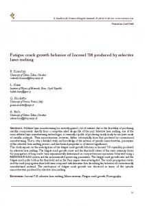
Schematical representation of the PSBs, which reach the surface and form intrusions and extrusions. . . . . . . . . . . . . . . . . . . . . . 2.2 Typical cyclic stress strain curve compared to monotonic curve. The two curves do not often coincide due to the strain softening/hardening effects in the early cycles. . . . . . . . . . . . . . . . . . . . . . . . . 2.3 The total strain amplitude versus life curve, obtained by the superposition of the linear elastic and plastic strain amplitude. In the low cycle fatigue (LCF) the behavior is generally described by the CoffinManson law, while in the high cycle fatigue (HCF) the Basquin law is employed. . . . . . . . . . . . . . . . . . . . . . . . . . . . . . . . . 2.4 The three mode of applying a load to a crack. . . . . . . . . . . . . . 2.5 Equivalent stress distribution proposed by the Irwin model. . . . . . . 2.6 Arbitrary contour around the crack tip to calculate the J integral. . . 2.7 A definition of the crack tip opening displacement δCT OD parameter. . 2.8 Typical log-log fatigue crack growth plot in metals. . . . . . . . . . . 2.9 Explanation of the plasticity induced crack closure effect. . . . . . . . 2.10 Schematic representation of the crack growth behavior as a function of the crack length. The solid line delimits the region between nonpropagating and propagating cracks [81]. . . . . . . . . . . . . . . . . 3.1 3.2 3.3

3.4 3.5

3.6

Basic block diagram of a phase locked loop. . . . . . . . . . . . . . . Magnitude Bode plot of the 2nd order phase locked loop. . . . . . . . Schematic diagram of the experimental setup for the fatigue crack growth (above). Detail of the microbeam mounted on the piezo stack and of the positioning system for the laser optics (below). . . . . . . . Functional schema of the employed circuit in the lock-in amplifier. . . Simulation (solid line) and experimental (dotted line) output of the PI controller subjected to a periodic square signal with a frequency of 250 Hz. . . . . . . . . . . . . . . . . . . . . . . . . . . . . . . . . . Simulation (solid line) and experimental (dotted line) output of the VCO subjected to a periodic square signal with a frequency of 40 Hz.

xxv

8

9

9 11 12 13 14 15 16

17 21 22

25 26

28 28

List of Figures 3.7

3.8

3.9

3.10 3.11 3.12 3.13 3.14 3.15 3.16 3.17

3.18 3.19 3.20

4.1 4.2 4.3 4.4

Simulation (solid line) and experimental (dotted line) output of the lock-in amplifier subjected to a periodic square signal after a frequency step of 5 Hz. . . . . . . . . . . . . . . . . . . . . . . . . . . . Reference spur effect: normalized FFT spectrum of the phase locked loop output when a pure sinus at 300 Hz is given at the input. The asterisks are the value calculated by the eq. 3.18. . . . . . . . . . . . Comparison of the models with the experimental measures: stable working region in Kp , Ki space of the PLL considering the effect of the lock-in internal PLL (iPLL) and of the resonator (Q=312 and ωr = 1551.505). . . . . . . . . . . . . . . . . . . . . . . . . . . . . . . Nyquist plot showing the definition of the gain and the phase margins. Phase margin as a function of Kp and Ki . . . . . . . . . . . . . . . . Simulated error signal upd after a phase step of π/4, including the effect of resonator Q-factor. . . . . . . . . . . . . . . . . . . . . . . . Simulated error signal upd after a frequency step of 5 Hz, including the effect of resonator Q-factor. . . . . . . . . . . . . . . . . . . . . . Simulated error signal upd after a frequency ramp of 5 Hz/s, including the effect of resonator Q-factor. . . . . . . . . . . . . . . . . . . . . . Measured error signal upd after a frequency step of π/2 with and without the resonator (Kp =0.3 and Ki =6). . . . . . . . . . . . . . . . Block diagram of the new setup containing a digital PLL circuit. . . . Waveform output signal upd (t) of a PFD generated by the given generic u1 (t), u2 (t) signals. On the right, schematic working principle of the phase frequency detector. . . . . . . . . . . . . . . . . . . Actual phase shift in a digital and analog PLL in function of the input signal amplitude. . . . . . . . . . . . . . . . . . . . . . . . . . . . . . Frequency stability as a function of the signal to noise level in the input signal (PLL without the resonator). . . . . . . . . . . . . . . . Phase shift between excitation and resonator motion as a function of time for both analog and digital PLL (Q=321 and fr =243 Hz). . . . Schematic representation of the sample design. . . . . . . . . . . . . The principal steps of the LIGA process. . . . . . . . . . . . . . . . Secondary electron SEM images: (a) overview of the Ni120 beam ; (b) detail of the sidewall and top surface (not polished). . . . . . . . Top, side and bottom images of a U notched Ni120 sample measured by LSM 5. The brightness is a relative measure of the height. A plot containing the raw data measured on a line is superimposed onto the images. . . . . . . . . . . . . . . . . . . . . . . . . . . . . . . . . . .

xxvi

28

30

35 36 38 40 40 40 41 42

43 45 46 47

. 50 . 52 . 57

. 58

List of Figures Cross section microstructure of a 30x30 µm2 beam, which has been polished by ion milling. The contrast is generated by ion channeling in a dual beam (SEM/FIB) microscope at EMPA, D¨ ubendorf. . . . 4.6 Tensile test setup: 1 translation stage, 2 load cell (max 50N), 3 objective of CCD camera, 4 sample. . . . . . . . . . . . . . . . . . . . 4.7 Results of 5 tensile tests on Ni120 as-plated samples plotted in an engineering stress-strain diagram. Effect of a heat treatment for 1 hour at 600◦ C on the tensile curve. . . . . . . . . . . . . . . . . . . 4.8 Modal analysis of the first three modes of a Ni120 sample by finite elements (Ansys). . . . . . . . . . . . . . . . . . . . . . . . . . . . . 4.9 FFT of displacement measured in the in-plane (blue) and out of plane (red) direction of the amplitude. The modal forms are also included showing the out of plane component of the displacement. . . . . . . 4.10 a) Compliance method for measuring R curve: the compliance is measured during the unloading in the force-displacement diagram. b) SENT specimen during the test. . . . . . . . . . . . . . . . . . . 4.11 Results of the compliance measurements on 4 specimens: a) Compliance measured during successive unloading. b) Plastic deformation measured as the displacement intercept of the fitting line during unloading. . . . . . . . . . . . . . . . . . . . . . . . . . . . . . . . . . 4.12 SEM image of the fracture surface after the toughness test. . . . . . 4.5

5.1 5.2

5.3 5.4

5.5 5.6

5.7

. 60 . 61

. 62 . 64

. 64

. 66

. 67 . 68

Meshing of the crack tip : degeneration of the brick elements to a wedge and the “spider web” mesh. . . . . . . . . . . . . . . . . . . . Distribution of the ∆K over the normalized thickness of an aluminum beam (10x10x400 mm3 ) excited in the first bending mode for different meshing divisions. . . . . . . . . . . . . . . . . . . . . . . . . . . . . . Typical mesh of the beam with a crack in the center. . . . . . . . . . Frequency and stress intensity factor convergence test as a function of the mesh refinement, calculated for an aluminum beam (10x10x400 mm2 ) excited in the first bending mode with a normalized crack length a/wb = 0.5 and a free end displacement of 1 mm. . . . . . . . . (a) Schematic model of the crack closure effect. (b) Effect of the crack closure on the measured frequency and amplitude. . . . . . . . . . . . Homogeneous solution of eq. 5.2: solid line represents the part of solution fulfilling the differential equation, while the dotted line does not. . . . . . . . . . . . . . . . . . . . . . . . . . . . . . . . . . . . . Non-dimensional plot relating the frequency drop with the crack length and the stress intensity factor. The points are the results of the finite element calculation, while the solid lines are the results of the analytical model [104]. . . . . . . . . . . . . . . . . . . . . . . . . . .

xxvii

70

71 72

73 74

75

76

List of Figures 5.8

Resolution plot as a function of the normalized crack length calculated assuming the typical values σf /f0 = 10−6 , σx /xmeas = 10−4 and xmeas = 10−4 . . . . . . . . . . . . . . . . . . . . . . . . . . . . . . . . 79

5.9

The crack growth on the Ni120 specimens employed for the accuracy measurement. a) Piezo stack displacement amplitude as a function of time. b) Resonator frequency and amplitude during the test. . . . 80

5.10 Calibration curve: crack length measured by SEM and crack length calculated from resonance test by pure elastic model and also including the elastoplastic correction. . . . . . . . . . . . . . . . . . . . . . 81 5.11 Frequency response curves of a Ni120 sample at different specimen amplitudes measured by means of PLL control system. . . . . . . . . 82 5.12 Frequency response curves of a Ni120 sample. Solid line is measured by phase control (closed loop), while points are response to a pure sine excitation (open loop). The sweep was performed with increasing frequency (fw) and decreasing frequency (rw). . . . . . . . . . . . . . 83 5.13 Frequency response diagram of a Ni120 sample measured with two different base excitation amplitudes y0 in open loop mode. . . . . . . 84 5.14 Schematic representation of the cantilever beam. . . . . . . . . . . . . 85 5.15 Infinitesimal small element of the beam before and after the deformation. The inextensibility condition is obtained imposing λ = 1. . . . . 87 5.16 Frequency response for a base excitation y0 = 125nm and y0 = 250nm obtained numerically from eq. 5.42 . . . . . . . . . . . . . . . . . . . 90 5.17 Restoring force plot of a Ni120 sample measured at its first in plane bending resonance frequency without the PLL control. . . . . . . . . 92 5.18 a) Section of the restoring force plot at x˙ = 0, which represents the stiffness. b) Section of the restoring force plot at x = 0, which corresponds to the damping force. . . . . . . . . . . . . . . . . . . . . 92 5.19 Normalized frequency response for 3 NiFe and 3 Cu sample. . . . . . 93 5.20 Effect of the cyclic loading on the frequency response curve of a Ni120 sample. . . . . . . . . . . . . . . . . . . . . . . . . . . . . . . . . . . . 94 5.21 a)Illustrative plot of the nonlinear hysteretic contribution in the constitutive equation. b)Measured frequency response plot of a Ni30 sample (blue circles) and the fitted plot (red crosses) obtained with the following parameters: f0 = 238.868, ζr = 1.113 ∗ 10−4 , δh = 7.365 ∗ 108 , χh = 0.6447. . . . . . . . . . . . . . . . . . . . . . . . . . 96

xxviii

List of Figures 6.1

6.2

6.3 6.4

6.5 6.6

6.7

6.8

6.9

a) Finite element simulation of a Ni120 sample at its second resonance mode representing the von Mises stress. The highest value of the stress is located near the fillet by the clamped plate. b) Stress-life diagram for the unnotched Ni120 and Ni60 samples. The trend line for both sample types (solid line) is compared to the bulk nickel values, obtained for cold drawn and annealed specimen [31]. LIGA nickel samples have a fatigue resistance comparable to bulk cold drawn nickel.100 Frequency evolution during the stress-life test for two samples at different loading: the sample loaded at 460 MPa represents the typical behavior in the finite life region, while the sample at 350 MPa represents the typical behavior slightly under the endurance limit σe . . . . 102 Fatigue crack growth test on 3 V-notch Ni120 specimens with the same ∆K-increasing method without pre-cracking. . . . . . . . . . . 103 Effect of the normalized ∆K-gradient C in the load shedding procedure. A curve obtained with the ∆K-increasing method is added as a comparison. . . . . . . . . . . . . . . . . . . . . . . . . . . . . . . . 105 Fatigue crack growth on the specimens with width 120, 60 and 30 µm.107 Fatigue crack growth in the Ni120, Ni60 and Ni30 samples. The amount of data was reduced by polynomial fitting. As a comparison, the values published by Yang [129] on a 10 mm CT sample are also reproduced in this plot. . . . . . . . . . . . . . . . . . . . . . . . . . . 108 a)Crack nucleation from the notch root in a Ni120 sample (bottom view). b)Crack arrest due to a path deflection in another Ni120 sample (top viev). . . . . . . . . . . . . . . . . . . . . . . . . . . . . . . . 110 a)Fracture surface of a Ni120 sample after being tested in a fatigue crack growth experiment. b)Detail of the fracture surface at higher magnification. . . . . . . . . . . . . . . . . . . . . . . . . . . . . . . . 111 Fracture surface after fatigue crack growth test in a Ni60 (a) and Ni30 (b) sample. . . . . . . . . . . . . . . . . . . . . . . . . . . . . . . . . 112

A.1 Frequency response of the piezostack measured at the steady state with lock-in amplifier (excitation 3V, with and without servo control). 120 A.2 Static calibration curve given by the manufacturer with and without servo control. . . . . . . . . . . . . . . . . . . . . . . . . . . . . . . . 120

xxix

List of Figures

xxx

List of Tables 3.1

Parameters used for the simulation . . . . . . . . . . . . . . . . . . . 27

4.1 4.2 4.3 4.4

Sample principal sizes (µm). . . . . . . . . . . . . . . . . . . . . . . . Sulfamate nickel bath composition. . . . . . . . . . . . . . . . . . . . Solutions tested for etching the copper sacrificial layer. . . . . . . . . Surface roughness parameters of beams. Ra and Rq were computed for a curve filtered according to DIN4776, while Rt was determined for the unfiltered curve. . . . . . . . . . . . . . . . . . . . . . . . . . . Averaged tensile results of the 5 Ni120 as-plated samples and of the annealed sample. . . . . . . . . . . . . . . . . . . . . . . . . . . . . . Tensile results of other groups, taken from the literature. . . . . . . . Results of the measured trial toughness values KQ of 4 Ni120 samples. Results of the toughness measurements on microsamples in other groups. . . . . . . . . . . . . . . . . . . . . . . . . . . . . . . . . . . .

4.5 4.6 4.7 4.8 6.1

6.2

50 54 56

59 61 62 66 67

Experimental results measured in the present work [*] and values found in the literature for the stress-life of nickel LIGA microsamples. The ≈ symbol means that the corresponding value was extracted from the Wöhler diagram. In the testing method the symbol B means Bending, while T means Tensile. . . . . . . . . . . . . . . . . . . . . . 101 Parameters of the Paris law obtained by fitting the curves in fig. 6.4 as a function of the normalized ∆K-gradient. . . . . . . . . . . . . . 106

xxxi

List of Tables

xxxii

Chapter 1 Introduction The past decade saw a clear trend towards the miniaturization of devices in different application fields, amongst which the electronic industry is probably the best example. This new emerging discipline has been broadly speaking referred to as micro-nano technology. The enormous interest in this area is justified by the unexplored possibilities of new applications and by the new facilities, which enable to study materials at an intermediate scale between the atomistic view and the conventional macroscopic dimensions. In such a wide and still active field of research, this thesis has focused its interest on materials for micro electro mechanical systems. These devices have found many diverse applications in fields such as inertial guidance and control, fluid sensing, acoustics, optics, robotics and biomechanics. A high level of knowledge in several engineering disciplines is needed in order to successfully fabricate these microdevices. Therefore structural reliability receives generally less attention than the development of the fabrication process. On the other hand, the reliability of these components is a key factor for their future commercialization. Moreover, the different technologies involved in the device fabrication and the small dimensions can have unforeseen effects on the material behavior. A typical example is the so-called “size effect”, which deals with the deviation of the intrinsic material properties as the specimen approaches a characteristic length scale [9]. Therefore new methods, facing the problems of handling small specimens and measuring tiny forces, have to be developed in order to measure and to understand the material properties at the microscopic scale. The final step will be to provide the engineers with standardized tools to measure the material parameters necessary to simulate the microsystems’ behavior and design them.

1

1.1. MEMS reliability: previous research

1.1

MEMS reliability: previous research

The small dimensions of most MEMS devices have posed several issues in the fabrication and in the service life of such components. The most common failure mechanisms encountered in the literature are due to either a static overload, which leads to fracture, or to a large amount of cycles, which induces a fatigue damage. Other failure modes have also arisen, such as creep deformation, wear damaging or some other mechanisms peculiar to the microsystems such as stiction, delamination, dielectric breakdown and electromigration [125]. Many research groups have spent a considerable effort in developing testing methods to study each of these mechanisms and to enrich the common knowledge, as a first step towards the engineering of MEMS devices. Most of the work done on the characterization of specimens at the microscale is concentrated on the determination of the elastic modulus and the strength by means of static tests. The main approach is to scale down the tensile setup, which is the best method to obtain in a straightforward manner the stress-strain curve, but new solutions have been developed to overcome the major issues, i.e. the specimen handling and the measurement of the strain [108]. Other methods such as bulging test, nanoindentation, microbeam bending and torsion have been used by many authors as alternative methods. The advantages and the disadvantages of each methods and the common sources of errors have been reviewed in [63] and [114]. An overview of the tensile data measured by many authors for metallic microsamples is presented in [26], where it is observed that the mechanical properties for the same material can vary widely and that a more systematic work is still needed to understand the influence of the material microstructure at small scales. The study of a dynamic process like fatigue poses new requirements on the equipment, which classical setups cannot fulfill: in fatigue crack growth testing very small cracks have to be measured and the measurement procedure should be reliable and possibly automatic. Moreover, the system should be able to monitor or to control the force and the displacement in real time and the loading frequency should be enough to provide a reasonable time of testing. In the following pages the methods and major achievements of previous groups regarding fatigue testing are listed. In particular, some of them have focused their attention on the study of the fatigue micromechanism in micron-sized specimen. Boyce [17] at Sandia National Laboratories examined the high cycle fatigue in LIGA nickel beams from the material point of view. He reported the degradation introduced by the cyclic deformation in the microstructure analyzed by means of a Electron BackScatter Diffraction (EBSD) technique and he highlighted the important role played in the crack initiation by the oxidation film together with the motion of the persistent slip bands.

2

Chapter 1. Introduction

Kraft et al. [62, 131] proposed two techniques for fatigue testing: microtensile polyimide samples with thin Copper sputtered layer and a microbending SiO2 beam covered by an Ag thin film and actuated by a nanoindenter. They observed the roughening of the surface in a FIB and they explained by means of dislocation theory that the formation of the extrusions is controlled by the grain size and the film thickness. In an other work [38], they described the process of the voids and extrusions formation on the 100nm thick Al metalizations in a Surface Acoustic Wave (SAW) filter at ultrahigh frequency (GHz). Soboyejo et al. [4] performed stress-life experiments on LIGA nickel beams with thickness of 70 and 270 µm and found an increase in the fatigue resistance on the thinner specimens. They enlarged the analysis to low cycle fatigue [72] and they explained the length scale effect by a dislocation strain gradient plasticity theory. In some recent publications [129, 130], they observed and described the growth method of a crack by means of SEM and FIB images, documenting for the first time the anomalous behavior of the short crack in MEMS. Other studies on the fatigue crack growth in small probes are relatively rare and generally restricted to through-thickness cracks in foils and films. Two of this works, written by Alic and Asimow [3, 2], are dated back to almost 40 years ago and they dealt with the qualitative description of the crack propagation in copper, brass and tantalum thin foils. In a relatively recent publication [51] Hadrboletz et al. performed fatigue crack growth analysis on wrought and electroplated copper, aluminum and molybdenum foils with a thickness between 25 and 250 µm. Testing was performed gluing the sample over a slot fabricated on an aluminum bar. The bar was excited in longitudinal resonance, the deformation recorded with a strain gage and the crack monitored by a traveling microscope. Just on wrought copper foils, they observed an irregular crack growth typical of short cracks and associable with the grain boundary interactions, although the crack was not physically short. Moreover they related the increase of the threshold ∆Kth with the relative increase of the ratio of foil thickness to grain size. As far as the technique is concerned, the following studies have been performed. The pioneering work of Connally and Brown [25], who developed the first phase controlled resonating microdevice based on an electrostatically actuated beam with a tip mass to evaluate the fatigue of single crystal silicon, shows qualitatively that the frequency change can be related to the compliance change introduced by a crack.

3

1.2. Scope and outline of the present work They reported that a small crack growth region, which was independent of the stress intensity factor, was present before the final failure. This work had several followers, who have tried to explain why silicon at the microscale has a fatigue-like behavior, while bulk silicon is not susceptible to fatigue. Many experimental data and some suggested micromechanisms have been collected and compared in [6]. Schlums and Dual [103, 104] developed a compliance method to evaluate quantitatively the fatigue crack growth curves of metallic macrobeams excited in a bending resonance mode. They pointed out the importance to correct the frequency and the amplitude of the resonator for accounting the nonlinear dynamical effect generated by the crack surfaces contact. Moreover, they show that the technique could be applied to microspecimens [102], but they did not further analyze the experimental results.

1.2

Scope and outline of the present work

Although some work on fatigue and crack growth in metallic microspecimens has already been published, there is still a lack of knowledge on the topic and the data available is insufficient. The modeling of the fatigue mechanism is a complex subject especially at the microscale, where few experimental data is available due to the difficulties to perform crack growth studies. This work investigates the capability of the technique proposed by Schlums and others to measure the crack growth in micron-sized specimens using a phase controlled resonating system. One of the advantages of this method is that the crack size is measured as a fraction of the sample size and therefore there is in principle an enhanced crack resolution in small probes, as compared to traveling microscope for example. Therefore, it is interesting to determine the resolution and the accuracy of this technique and to study the factors that could influence these quantities. The application of this technique to the microspecimens opens the possibility to characterize in a simple way the crack growth rate at the microscale. This approach intrinsically assumes that the crack growth can be predicted by means of the fracture mechanical tools. This aspect is actually not obvious and therefore the implications of this approach are discussed. Moreover, the small dimensions of these specimens make the presence of the crack tip plasticity not negligible and the application of the linear elastic theory questionable. It is not clear if a material size effect could appear when the scale of the sample is reduced or if in micron-sized specimens the plasticity induced crack closure effect and the short crack behavior are present in a similar way to macrosamples. Before being able to answer these questions, some work to improve the understanding of the setup, to prepare and characterize the samples and to model their

4

Chapter 1. Introduction dynamical behavior is necessary. The structure of the present study is organized in the following chapters. The fundamental concepts of fatigue and fracture mechanics are briefly reviewed in chapter 2. A model to study the dynamic behavior of the measuring system and a method to determine the key parameters based on stability and performance considerations are presented in chapter 3. Some enhancements of the first setup version are proposed and built into a unique customized instrument. In chapter 4, the optimization of the samples’ fabrication process is described, which is a necessary step for the production of good quality specimens. Moreover, their tensile properties, their toughness, the material microstructure, their effective dimensions and their surface roughness are precious data, which gives a complete overview of the sample characteristics and enables a systematic comparison with the results of other groups. A method to calculate the mechanical model of the resonator by means of finite elements is explained in chapter 5. The method enlarges the application of the phase controlled resonating fatigue testing (PCRFT) also to complex geometries. Moreover, a one-dimensional nonlinear analytic correction, which describes the effects of the wedging phenomenon during the crack closure on the frequency and the amplitude, is developed to explain the experimental results. In this chapter the source of the nonlinear effects, which have been observed in a closer analysis of the frequency response curves in the unnotched samples is further investigated. Nonlinearities can produce frequency-amplitude dependence and affect the dynamic behavior of the sample during the experiments. Chapter 6 presents the results of the stress-life experiments and the fatigue crack growth tests on the nickel microbeams. The influence of the testing condition and the effect of the beam width on the fatigue crack growth outcomes have been considered. From the analysis of the fracture surface more information about the fatigue micromechanism has been gained to support the obtained results.

5

1.2. Scope and outline of the present work

6

Chapter 2 Basic concepts of fatigue and fracture mechanics T

his chapter introduces the reader to the main approaches to study the fatigue phenomenon: high cycle fatigue and fatigue crack growth. Moreover, a review of the fundamental concepts of fracture mechanics in fatigue crack growth is provided.

2.1

Fatigue

Fatigue is a well-known physical phenomenon that affects the materials subjected to cyclical loading conditions. Although the first work on fatigue are dated back to the first half of the nineteenth century and many useful observations have been made in the past century, thanks also to the invention of the electron microscopes, a complete understanding of the process and an accurate enough design method to fulfill the challenging requests of the market are still missing. The brief introduction to fatigue and fracture mechanics presented in this thesis is based on the following reference books: the fatigue from the microstructural point of view is described by Suresh [118] and the mechanical approaches to its study by Radaj [93]. The basic and advanced concepts of fracture mechanics are taken from Anderson [7] and Saxena’s books [98], while the microstructural aspects in the fatigue crack growth process can be found in Krupp’s book [64]. Historically the fatigue failure process is divided in crack initiation and crack propagation. This division is not well defined and the limit between the two stages has been reduced over the years, due to the improvement in the understanding and modeling of the crack advance in the early stages. However, it is well established that in metals the origin of the fatigue cracks are related with the slip of the material lattice due to the dislocation motion. Studies on fcc single crystal metals [118] have revealed that the plastic deformation is mostly localized along the so-called persis-

7

2.1. Fatigue intrusion

extrusion

bulk PSBs

Figure 2.1: Schematical representation of the PSBs, which reach the surface and form intrusions and extrusions. tent slip bands (PSB) and these are the precursors of crack formation. The exact micro mechanism of crack initiation depends on the metal: in high purity metals the PSBs reach the free surface producing intrusions and extrusions (see fig. 2.1), which act as local stress raisers promoting the crack formation. In commercial alloys, however, other heterogeneities such as inclusions and pores are frequently the preferred crack initiation sites. Once the crack has nucleated, it undergoes first a short crack growth phase and then propagates as a long crack under the control of the deformation field at its tip till the final fracture. When plotting the stress strain curve of metals subjected to cyclic loading (see fig. 2.2), a typical hysteresis loop is obtained after a transient phase of about a few hundred cycles. The curve that connects all the vertices of the hysteresis loops at different loading amplitude is called cyclic stress strain (CSS) curve and it can differ slightly from the conventional monotonic tensile curve. The example represents a strain softening behavior, but, depending on the material conditions, it is possible to have also a strain hardening behavior. For some alloys the steady state hysteresis loop is never achieved and therefore a meaningful CSS curve cannot be defined. In the traditional approach, the fatigue property consists in an experimental plot, which relates the amplitude of loading to the number of cycles to failure of a standardized specimen, without differentiating between crack initiation and propagation. This phenomenological curve, sketched in fig. 2.3, is mathematically described by the Basquin law in case of stress controlled tests, which is typical for high cycle fatigue (HCF), and by the Coffin-Manson law for the strain controlled low cycle fatigue (LCF). In both cases the traditional approach does not account for the presence of a preexisting crack and the loading parameters are calculated on the nominal specimen section. In the fracture mechanics approach the crack length in a standard pre-cracked specimen is measured as a function of the cycles and its growth rate is mathematically related to the proper fracture mechanics parameters. Although still phenomenological, the fracture mechanics philosophy has contributed to a better understanding of the fatigue damaging process and its concept is generally applied in the most challenging fields, as for example in the aerospatial industry.

8

Chapter 2. Basic concepts of fatigue and fracture mechanics

σ monotonic loading

hysteresis loop

CSS

ε

Figure 2.2: Typical cyclic stress strain curve compared to monotonic curve. The two curves do not often coincide due to the strain softening/hardening effects in the early cycles.

Log total strain

LCF

HCF

∆εp 2 Coffin-Manson

Basquin ∆εe =∆σ 2 2E Log cycles to failure

Figure 2.3: The total strain amplitude versus life curve, obtained by the superposition of the linear elastic and plastic strain amplitude. In the low cycle fatigue (LCF) the behavior is generally described by the Coffin-Manson law, while in the high cycle fatigue (HCF) the Basquin law is employed.

9

2.2. Fracture mechanics

2.2

Fracture mechanics

Fracture mechanics is concerned with the structural integrity of structural components containing sharp defects, namely the cracks. Conventional local stress and strain criteria are generally not able to predict the conditions for the crack to advance and the number of cycles needed before the complete failure. The reason is due to the fact that under small strain condition a stress and strain singularity at the crack tip is present and therefore conventional local failure criteria are not applicable. The key idea in fracture mechanics is the concept of similitude, which implies that the crack tip condition can be uniquely described by a limited set of loading parameters. In case of a stationary crack, two different components made of the same material are going to fail at the same loading local parameter value (for example the K or J, where K is the stress intensity factor and J the J-integral.). The main peculiarity in the fracture mechanics approach is then that the behavior of the crack is controlled by the stress and strain distribution of a region ahead of the crack tip. It must be remembered that fracture mechanics is not a competing theory to the usual strength approach, but it completes the mathematical description of the possible failure modes. Under some circumstances, a cracked component can fail by plastic collapse rather than crack growth.

2.2.1

Linear elastic fracture mechanics (LEFM)

Westergaard and Irwin [7] were among the first researchers, who calculated and published the analytical solutions of simple cracked configurations under the assumptions of a linear elastic and isotropic material. In a general case, the stress field can be expressed in the form of eq. 2.1, where r and θ are the polar coordinates with origin at the crack tip. ∞ X K (m) Am rm/2 gij (θ) fij (θ) + σij (r, θ) = √ 2πr m=0

(2.1)

Regardless of the configurations, the solution presents a term, which varies with √ 1/ r and dominates the stress distribution near the crack tip. The proportionality factor K is the stress intensity factor, which represents the magnitude of the loading in proximity of the crack tip. There are three modes, in which a crack can be loaded and they are sketched in fig. 2.4. They result in three independent stress intensity factors KI , KII and KIII , which are not directly comparable, although they have the same dimensions (namely MPa m1/2 ), because the functions fij and gij are different for the three modes. Solutions for the stress intensity factors can be calculated analytically just in a few cases, therefore handbooks are available reporting the

10


Mode I

Mode II

Mode III

Figure 2.4: The three mode of applying a load to a crack. solutions obtained by numerical methods for many configurations written in the general form: √ K = σ ∞ Y (a) πa (2.2) where σ ∞ is the reference remote stress, Y (a) is a geometrical factor and a the crack length. When K is greater than the critical condition Kc (a material parameter), the crack grows. The energy release rate G (eq. 2.3), as proposed by Irwin [7], is a parameter equivalent to the stress intensity factor, but it is based on energetic considerations. G=−

dΠ dAc

(2.3)

The total energy Π = V − Fw is the elastic stored energy V minus the work Fw done by the external forces and Ac is the surface of the crack. Following the idea of Griffith, Irwin individuates the critical condition Gc when the energy released by the crack growth is equal to the energy necessary to form two new crack surfaces. Gc and Kc are considered material properties, which can be determined experimentally on cracked standard samples and they quantify its toughness. The relation, which connects the global parameter G and the local parameter K, is G=

K2 E0

(2.4)

where E 0 = E for plane stress and E 0 = E/(1 − ν 2 ) for plane strain. Only a few materials have a purely linear elastic behavior. Therefore it is appropriate the question if the linear elastic fracture mechanics is still applicable to all other materials. Moreover, the predicted infinite stress at the crack tip is in real

11


σyy

θ=0 elastic

σY rY

elastoplastic

r

rp

Figure 2.5: Equivalent stress distribution proposed by the Irwin model. materials not possible, because inelastic deformations such as plasticity in metals and crazing in polymers take place thereby increasing the crack tip radius. The stress analysis becomes progressively inaccurate as the size of this inelastic region grows as compared to the dimensions of the specimen. As long as the inelastic region is ”small”, LEFM is still applicable with some simple correction models, otherwise the elastoplastic fracture mechanics approach should be used. The first approach to extend LEFM to materials with an elastic purely plastic behavior was proposed by Irwin [98]. The model considers just the normal stress σyy in the crack plane (see fig. 2.5). In the elastoplastic case, a plastic region with a size of rp is formed near the crack tip, while outside of this region the material remains in elastic conditions and the stress decreases moving away from the crack tip. In order to find the equivalent elastic distribution, which describes the stress field outside the plastic zone, Irwin proposes that the forces resulting from the integration of the elastic and of the elastoplastic stress distributions are equal. The condition is equivalent to imposing the equality of the two highlighted areas in fig. 2.5. It results in the definition of an effective stress intensity factor Kef f , calculated assuming that the crack length is extended by a plastic radius rY (see eq.2.5). 1 K I 2 rY = zπ σY

z=

2 6

plane stress plane strain

(2.5)

Another well-known correction is the strip yield model proposed by Dugdale [98], which, although based on slightly different assumptions, produces a correction approximately in agreement with the Irwin model up to σ ∞ /σY = 0.85 [7]. According to the ASTM E399 standard, the size requirement (Small Scale Yielding condition) of the sample expressed in eq. 2.6 must be met for the correct appli-

12

Chapter 2. Basic concepts of fatigue and fracture mechanics cability of LEFM. a, ts , (wb − a) ≥ 2.5

KI 2 = 2.5zπrY σY

(2.6)

The condition, which is based on experimental observations, imposed that the crack length a, the thickness ts and the ligament (wb − a) are larger than roughly 50 rY to ensure a size independent value of the toughness KIC . The requirement on the thickness ensures just that the crack grows under plane strain condition, which shows in general the lowest critical value. The application of the plasticity corrections can extend further the validity of LEFM, but it must be remembered that these approximations are still based on the linear elastic theory. On the other hand, ASTM E399 conditions are very stringent and it is often very difficult to measure a valid KIC for a structural material [7].

2.2.2

Elastoplastic fracture mechanics (EPFM)

The J contour integral, proposed by Rice, can be viewed as the extension of the concept of the energy release rate G to nonlinear material behavior. Strictly speaking, the J-integral is applicable just to nonlinear elastic material behavior, but it can be adopted also for elastoplastic materials as long as no unloading occurs, because just under this condition the stress-strain curve of both materials coincides. Similar to G, J is defined as dΠ (2.7) J =− dAc where Π is the total energy and Ac the crack area. The total energy Π = V − Fw is equal to the stored energy V minus the work done by the external force Fw . However, unlike G, J represents rather the absorbed than the released strain energy, because when the crack grows in elastoplastic materials, not all the deformation energy in the unloaded region will be recovered.

y

x Γ

ds T

Figure 2.6: Arbitrary contour around the crack tip to calculate the J integral.

13

2.2. Fracture mechanics One property of J is that it can be calculated as the following path independent line integral (see fig. 2.6) Z εij Z ∂ui ds) we = σij dεij (2.8) J = (we dy − Ti ∂x 0 Γ where we is the strain energy density, Ti are the components of the traction vector normal to ds and ui the components of the displacement. If the material law can be described by the Ramberg-Osgood equation (eq. 2.9), Hutchinson, Rice and Rosenberg [98] showed that J, similarly to K, can describe the stress distribution at the crack tip and it can be adopted as stress intensity parameter. σ σ m ε = +α (2.9) ε0 σ0 σ0 As in the linear elastic case, the stress distribution (eq. 2.10) contains a singularity for r = 0, because this model does not take into account the crack tip blunting, which is produced by the large finite strain. 1 EJ m+1 σij (r, θ) = σ ˜ij (m, θ) (2.10) ασ02 Im r Im is an integration constant depending on the strain hardening exponent m and σ ˜ij is a dimensionless function. In a similar way as in LEFM, it can be stated that the J is able to characterize the toughness of a material as long as the finite strain zone at the crack tip remains small in comparison to the in-plane dimensions of the sample. δ CTOD

Figure 2.7: A definition of the crack tip opening displacement δCT OD parameter. Another well-known parameter, which characterizes the toughness in the elastoplastic regime is the crack tip opening displacement (CTOD). Its definition is explained in fig. 2.7: The dashed line is the crack before loading and the solid line after loading. δCT OD represents a measure of the crack tip blunting. Its value can be correlated to J by eq. 2.11 as explained in [100], J = βm σY δCT OD where βm is a non-dimensional factor and σY is the yielding stress.

14

(2.11)


2.2.3

Fatigue crack growth

The possibility to employ fracture mechanics concepts to describe the crack growth due to fatigue was demonstrated by Paris in the early 1960s. Although in that time the proposal aroused many discussions, nowadays it is the basis of the well-known damage tolerant approach for the fatigue design. Plotting in a log-log diagram the crack growth rate da/dN as a function of the stress intensity ratio difference ∆K = Kmax −Kmin , Paris found a curve similar to that in fig. 2.8. The curve can be divided in three regions: the region I corresponds to the threshold, where the crack propagation rate approaches zero as ∆K reaches the threshold ∆Kth . At higher ∆K levels, in region III, the crack accelerates as the Kmax approaches the static fracture toughness of the material. In the region II, the curve appears linear and it da dN

Region I

Region II

∆Kth

∆K

Region III

∆Kc

Figure 2.8: Typical log-log fatigue crack growth plot in metals. can be mathematically described by a power law like eq. 2.12, which was originally proposed by Paris and Erdogan [64]. da = B∆K n dN

(2.12)

In the following years many empirical equations have been proposed, which tried to completely describe the sigmoidal form and to include the effect of the mean stress through the stress ratio R, but the Paris law remains the most well-known. The stress ratio is defined as ∞ σmin (2.13) R= ∞ σmax ∞ ∞ where σmax and σmin are the maximal and minimal values of the reference stress. B, n are considered to be material properties, although several times the incomplete self-similarity of the Paris law has been highlighted [91, 96]. In other words, based

15


plastic wake

Kmax

crack tip plasticity

Kcl Kmin t

Figure 2.9: Explanation of the plasticity induced crack closure effect. on dimensional and similarity considerations it can be demonstrated that the coefficients B, n must depend on the size of the specimen. These observations have not found a clear answer yet, but Paris law is still a widely accepted tool for lifetime predictions. The threshold ∆Kth can be viewed as well as a material property, if it is considered that this value is the sum of an intrinsic component and a component dependent on the stress ratio R. Most of the equations, which relate the threshold value to the stress ratio, invoke the crack closure effect as explanation. A review of these equations is given in [75]. The first observations about the crack closure effect are due to Elber [41]. He noticed that many cracked samples showed an anomaly in the compliance during the unloading phase. He believed that this effect was due to the premature contact between the crack surfaces and he postulated a reduction of the driving force through an effective stress intensity factor ∆Kef f = Kmax − Kcl . Suresh and Ritchie [119] proposed five different micromechanisms to explain the origins of the crack closure phenomenon. Probably the most well studied is the plasticity induced closure, which assumes that the crack tip plasticity leaves a plastic wake on the crack surfaces (see fig. 2.9), producing a wedge effect. During the last three decades the concept was further developed and employed also to explain with some success the history effects on the crack growth. Its application is still complicated by the fact that the level of closure is not a material parameter, but it depends mostly on the loading history. Therefore crack closure is a quantity which has to be experimentally determined and a consistent procedure has to be followed to avoid large errors. One observation, which was previously shortly mentioned, is that the crack growth is dependent on the loading history, while the measurement of the Paris curve assumes quasi steady state conditions. However the measurement of the crack growth curve is generally obtained by one sample test: the load is slowly changed to cover the desired stress intensity range and the corresponding crack growth rate is calculated by interpolation and differentiation of the crack length in function of the number of cycles. Particular attention has to be paid in avoiding artifacts coming by

16

Chapter 2. Basic concepts of fatigue and fracture mechanics a sudden load change. A clear example of the history dependence is the well-known retardation effect: a half cycle overload produces a transitory deceleration of the crack growth, till the crack overcomes the plastic zone produced by the overload. Many semi-empirical approaches have been proposed [112] to account for the history dependence, but an exhaustive model is not available due to the complexity of the topic. As a last peculiarity of fatigue crack growth, it is worth mentioning the anomalous high rate of growth, even below the threshold value, of cracks, whose size is “small”. A clear definition of what is a short crack does not exist and the subject is still subject of ongoing research. Following the categorization proposed by Suresh and Ritchie [118], there are three types of short cracks: • Microstructural short flaws, whose length is comparable to the dimension of the microstructure, like for example the grain size. • Mechanically short flaws, which are embedded in their near tip plastic region or they are engulfed by the plastic strain field of a notch. • Physical short flaws are nominally amenable of being described by LEFM, but they show an anomalous crack growth rate.

EPFM

Log stress range

σe MFM

LEFM da =0 dN non-propagating cracks Log crack length

Figure 2.10: Schematic representation of the crack growth behavior as a function of the crack length. The solid line delimits the region between non-propagating and propagating cracks [81]. The fact that cracks are able to propagate also below the threshold, but they eventually stop at a certain length, was explained by Miller [81] introducing the three distinct threshold regions. He described graphically as reported in fig. 2.10 the three regions of crack growth in full agreement with the definition of Suresh and Ritchie.

17

2.2. Fracture mechanics In the early stages, when the crack spans one or two grains, the crack growth can be modeled by the microstructural fracture mechanics (MFM), which accounts for material anisotropy and dislocation dynamic. As the crack grows further, the orientation of the grains and the interactions of the crack with the grain boundary become less important, but the crack is still too short for creating a K dominance region and therefore EPFM are preferred to describe the crack growth in this region. Once the crack is longer compared to its own crack tip plasticity, then LEFM is the suitable tool. Anomalies of the crack growth in the physical short crack region are explainable according to Newman [87] by the fact that the crack closure effect has not fully developed yet at this stage. On the contrary, he considers rather the long crack growth as an exception of the short crack behavior.

18

Chapter 3 Measuring principle and controller model T

his chapter describes the measurement principle of the resonating fatigue crack growth test. Details on the stability and the dynamic response of the feedback control system are reported, in particular the effects of the control parameters and the presence of a resonator are investigated. Moreover, a digital implementation of the control system has been proposed to improve system reliability.

3.1

Introduction

The frequency of a signal can be easily and cheaply measured with a very good accuracy in comparison to the amplitude. Two methods are in principle available to measure frequency: zero crossing detection and the Phase Locked Loop (PLL). Implementation, design and characteristics of both methods are treated and compared in [24]. The main advantage of a PLL is its ability to recover the information embedded in the frequency also from a very noisy input signal and, at the same time, to produce a phase shifted and “filtered” version of the input signal. A PLL is actually a circuit capable to produce an output signal synchronized with a reference input signal. Due to its low pass characteristic, a PLL reduces the phase noise of the input signal. Therefore, this device is widely in use in telecommunication for modulating/demodulating a signal or to distribute clock timing pulse in computers. For that reason many different implementations have been proposed in the last three decades [68]. Another particularly interesting application is when the PLL is employed to excite a mechanical resonator, whose resonant frequency is in general a function of the material property, boundary condition and geometry. In this case, the resonator is used as a transducer to measure the change of one aforementioned parameter, while

19

3.2. Linear theory the PLL is the device responsible to maintain the resonance condition, to filter and to interpret the signal before the read out. Applications of the PLL technique in this direction were largely exploited at the Institute of Mechanical Systems (ETH Zurich): measurement of the viscosity [37], characterization of soft biological tissues [122] and studies of gravitational interactions [126] have been performed by means of a PLL controlled system. Many other interesting applications have been found by several different authors in particular as electronic elements for MEMS resonators, where the main advantage is the possibility to produce a device, which integrates controlling electronics, read out and sensor. To cite just a few example, accelerometers, gyroscopes, chemical sensors and many others were successfully built [73, 44, 14]. For the proposed fatigue crack growth application, the establishment of a model for the feedback control system is of utmost importance, in order to understand and to interpret the experimental results. Then the effects of the choice of the control parameters and the mechanical resonator properties on the stability and the dynamic of the system are the main topics of interest. The first step is a brief review of the well established linear theory of a phase locked loop.

3.2

Linear theory

The basic structure of a PLL is represented in fig. 3.1, where the main functional blocks are: • A voltage controlled oscillator (VCO) • A phase detector (PD) • A loop filter (LF) The peculiarity of a phase locked loop in comparison with a standard feedback loop control system is that the input and output are phase signals as a function of time. The typical form of phase signal can be written as uin (t) = Uin cos(Ω0 t + θin (t))

uout (t) = Uout cos(Ω0 t + θout (t))

(3.1)

where the information is carried neither in the amplitudes Uin , Uout nor in the frequency Ω0 , but in the phases θin , θout . The behavior of such a servo system can be studied properly by working in the Laplace domain. In our experiment, the input signal θin (s) contains the information about the motion of the resonator and it is the signal that has to be tracked by the phase locked loop. This signal is fed into the phase detector together with the signal θout (s) coming from the voltage controlled oscillator. The phase detector in the locked state produces a signal, that is ideally just directly proportional to the phase shift between the two signals:

20

Chapter 3. Measuring principle and controller model uin(t)

Phase Detector upd(t)

uout(t)

Loop Filter

Voltage Controlled Oscillator

uf(t)

Figure 3.1: Basic block diagram of a phase locked loop. upd (s) = Kpd θe (s) = Kpd (θin (s) − θout (s)).

(3.2)

The PLL is considered in the locked state when the input and the output signal are synchronized, namely the phase error θe (s) is almost zero over a given time interval. The resulting signal upd (s), whose low frequency part represents the phase error between the input and output, are passed to the loop filter, which has the task to suppress the higher frequencies and to minimize the phase error. Many loop filter configurations are possible, but in this work just the PI filter has been considered, which has the advantage to have an unlimited hold range. In other words, due to the presence of the integrator in the filter, the PLL is theoretically able to maintain the locked state with any frequency of the input signal uin (s). The general expression for the transfer function of a PI filter followed by a low pass filter of the (n − 1)th order is: Ki uf (s) 1 = Kp + (3.3) Hf (s) = upd (s) s (1 + τ2 s)...(1 + τn s) where τ2 , ..., τn are the low pass filter time constants and Kp , Ki are the proportional and integral coefficients of the PI filter. The loop filter is actually the main responsible of the PLL behavior, because the parameters of the other blocks are generally fixed, while the filter parameters have to be designed. The voltage controlled oscillator is an electrical oscillator, whose frequency Ω(t) can be adjusted around its central value Ω0 by a modulation frequency ∆Ω(t), which is controlled by the external voltage signal uf (t). Ω(t) = Ω0 + ∆Ω(t) = Ω0 + Kvco uf (t)

(3.4)

Integrating the modulation frequency ∆Ω(t) in time and rewriting it in the Laplace domain leads to: Kvco θout (s) = (3.5) Hvco = uf (s) s Combining the eq.3.2, 3.3 and 3.5 it is possible to write the simplified linear model of a PLL (eq.3.6). θout (s) Kpd Kvco Hf (s) Hpll (s) = = (3.6) θin (s) s + Kpd Kvco Hf (s)

21

3.2. Linear theory 10

Hpll(iω)

(dB)

5 ζpll=5

0

3

-5

1 0.7 0.5 0.3

-10 -15 -20 -25 -1 10

0

10 ω/ωpll

10

1

Figure 3.2: Magnitude Bode plot of the 2nd order phase locked loop. Considering the simple case where the PI is a first order filter (τ2 = ... = τn = 0) and rewriting the equation in a normalized form 2 2ζpll ωpll s + ωpll Hpll (s) = 2 2 s + 2ζpll ωpll s + ωpll

ωpll =

p Kpd Kvco Ki

and

ζpll =

ωpll Kp 2Ki

(3.7)

(3.8)

where ωpll is the natural frequency, which must not be confused with the center frequency Ω0 , and ζpll is the damping ratio. In this case, the behavior of PLL is like a system of 2nd order, where ωpll and ζpll are the design parameters. In general, the order of PLL is (n + 1), where n is the order of the loop filter. Higher order filters are more complex to design due to stability issues, but they are necessary in special applications, where, for example, a pure sine without harmonic components is expected. The dynamics of higher order PLL is generally not so different from one of the second order with the same bandwidth. A first indication on the system behavior can be gathered by analyzing the transfer function in the Bode diagram, where the gain is plotted versus the modulating frequency normalized by the natural frequency. From fig. 3.2 it can be seen that the second order PLL has a bandwidth roughly equal to 2ωpll . In other words, the system is able to track a phase signal, whose frequency content remains between 0 and 2ωpll . For small damping ratio, the transfer function shows a peak at the natural frequency, which is responsible for the oscillatory behavior of the control loop. Reducing the peak by increasing the damping has a beneficial effect on the stability

22

Chapter 3. Measuring principle and controller model of the system, but it also results in a broadening of the bandwidth with a resulting smaller attenuation at the higher frequencies. Overdamped systems also show an increase of the settling time during a transient response to a sudden change of the phase or frequency. Last but not least, decreasing the PLL natural frequency leads to a higher noise rejection capability. Clearly the choice of the working parameters should be tailored for the specific application and they are generally the result of a trade off between some of those considerations. The linear theory can explain very well the dynamic behavior of a phase locked loop as long as the circuit is in the lock state and the variation of the phase error is relative small. The applicability limits of the linear theory are mainly due to the fact that the implementation of such perfect building blocks are not easily achievable in reality and their nonlinearities have to be taken into account, especially in phenomena like pull-in and pull-out [95, 115]. Pull-in and pull-out are those transient phenomena, which describe the acquisition and the loss of the locked state, respectively. Applied to our setup, the linear theory was unable to explain instability and incapable to suggest the right parameters for the fatigue crack growth testing experiments. Therefore a closer look to the working principle of the instruments and an iterative process to improve the system model were necessary.

3.3

Implementation of an analog phase locked loop

A phase locked loop system can be implemented in many different ways. A broad classification is given by: • • • •

Analog PLL (APLL) Digital PLL (DPLL) All Digital PLL (ADPLL) Software PLL (SPLL)

The APLL is the classic version, where all components are analog and, in particular, the phase detector, which is the so-called signal mixer. The signal mixer produces a wave, which is the multiplication in time domain of the two inputs. An example of a DPLL will be investigated later on in this chapter to improve the performance of the analog one. The only difference between an APLL and a DPLL is the phase detector, which in the second case is a digital component. In the ADPLL all the components are digital, while in the SPLL the circuit is substituted by a program on a powerful Digital Signal Processor (DSP). This last solution can become very interesting due to its higher flexibility: all architectures can be emulated and the design parameters can be adjusted for each need. The drawback is the quantization

23

3.3. Implementation of an analog phase locked loop in time and amplitude, which could lead to a non-optimal frequency stability [127]. In our experimental setup, as sketched in fig. 3.3, the phase locked loop is formed by a lock-in amplifier, a function generator working as VCO and a PI controller. The VCO produces the excitation signal uout (t), which controls the displacement of the piezo stack y(t) and supplies the reference to the lockin amplifier. The resonator under testing is a microbeam, which has two large plates at the ends. One plate is clamped on the piezo stack, which provides the excitation, and the other end is left free to vibrate. The velocity x(t) ˙ at the half length of the free plate is measured by a laser interferometer and the resulting signal uin (t) is fed into the lock-in amplifier. The data logging and the control parameters are automatically accomplished by a Labview program. The free parameters that can be set are the amplitude of the excitation signal uout (t) and the desired phase shift between uin (t) and uout (t), while the resulting quantities to be stored are the frequency Ω and the amplitude of the velocity signal uin (t). Those quantities are measured as averaged values over a time interval (gate time), which is usually 1 s. Let us start to analyze in detail the working principle of some of these instruments. The lock-in amplifier can accept as a reference channel either a TTL signal or a periodic analog signal, which is subsequently converted in a TTL by zero crossing detection. This channel is phase shifted by the desired quantity θ0 and it is filtered by an internal phase locked loop to reduce the phase noise. In the so-called “flat mode”, the input signal uin (t) is modulated by means of a reversing switch under the control of the square waves generated by the reference channel ulk (t), as depicted in fig.3.4. In practice, the resulting signal looks like as if the reference, a square signal between -1 and 1, and the signal are multiplied together. The resulting signal at the PSD monitor output has a residual first order time constant of 100 µs (angular cutoff frequency λlk = 104 rad/s). The method adopted for the phase shifting and as well the time constant of the PLL are not specified in the manual. Therefore, the phase shifting is implemented in the model just adding a constant phase θ0 , and the parameters of the internal PLL have been measured by means of a system identification technique. The governing equations of such a block diagram can be mathematically expressed as follows. The reference signal ulk (t) is given by ulk (t) = cos(θlk (t) + θ0 )

(3.9)

where θ0 is the chosen phase shift and θlk (t) can be calculated from the differential equation describing the linear behavior of the 3rd order internal phase locked loop. τlk

dθlk dθout d3 θlk d2 θlk 2 2 + + 2ζlk ωlk + ωlk θlk = 2ζlk ωlk + ωlk θout 3 2 dt dt dt dt

24

(3.10)

Chapter 3. Measuring principle and controller model

Piezo stack

Amplifier

y(t)

Laser + demodulator

x(t)

VCO

uf(t)

PLL uout(t) Lock-in amplifier

uin(t) velocity excitation set ieee phase set 488 amplitude frequency

upd(t) PI controller

Labview

Counter

Voltage controlled oscillator: Lockin amplifier: PI-controller: Frequency counter: Laser vibrometer: Amplifier and piezostack:

Krohn-Hite KH5920 EG&G PAR 5210 self-built Keithley 776 Polytech OVF512 fibreoptic PI P843.60

Figure 3.3: Schematic diagram of the experimental setup for the fatigue crack growth (above). Detail of the microbeam mounted on the piezo stack and of the positioning system for the laser optics (below).

25

3.3. Implementation of an analog phase locked loop

uin(t) input

amplifier (sensitivity)

uout(t) phase shifter TTL ref + internal PLL

demodulator switch +1 -1

usw(t) low pass filter

upd(t) PSD monitor

ulk(t)

Figure 3.4: Functional schema of the employed circuit in the lock-in amplifier. The three parameters ωlk , ζlk and τlk have the same meaning as in the linear theory section. The modulated signal usw (t) can be calculated as usw (t) = Klk uin (t)sign(ulk (t))

(3.11)

where Klk = 0.79/sens is the amplification factor depending on the sensitivity range “sens” expressed in Volt. The function sign() returns +1 for positive and −1 for negative values. The low pass characteristic of the circuit is calculated as in eq. 3.12. u˙ pd (t) = λlk (usw (t) − upd (t))

(3.12)

The state space equations of the voltage controlled oscillator and of the filter can be described with sufficient accuracy by 3.13, 3.14, which correspond to the equations 3.3, 3.5 in Laplace domain. In the filter equation the Kp and Ki factors are the real values calculated by the circuit plan, while the values displayed by the potentiometers are Pk , Pi (see tab. 3.1). u˙ f (t) = Kp u˙ pd (t) + Ki upd (t)

(3.13)

θ˙Ω (t) = Ω0 + θ˙out = Ω0 + Kvco uf (t)

(3.14)

A piezo stack is usually a nonlinear element, showing creep and hysteresis effects. To compensate this generally unwanted behavior, a built-in feedback control is provided together with the amplifier. The internal parameters are selected to obtain a better resolution in quasi-static applications, at the expense of the bandwidth. Therefore, when the feedback servo loop is active, the piezo frequency response shows a stronger frequency dependence of the phase even well below its resonant frequency (see Appendix A). For that reason, it was preferred to disable this servo system. Considering that the piezo first resonant frequency (5.5 KHz) is several times higher than the frequency employed for the fatigue growth experiments (100250 Hz), the piezo stack behavior can be simply modeled as in eq. 3.15. y(t) = Kpz uout (t)

26

(3.15)

Chapter 3. Measuring principle and controller model The bandwidth of the laser interferometer is high enough (1.5 MHz) not to influence the experimental measurements. The state space equation for the laser interferometer is uin (t) = Kl x(t) ˙ (3.16) where Kl is the demodulator gain.

3.4

System identification

In order to validate the model for each instrument and to quantify the unknown parameters, a system identification approach was employed. A signal used to explore the transfer function of the instrument is given at the instrument input. Both the input and the output signals are recorded by an oscilloscope. The governing differential equations of each instrument are implemented in Simulink and solved numerically by the Runge Kutta algorithm. The recorded input signal is given as input for the numerical simulation, while the recorded output is compared with the simulated output signal. The matching between simulated and measured outputs is assessed by an objective function, that calculates the root mean square of the difference between the signals. The matching is not always completely satisfying also in the case where the parameters are well-known, because their true value is slightly different from the nominal one. Therefore, an iterative optimization schema based on the Nelder-Mead simplex algorithm [65] has been employed to find the parameters, which minimize the objective function. Simplex is a well-known tool and it can be readily applied, being already implemented in the Matlab environment. It is probably not the most efficient algorithm and it does not ensure to find the absolute minimum, but nevertheless it can handle nonlinear functions and it has shown to be a robust choice. Table 3.1: Parameters used for the simulation Lock-in amplifier

Vco

Klk λlk

0.79/sens 10000

V −1 rad s−1

Kvco Ω0

ωlk

113.3

rad s−1

PI controller

ζlk τlk

1.104 0.0011

s

Piezo stack Kpz

9 · 10−6

Kp Ki

628 1570

rad s−1 V −1 rad s−1

0.13Pk 1/((1 + 10Pi )3 · 10−3 )

s−1

Laser interferometer m V −1

Kl

8

27

V s m−1

3.4. System identification

0.2

uf (V)

0.1 0 -0.1 -0.2 0

0.01

0.02

0.03 time (s)

0.04

0.05

0.06

Figure 3.5: Simulation (solid line) and experimental (dotted line) output of the PI controller subjected to a periodic square signal with a frequency of 250 Hz. 1.5

uout (V)

1 0.5 0 -0.5 -1 -1.5

0

0.01

0.02

0.03 time (s)

0.04

0.05

0.06

Figure 3.6: Simulation (solid line) and experimental (dotted line) output of the VCO subjected to a periodic square signal with a frequency of 40 Hz. 1 0.8 upd (V)

0.6 0.4 0.2 0 -0.2 -0.4

0

0.01

0.02

0.03 time (s)

0.04

0.05

0.06

Figure 3.7: Simulation (solid line) and experimental (dotted line) output of the lock-in amplifier subjected to a periodic square signal after a frequency step of 5 Hz.

28

Chapter 3. Measuring principle and controller model The measured and simulated responses of the PI controller and of the VCO to a square wave are shown in fig. 3.5, 3.6. It can be seen that the models can capture the main features of the instruments. Probing the lock-in amplifier is a bit more complex, because the signal should reveal the parameters of the internal phase locked loop, which is a device working on the phase of the signal. A square wave, which presents a frequency step, is applied to both the reference and the signal inputs. The resulting output at the PSD monitor is shown in fig. 3.7. The parameters of the internal lockin PLL have been tested at 250 Hz and their validity are limited just around this frequency, because the PLL bandwidth is adjusted depending on the working frequency. All the parameters adopted in the subsequent calculations are listed in tab. 3.1.

3.5

Harmonics contents: reference spur

As it has been mentioned in the previous section, the output of all phase detectors is a signal containing the harmonics of the main frequency. The loop filter is responsible to eliminate the unwanted high frequency contents, but if it is not the case, this signal reaches the VCO and produces an unwanted frequency modulation of the output signal. This effect is called reference spur [10]. Smaller modulation can be revealed analyzing the output signal by means of the Fast Fourier Transform. When the modulation is relevant, then the output signal appears distorted and the stability of the phase locked loop can be compromised. Analyzing the case where the lock-in amplifier is chosen as phase detector and, assuming that the phase locked loop is in the locked state, the signal usw in eq. 3.11 can be written as in eq. 3.17: both the input signals (uin (t), ulk (t)) are assumed to be of the form U cos(ωr t + θ) and the function sign(ulk (t)) is written as a Fourier series. Both signals have an angular frequency ωr , which is the sample resonant frequency, because the system is considered in the locked state. Simplifying, it yields ∞ 4 X (−1)j cos((2j + 1)(ωr t + θlk )) usw (t) = Klk Uin (cos(ωr t + θin ) π j=0 (2j + 1)

= Kpd [cos(θe ) +

∞ X

Aj cos θe cos(2jωr t + θlk ) + Bj sin θe sin(2jωr t + θlk )]

j=1

Aj =

(−1)j−1 (2j + 1)(2j − 1)

Bj =

(−1)j 2j (2j + 1)(2j − 1) (3.17)

where Kpd = 2Klk Uin /π corresponds to the gain of the phase detector in the linear model and the coefficients Aj , Bj are the amplitudes of the j-harmonic. In deriving

29

3.5. Harmonics contents: reference spur the eq. 3.17, the presence of the internal PLL was neglected and therefore the phase error is given by θe = θin − θout ≈ θin − θlk . As it is clear from eq. 3.17, the error signal is a non linear function of θe and its value is also dependent on the amplitude Uin of the incoming signal. If the presence of the harmonics is neglected, the expression can be linearized around θe = −π/2 obtaining an equation equivalent to eq. 3.2. The error signal of this detector is zero, if the two signals are in quadrature. The phase error value should always be in the range [−π, 0] for a stable operation. 0 -10 -20 *

-30 -40

*

-50

* *

-60 -70

0

500

1000

1500

2000

2500

3000

Figure 3.8: Reference spur effect: normalized FFT spectrum of the phase locked loop output when a pure sinus at 300 Hz is given at the input. The asterisks are the value calculated by the eq. 3.18. The signal usw (t) presents the typical even harmonics of the input frequency ωr . The reference spur can be studied using the PLL transfer function: the effect of the internally generated harmonics on the output signal uout (t) is equivalent to the case where the harmonics are added to the input signal uin (t). The distortion of the output signal due to the presence of these harmonics can be calculated through the signal to noise ratio SNR as SN Rj−spur = −20log(Hpll (2jωr )Bj )

(3.18)

where Hpll (s) is the transfer function of the whole PLL and Bj is the amplitude of the j-harmonic. The coefficient Aj is not considered because at the equilibrium cos θe is zero. Due to the frequency modulation that happens at the VCO, the output signal contains the odd harmonics (2j + 1)ωr . As an example, the spectrum measured at the VCO output with an input frequency ωr = 600π rad/s, and Kp = 2/3 and Ki = 21 is depicted in the fig. 3.8. The values calculated by eq. 3.18 are represented as an asterisk and they are in a satisfying agreement with the FFT plot. To reduce the spur effect the loop bandwidth

30

Chapter 3. Measuring principle and controller model must be reduced. At lower frequencies, the excessive reduction of the bandwidth can cause a sluggish response of the system and therefore the employment of a higher order filter can be preferred. In optimizing the loop parameters, it must always be verified that the spur level is acceptable, when the system works at its lower frequency.

3.6

Stability

The stability of a control system can be assessed calculating the poles of the closed loop transfer function and verifying that their real parts are strictly negative. The poles of a second order PLL as in eq. 3.7 have always a negative real part, because ζpll is always positive. This means that it is not possible to design a first order filter that will make the PLL unstable, unless the input frequency is less than about three time the bandwidth [10]. The same conclusion is not true for higher order filter, where the stability could be an issue, if the time constants are not properly chosen, and the analysis could become very complex [21]. Moreover, if the PLL is used to excite a resonator in a feedback configuration, new poles of the system PLL-resonator are expected and the stability is no more guaranteed. As it has been seen before, the overall system is complex and it is prohibitive to study the complete analytical model. Nevertheless, reducing model complexity, it is possible to draw some general conclusions.

3.6.1

Effect of adding a resonator

In this section, the stability of the phase locked loop with and without the resonator is compared. In both cases the presence of the internal PLL in the reference line is neglected. As a first step, the differential equation of a one degree of freedom resonator must be derived. The eq. 3.19 is the ordinary differential equation of a resonator excited by base excitation y0 , where ωr is its natural frequency and Q is the well-known Q-factor as a measure of the damping. The value of χ˜ is calculated later on in the chapter relative to the dynamic modeling of the resonator. Eq. 3.19 can not be employed directly in this form for the analytic solution, because the input and output quantities of the linear PLL model are phases. Similarly to the analysis conducted in [117], the change of variables expressed by eq. 3.20 is applied to transform from (x, x) ˙ to (x0 , ψ), which are the amplitude of the resonator and the phase shift between the VCO output and the resonator position. The advantage to write the solution in such form is the possibility to separate the two different time scales: the phase θΩ (t) of the VCO belongs to the fast time scale,

31

3.6. Stability while the phase shift ψ(t) belongs to the slow time scale. ωr x˙ + ωr2 x = −χ(y ˜ 0 cos θΩ (t))¨ Q

(3.19)

x(t) = x0 (t) cos(θΩ (t) + ψ(t)) x(t) ˙ = −x0 (t)θ˙Ω (t) sin(θΩ (t) + ψ(t))

(3.20)

x¨ + (

Differentiating the first equation in 3.20 with respect to time x(t) ˙ = −x0 (t)θ˙Ω (t) sin(θΩ (t) + ψ(t)) + x˙ 0 cos(θΩ + ψ) − x0 ψ˙ sin(θΩ + ψ)

(3.21)

and subtracting the second equation in 3.20 yields eq. 3.22, which is one necessary condition to determine x0 , ψ. Note that explicit variable time dependence has been dropped for the sake of brevity. x˙ 0 cos(θΩ + ψ) − x0 ψ˙ sin(θΩ + ψ) ≡ 0

(3.22)

The acceleration eq. 3.23 is obtained by differentiating the second equation in 3.20. ˙ cos(θΩ + ψ) x¨ = −(x˙ 0 θ˙Ω + x0 θ¨Ω ) sin(θΩ + ψ) − x0 θ˙Ω (θ˙Ω + ψ)

(3.23)

Substituting eq. 3.20 and 3.23 in eq.3.19, the second differential equation in (x0 , ψ) (eq.3.24) is obtained. ωr ˙ cos(θΩ + ψ) = −(x˙ 0 θ˙Ω + x0 θ¨Ω + x0 θ˙Ω ) sin(θΩ + ψ) − x0 (θ˙Ω2 −ωr2 + θ˙Ω ψ) Q 2 + χy ˜ 0 (cos θΩ θ˙Ω + sin θΩ θ¨Ω ) (3.24) Left multiplying the obtained equations as in eq. 3.25, where the square matrix is equivalent to a transformation to the co-rotating reference system, the desired differential equations relating the phase and the amplitude of the oscillation are obtained (eq. 3.26, 3.27). θ˙Ω cos(θΩ + ψ) − sin(θΩ + ψ) eq. 3.22 (3.25) eq. 3.24 θ˙Ω sin(θΩ + ψ) cos(θΩ + ψ) x0 Q(θ˙Ω2 − ωr2 ) sin(θΩ + ψ) cos(θΩ + ψ) + x0 (Qθ¨Ω + θ˙Ω ωr ) sin2 (θΩ + ψ) 2 + Qx˙ 0 θ˙Ω = −χy ˜ 0 Q sin(θΩ + ψ)(cos θΩ θ˙Ω + sin θΩ θ¨Ω )

x0 (Qθ¨Ω + ωr θ˙Ω ) sin(θΩ + ψ) cos(θΩ + ψ) + x0 Q(θ˙Ω2 − ωr2 ) cos2 (θΩ + ψ) 2 + x0 Qθ˙Ω ψ˙ = −χy ˜ 0 Q cos(θΩ + ψ)(cos θΩ θ˙Ω + sin θΩ θ¨Ω )

32

(3.26)

(3.27)

Chapter 3. Measuring principle and controller model Combining the eq. 3.9, 3.11 and 3.12, neglecting the internal PLL and considering just the first term in the series describing the square reference signal results in the eq. 3.28, which models the lock-in amplifier. u˙ pd = λlk (Kpd Kl x˙ cos(θΩ + θ0 ) − upd )

(3.28)

The eq. 3.26-3.28 together with the eq. 3.13 and 3.14 are the necessary equations to describe the system behavior. After substituting and reordering, these equations can be written as a function of the variables x0 , ψ, upd , uf in the canonical form, which is not reported to save space. This system of differential equations is nonlinear, non-autonomous and therefore its analysis is difficult. One way to calculate the approximate solution is to use the method of the slowly changing phase and amplitude [52]: θΩ belongs to the fast varying time scale, while x0 , ψ, upd , uf can be considered almost constants in a time interval equal to the period of the functions sin(θΩ + ψ) and cos(θΩ + ψ). Making therefore the integral average of the system of differential equations over a period (namely θΩ between −π and π), the following nonlinear differential autonomous system is achieved. x˙ 0 = −

1 {Kl Kpd Kvco Qλlk Kp (Kvco uf + Ω0 )x20 sin(θ0 − ψ) 4Q(Ω0 + Kvco uf )

+ x0 [(Ω0 + Kvco uf )(2ωr + χy ˜ 0 Kl Kpd Kvco Kp Qλlk cos ψ sin(θ0 − ψ))

(3.29)

+ 2QKvco (Ki − Kp λlk )upd ] + 2χy ˜ 0 Q[Kvco (Ki − Kp λlk ) cos ψupd + (Ω0 + Kvco uf )2 sin ψ]} ψ˙ = −

1 {x0 [2(ωr2 − Ω20 ) + χy ˜ 0 Kl Kpd Kvco Kp Ω0 λlk sin ψ sin(θ0 − ψ) 4x0 (Ω0 + Kvco uf )

2 + Kvco (−4Ω0 + χy ˜ 0 Kl Kpd Kvco Kp λlk sin ψ sin(θ0 − ψ))uf − 2Kvco u2f ]

− 2χy ˜ 0 [−Kvco (Ki − Kp λl k) sin ψupd + (Ω0 + Kvco uf )2 cos ψ]} (3.30) λlk u˙ pd = (Kl Kpd (Kvco uf + Ω0 )x0 sin(θ0 − ψ) − 2upd ) 2 1 u˙ f = Kl Kpd Kp λlk (Kvco uf + Ω0 )x0 sin(θ0 − ψ) + (Ki − Kp λlk )upd 2

(3.31) (3.32)

The resulting nonlinear system eq. 3.29-3.32, where the overbar means averaged, can be studied if it is linearized around an equilibrium point such as that given in eq. 3.33, which is the resonant condition of the mechanical resonator. x0 = −χy ˜ 0Q ψ =

π 2

upd = 0 uf =

33

ωr −Ω0 Kvco

θ0 =

π 2

(3.33)

3.6. Stability Calculating the Jacobian matrix at the equilibrium point eq. 3.33 and its characteristic equation yields K T K i ωr ωr 2 3 (4 + KT Kp ) 2 γ + γp + ( + 2 + KT Kp ωr )γp + KT Ki ωr = 0 γp + 2Q Qλlk p 2Q 2Q Q (3.34) where γp is the variable of the characteristic polynomial and KT = χy ˜ 0 Kl Kpd Kvco . The characteristic polynomial eq. 3.34 differ from the equation give in [117], because the control used in that work is just an integrator, while in the present work is a PI device. Moreover, the methods employed for the excitation and the measure of the motion are based on different physical principle: in this work the resonator is driven by base excitation and the velocity is measured with a laser interferometer, while in [117] both exciting and sensing are electrostatic. Examining the eq. 3.34, one solution is clearly negative, but the remaining three are not readily computable. Therefore the Routh criterion [20] is adopted to establish the conditions when all the real parts of the solutions are strictly negative. From the Routh matrix just one of the four inequalities is not always fulfilled and this inequality can be written as in eq. 3.35. Ki
xcl , the period tends to 1/(2f (a0 ))+1/(2f (a)), which is the case of no plasticity induced crack closure and it corresponds to the model proposed by Schlums [104]. The conversion factor, that relates the nonlinear measured amplitude to the linear case, is xmeas =

xmax − xmin 1 + γ(a) ≈ xmax 2 2γ(a)

(5.8)

which can be approximated when xcl is negligible. The value of xcl is not known a priori and therefore the correction must be applied to the model assuming no plastic wake (xcl = 0). The actual value of xcl and hence the closure stress intensity factor Kcl could be in principle extrapolated fitting the frequency versus amplitude curve with the model during the unloading. After applying the correction factor to the frequency and to the stress intensity factor, a non-dimensional plot as in fig. 5.7 can be generated, where β(a/wb ) is defined in eq. 5.10. One of the advantages to use a non-dimensional plot is that the uncertainty related to measure the E modulus and the density does not affect the estimation of the non-dimensional parameters, although the Young’s modulus

75

5.3. Correction for the crack tip plasticity

4

f/f0

1

10

0.9

3.5

0.8

3

0.7

2.5

0.6

2

0.5

1.5

0.4 0.3

0.4

0.5

0.6 a/wb

0.7

0.8

0.9

-3

1

Figure 5.7: Non-dimensional plot relating the frequency drop with the crack length and the stress intensity factor. The points are the results of the finite element calculation, while the solid lines are the results of the analytical model [104]. does influence the stress intensity factor. As long as the sample maintains the same proportion, the non-dimensional plot can be adopted also with different materials and it can be used for on line ∆K evaluation during the fatigue crack growth test. 1 1 + 2f (a0 ) 2f (a)

(5.9)

a E 2γ(a) K = β( ) √ xmeas 1 + γ(a) wb wb

(5.10)

1 fN L KN L =

=

The assumption of this model is that the crack position and the crack propagation direction are known in advance, as the sample is subjected to pure mode I. In case of mixed mode loading, the crack propagation direction would be influenced by the ratio of each mode and the crack orientation itself affects the mode ratio.

5.3

Correction for the crack tip plasticity

The crack length and the stress intensity factor obtained by the previously explained model are an effective value, because the frequency drop is a measure of the change in compliance and it accounts both for the crack advance and the enlargement of the crack tip plasticity. The plastic zone dimension can be approximately given by the Irwin model, where σY is the engineering yielding stress and a plane strain condition was assumed for the crack. a = aef f − rY = aef f −

76

1 KImax 2 ( ) 6π σY

(5.11)

Chapter 5. Dynamic modeling of the sample The eq. 5.11 is equivalent to eq. 2.5, introduced in the fracture mechanics basics paragraph. As in the fatigue crack growth calculation it is common to present the physical and not the effective crack length, the crack length calculated by the model must be corrected by eq. 5.11.

5.4

Crack length resolution

In performing the fatigue crack growth tests, the quantification of the crack length is the crucial point, because on its value depends the stress intensity factor and this measurement should be ideally accomplished without interrupting the test. Therefore, it is worth giving a short look at the available methods for measuring the crack length and their implications. Many different methods are applied in conventional fracture mechanics testing [107] and they have been summarized in three broad arbitrary categories proposed by the author: visual, field variation methods and compliance methods. In the first category, the measure is the physical length of the crack on both side of the specimen, which is corrected at the end of the test by analyzing post mortem the crack front along the thickness. This method can achieve crack resolutions from a couple of micrometer in a light optical microscope down to the nanometer region with electron and scanning probe microscopy. There is, however, a small uncertainty in the determination of the crack length due to the difficulty to individuate sometimes the crack tip and due to the tunneling effect. Moreover, these methods require a discontinuous testing. The second category is a bulk method and it trying to infer the crack length from the changes in a field (electric, magnetic or mechanical) applied across the crack. Their resolution is in the region of 100 µm or slightly better for the ultrasonic methods [107]. They require special equipment and often the model has to be corrected by empirical factors. The compliance method has the advantages that it does not require special equipment, but the clip gage and the load cell must be sensitive enough to permit an accurate crack length estimation, because shallow cracks produce very small compliance changes. As in the previous category, it gives an averaged measure of the crack length over the thickness. The method proposed in this work belongs to the third category, but it has the advantage to measure the compliance through a very sensitive measurement of the resonant frequency. Before calculating the resolution, it is worth defining how to interpret the crack length for a three dimensional crack, when the crack front on the specimen is not straight. In order to obtain a value equivalent to the measurement principle, the averaged crack length can be calculated in first approximation imagining to divide the thickness in several slices with each crack length a(z). As all the slices are

77

5.4. Crack length resolution subjected to the same deformation, the average compliance of the cracked region Sbb can be calculated by a harmonic mean over all the slices. n

X 1 1 = i Sbb Sbb i

(5.12)

If the slice thickness is made infinitesimal small, the equivalent crack length can be calculated as follow: 1 a = F −1 ( 1 R ts 1 ) (5.13) wb a(z) dz ts

0

F(

wb

)

R a/w where F (a/wb ) = 0 b ςfB2 (ς)dς, which can be numerical evaluated once one has the crack length profile along the thickness. In deriving the averaged crack length, the geometrical factor fB (ς) (see eq. 4.3) for the SENB configuration has been employed. It is clear that the arithmetical average of the crack along the thickness is not the best parameter to describe the crack length, because the effect of different crack length is weighted by the nonlinear function F (a/wb ), but if the variability of the crack length is limited, eq. 5.13 converges to the arithmetical average. The crack length and the stress intensity factor resolution of the resonating method can be estimated calculating the sensitivities of the model to the measured frequency and amplitude. When no inaccuracy in the sample sizes and in the modeling of the boundary conditions are assumed and the plastic region remains unchanged, the propagation of the uncertainties can be calculated as d(a/wb ) σa σf = (0.1 − 10) · 10−6 = wb df σK 1/2 Ewb

s =

(

dβ xmeas 2 2 β ) σf + ( )2 σx2 = (1 − 3) · 10−6 df wb wb

(5.14)

(5.15)

where the σa , σK are the resulting standard deviation of the crack length and stress intensity factor measurements, while σf , σx are the standard deviation of the frequency and of the amplitude measurement. These quantities are given as a fraction of the measured typical values (σf /f0 = 10−6 and σx /xmeas = 10−4 ) . The resolution is expressed by a range, because it is a function of the crack length: the lower value corresponds to the longer crack length and vice versa the higher value to the shorter crack length. The resolution is scaled with the sample size and hence the method is in principle particularly convenient when applied to microcomponents: a resolution in the region of the atomic bonding length is reached in small samples.

78

4

4

3

3

2

2

1

1

0 0.3

0.4

0.5

0.6 0.7 a/wb

0.8

σK/(Ewb 1/2 ) (ppm)

σa/wb (ppm)

Chapter 5. Dynamic modeling of the sample

0 0.9

Figure 5.8: Resolution plot as a function of the normalized crack length calculated assuming the typical values σf /f0 = 10−6 , σx /xmeas = 10−4 and xmeas = 10−4 .

5.5

Estimation of the accuracy

An experimental estimation of the method accuracy was performed on a series of the 120 µm wide V notched nickel beams: the samples were fatigued at different levels and the developed cracks were measured in a SEM. The cyclical loading was achieved activating the PLL at a small oscillation amplitude and then increasing linearly the excitation up to an amplitude capable to induce the crack nucleation and growth. The samples were maintained at this level until they have reached a predetermined frequency drop and then the excitation was decreased linearly with time. The piezo displacement excitation determined as a function of the time by laser interferometry is given in fig. 5.9a. In almost all tests, the same initial and final rates were used, excluding the last three samples, which were unloaded with double the rate in order to prevent further crack growth. In fig. 5.9b the frequency behavior as a function of the oscillation amplitude is presented. It can be clearly seen that during the loading phase OA there is a systematic decrease of the frequency, which is partially reversible as the curve a shows. This behavior could probably be attributed to the crack nucleation stage, where the notch root experiences an intense cyclic plastic deformation, because on this sample no crack was observed in the SEM investigations. Around 120 µm the curves spread apart, probably indicating the beginning of the crack growth stage. In the constant excitation region AB both the frequency and the amplitude decrease, indicating an increase of the damping due to the growing of the crack and of the crack tip plasticity. During unloading (region BC), the frequency stops to decrease and, approaching the small amplitude, it recovers several Hertz. This behavior is very similar to the predicted crack closure effect, as previously shown in fig. 5.5b, except

79

5.5. Estimation of the accuracy

235

B

A

0.12

e f

0.1 c

0.08 0.06

d

b

0.04

O

0.02 0

g

0

a 1000

2000 times (s)

225

c

220

d e

215 210

C

205

3000

200 0

A

a b

230 O

0.14 frequency (Hz)

excitation amplitude (µm)

0.16

C

f g

B

40 80 120 160 specimen amplitude (µm)

Figure 5.9: The crack growth on the Ni120 specimens employed for the accuracy measurement. a) Piezo stack displacement amplitude as a function of time. b) Resonator frequency and amplitude during the test. for the fact that the resonator never comes back to the starting frequency. A possible explanation of such a deviation from the model could be that the model assumes just open or fully closed configurations, while during a contact between the two crack surfaces a partial closure due to plastic flow is actually possible. Moreover, the excitation amplitude could not be further decreased, preventing probably a further recovery of the frequency. A quantitative validation of the model is achieved by comparing the average of the crack lengths measured on both sample sides in a SEM with the crack length values calculated by means of the compliance model. Although the procedure to measure the crack length can appear straightforward, there are some difficulties, which limit the accuracy of the SEM measurements to about 100 nm. The crack tip can not be always precisely individuated also on polished surfaces and in order to measure the entire crack length low magnification must be employed. After the SEM measurement, the samples were broken to assess whether the crack front was almost straight (see fig. 4.12) and therefore its measurements on the surfaces could be representative of the “bulk” crack length. It must be pointed out that a direct measure on the broken section is not advisable, because in breaking the sample it can undergo to a large plastic deformation, which can distort the cross-section. The maximal frequency drop ∆fmax was calculated between the starting frequency measured at small amplitudes (in O) and the minimum value of the frequency during the test, which is generally achieved before unloading (in B). Moreover, the crack length corrected for the crack tip plasticity and the crack length calculated

80


crack calculated (µm)

80 70

∆fmax ∆fmax + corr. ∆fmin

60 50 40 30 30

40 50 60 70 crack measured (µm)

80

Figure 5.10: Calibration curve: crack length measured by SEM and crack length calculated from resonance test by pure elastic model and also including the elastoplastic correction. from the minimal frequency drop ∆fmin between the initial (O) and the final (C) test points are plotted in fig. 5.10. Excluding the first two points at small crack length, the model provides data in a surprisingly good agreement with the measurements. The standard deviation of the crack length errors is a bit less than 1%, which means that in most cases the crack error is within 1 µm. The relatively large error at small crack length can probably be explained by the plasticity at the notch root, which can not be accurately described by the Irwin model, because of the presence of a finite radius (see fig. 4.3). The factors that could influence the measurement accuracy are several. As pointed out previously, SEM measurements do not account for the effective crack front distribution, while the resonating method does. Furthermore, the stress and strain distributions in the process zone are not exactly described by the Irwin model and neither by the elastoplastic fracture mechanics approach. In the process zone the material undergoes large plastic deformations and the formation of microvoids and microcracks takes place [18]. The model should therefore consider also these effects to achieve a better estimation of the compliance, especially when the sizes of the samples are scaled down: according to the classical plasticity theory, it is expected that the process zone size remains constant. Probably, the largest effects on the results were determined by the nonlinear behavior in the sample dynamics. The nonlinear behavior of the samples produces a systematic frequency-amplitude dependence and makes the definition of the resonant frequency ambiguous. The effect is best seen in an intact sample, because its influence on the frequency is less pronounced than the effect of a well developed crack. However, it is quite difficult to discriminate between the two causes of

81

5.6. Nonlinear resonator 80

90

60

80 70

amplitude (µm)

phase (deg)

40 20 0 -20 -40 -60 -80

240 242 frequency (Hz)

244

backbone

60 50 40 30 20 10 0

240

242

244

frequency (Hz)

Figure 5.11: Frequency response curves of a Ni120 sample at different specimen amplitudes measured by means of PLL control system. the frequency drop during the test: the nonlinearity produces a partially reversible frequency drop, while the presence of the crack should generate an irreversible frequency drop, if no crack closure happens. In the next section, further research on the cause of this nonlinearity will be performed in order to get more information about the sample dynamics.

5.6

Nonlinear resonator

During the testing of the notched and unnotched microbeams, it was found that the resonators showed a frequency-amplitude dependence of the backbone curve (i.e. the curve that connects all the maxima in the frequency response diagram) and its frequency response curves were similar to a Duffing oscillator, which is a typical indicator of a nonlinearity in the system (see fig. 5.11). As the crack produces a nonlinear behavior of the resonator but this phenomenon was observed also in absence of a crack, the analysis of the resonator dynamics was performed on unnotched specimens excited well below their endurance limit to crack nonlinear effects. Microsystems show very often a nonlinear behavior, because at this scale few micrometers displacement can induce considerable geometrical changes and corresponding nonlinearities. In some cases, the source of the nonlinearity can be the actuation, because most systems are driven electrostatically [132]. Limiting the oscillation amplitude usually mitigates the nonlinear behavior, such that the resonator can be modeled quite accurately by the linear theory. As in this work the samples must be tested up to and above their fatigue endurance level, large oscillations can not be avoided and nonlinearities must be taken into account.

82

Chapter 5. Dynamic modeling of the sample Generally speaking, it is possible to have nonlinear behavior, which affects the damping, the stiffness or the inertia. Just the last two are going to be the topic of the discussion here, because the experimental results show a typical softening behavior, which implies a reduction of the stiffness (or an increase of the inertia) at larger amplitudes. In case of the cracked samples a nonlinear behavior is expectable, because of the crack closure, but in absence of a crack, the previously proposed model can not predict a dependence of the resonant frequency on the oscillation amplitude. This behavior can therefore influence the accuracy of the crack length measurement, because changes in frequency are directly interpreted as a variation of the crack length. Nonlinearities which influence the stiffness can arise from geometrical factors, material constitutive equation or from the boundary conditions. Before looking for the cause of the nonlinearity in the sample, it is necessary to check the influence of the setup.

5.6.1

Setup assessment

A phase locked loop, as it was shown in chapter 3, is a nonlinear control system, but this nonlinearity should not influence the results, if the system is in the steady state. However, a measurement of the resonator frequency response was performed in open loop mode and it was compared with the measurement in closed loop mode.

45 open fw open rw closed fw

50

0

-50 239

open fw open rw closed fw

40 amplitude (µm)

phase (deg)

100

35 30 25 20 15 10

240


243

5 239

240


243

Figure 5.12: Frequency response curves of a Ni120 sample. Solid line is measured by phase control (closed loop), while points are response to a pure sine excitation (open loop). The sweep was performed with increasing frequency (fw) and decreasing frequency (rw). In open loop mode, the resonator was excited by a sinusoidal signal and the frequency was changed stepwise. After a wait time of 20 s from the frequency

83

5.6. Nonlinear resonator

350

y0 =170 nm

0

240.5

y0 =340 nm 241

241.5 242 242.5 frequency (Hz)

Magnitude x/y0

phase (deg)

50

-50

y0 =170 nm

300 250

y0 =340 nm

200 150 100 50 0 240.5

243

241

241.5 242 242.5 frequency (Hz)

243

Figure 5.13: Frequency response diagram of a Ni120 sample measured with two different base excitation amplitudes y0 in open loop mode.

change, the phase shift, taken between the excitation signal and the output of the laser interferometer, and the oscillation amplitude were measured by the lock-in amplifier. As it can be seen from fig. 5.12, the curve measured with increasing frequency (open fw) shows the jump phenomenon, which is a typical feature of the nonlinear oscillators, but the behavior is slightly different from the Duffing model: there is not a perfect overlapping also for frequencies higher than the resonance frequency. For comparison, the measurement with increasing frequency in closed loop state is also given. This curve agrees very well with the corresponding open loop curve. It can be concluded that the phase locked loop does not influence the resonator behavior. The actuation by means of the piezostack could also be a possible cause of nonlinearity, because its voltage-displacement curve has a hysteretic behavior (see Appendix A) and the phase locked loop actually controls the phase shift between input and output of the system piezo-resonator-laser interferometer. The laser interferometer should not introduce any nonlinear effect on the measurement. To prove if the resonator behaves linearly, its frequency response curve can be experimentally determined for two different excitation levels. If the two curves overlap, then the system can be expected to be linear. The measurement of the transfer function was achieved as in the previous experiment exciting with a slow stepped frequency sweep and measuring the displacement of the piezo and of the resonator. The amplitude and phase of both signals were measured by two lock-in amplifiers. The resulting frequency response diagrams confirmed that the resonator is the main cause of the nonlinearity (see fig. 5.13).

84

Chapter 5. Dynamic modeling of the sample e O

e y

I 3

I 2

A e

x

e P

I 1

P 3

a

e e

g

P 2

P 1

B

hpl/2

x C

dpl D

mpl,Jpl Figure 5.14: Schematic representation of the cantilever beam.

5.6.2

Effects of the geometrical nonlinearities

When beams are subjected to a large lateral deflection, but still small strains, the dynamical behavior can be very different from the one predicted by the linear vibration theory. As already reported in the literature, the geometrical nonlinearities in a beam can induce a simple frequency-amplitude dependence or the instability of the planar motion [53] or as complex bending-bending-torsional interactions [110] in case of an internal coupling of the modes. The goal of this paragraph is to evaluate quantitatively the effect of the transversal-longitudinal mode coupling, which is commonly encountered in large oscillations. The reference size for Ni120 samples is considered the length between the clamping and the point of the laser measurement (4.75 mm) and it has to be compared to the lateral oscillation amplitude ( 100µm). As schematically represented in the fig. 5.14, the sample is modeled as a two dimensional cantilever beam with a rigidly bounded lumped mass mpl and rotary inertia Jpl at a distance dpl from the beam end. The effect of the gravity on the mass is also included in the model. The beam is excited by a harmonic base excitation y in A. Two coordinates systems have been chosen to develop the equations of motion: the inertial system in O and the system attached to the beam section in the generic point P given by the material coordinate ξ. The longitudinal u(ξ, t) and transverse w(ξ, t), v(ξ, t) displacements of the beam section can be calculated as   u(ξ, t) w(ξ, t) = I rAP − Iˆ rAP (5.16) v(ξ, t) where Iˆ rAP is the position vector in the undeformed condition. The rotation of the beam section is α(ξ, t). All the functions depend on the time t and the curvilinear

85

5.6. Nonlinear resonator coordinate ξ. To be consistent with the notation previously employed, the base excitation y(t) and the displacement at the laser spot x(t) are defined as y(t) = I rA · eI2

x(t) = I rC · eI2 = (I rA +I rAC ) · eI2 = y(t) + xr (t).

(5.17)

In case of small damping, the contribution of the base excitation to the displacement at the laser spot can be neglected and therefore x(t) ≈ xr (t). For convenience the explicit time and coordinate dependence is not written unless a specific value has been substituted. The equation of motion is derived through the Lagrange equations. Considering just an in-plane motion of the beam, the velocity of the beam cross section in P and the velocity of the mass at its center of gravity with respect to the inertial frame are     0 u(ξ) ˙ ˙  ˙ P = I r˙ A + I r˙ AP = y˙  + w(ξ) (5.18) Ir 0 0       u(l ˙ b) 0 cos α(lb ) ˙ b ) +  0  × dpl  sin α(lb )  (5.19) ˙ D = I r˙ A + I r˙ AB + I ωB × I rBD = w(l Ir 0 α(l ˙ b) 0 where lb is the beam length. The kinetic energy T , where the rotational inertia of the beam is neglected, and the potential energy V , where no shear is taken into account, are calculated as shown in eq. 5.20. Z lb 1 1 1 ˙T ˙ b )2 ˙ P dξ + mplI r˙ T ˙ D + Jpl α(l T = ρA Ir PIr DIr 2 2 2 0 Z lb (5.20) 1 α,2ξ dξ − mpl g I r˙ AD · eI1 V = EI 2 0 A constraint equation, which relates the longitudinal and the transverse motion, is added to enforce the inextensibility of the beam. The assumption is that the stretching in the longitudinal direction is negligible, because the beam has a free end. (1 + u,ξ )2 + w,2ξ = 1 (5.21) The eq. 5.21 is obtained calculating as explained in fig. 5.15 the length of an infinitesimal element of the beam and imposing it equal to the length in the undeformed condition. The constraint can be rewritten as eq. 5.22, where the function is expressed as a power series up to the order 4. In integrating the eq. 5.22 it was taken into account the boundary condition u(0, t) = 0. Z Z ξq 1 ξ 2 w,4ξ 2 1 − w,ξ − 1 dξ ≈ − w,ξ − dξ (5.22) u= 2 0 4 0

86

Chapter 5. Dynamic modeling of the sample λdξ w u

w +dw P

P

dξ

P

u +du P

Figure 5.15: Infinitesimal small element of the beam before and after the deformation. The inextensibility condition is obtained imposing λ = 1. The rotation α and its trigonometric functions are also approximated by a power series in w,ξ , where the previously found expression eq. 5.22 was substituted to eliminate the u,ξ dependence. w,3ξ w,ξ ≈ w,ξ + 1 + u,ξ 6 w,ξ sin(α) = q = w,ξ (1 + u,ξ )2 + w,ξ2 α = arctan

(5.23)

w,2ξ w,4ξ 1 + u,ξ q ≈1− cos(α) = − 2 8 (1 + u,ξ )2 + w,ξ2

Substituting the eq. 5.22-5.23 in the energies 5.20, the obtained Lagrangian L is a function just of w(ξ, t). According to the Ritz method, an approximated solution for w(ξ, t) can be written as the linear combination of functions, which fulfills the natural boundary conditions (see eq. 5.24). A common choice is to select the modal functions of the linear problem as the basis for the linear combination. w(ξ, t) =

∞ X

xn (t)ηn (ξ)

(5.24)

n=1

Z

t2

L(x˙ 1 , . . . , x˙ n , x1 , . . . , xn , t)dt

Γ=

(5.25)

t1

Upon the substitution of eq. 5.24 in the lagrangian L of the system and imposing the stationarity of the functional Γ with respect to xn (Hamilton principle), a set of differential equations, equivalent to the Euler-Lagrange equations, can be obtained. Differently from the linear case, the resulting discretized differential equations are often coupled through the nonlinear terms. This coupling makes possible the excitation of other modes even when only one mode is excited (internal excitation). If the j th mode has a resonance frequency that is commensurable with the excitation frequency (i.e. the ratio of both frequency is an integer), the corresponding oscillation amplitude xj can not be neglected. Therefore, the number of the modal shapes

87

5.6. Nonlinear resonator included in the analysis is extremely important to catch the entire dynamics, as it has been pointed out in [85]. A single mode response (5.26) was assumed for the analysis because of the non commensurability of the resonant frequencies. w(ξ, t) = x(t)η(ξ)

y(t) = y0 cos(Ωt)

(5.26)

The function η(ξ) is the modal shape calculated from the linear differential equation and the boundary conditions for the first in plane bending mode as in eq. 5.27. ρAw¨ + EIw,ξξξξ = 0 w(0, t) = 0 w,ξ (0, t) = 0 ¨ ξ (lb , t) EIw,ξξ (lb , t) = −mpl dpl w(l ¨ b , t) − (mpl d2pl + Jpl )w,

(5.27)

EIw,ξξξ (lb , t) = mpl (w(l ¨ b , t) + dpl w, ¨ ξ (lb , t)) The scaling factor for the η(ξ) is obtained imposing that the velocity x(t) ˙ corresponds to the velocity measured by the laser interferometer (see eq. 5.28). η(lb ) + α(lb )hpl /2 = 1

(5.28)

Substituting the eq. 5.22-5.26 in the eq. 5.20 and keeping all terms up to order 4, the Lagrangian can be written as in the eq.5.29 L=T −V =

m 2 k 2 mnl knl 4 x˙ − x − χΩy0 x˙ sin(Ωt) + (xx) ˙ 2− x 2 2 2 4

(5.29)

where the new constants are determined as following: Z lb η 2 dξ + mpl η 2 (lb ) + 2dpl η(lb )η,ξ (lb ) + (Jpl + mpl d2pl )η 2 ,ξ (lb ) (5.30) m =ρA 0 Z lb Z lb 2 k =EI η ,ξξ dξ + mpl g η 2 ,ξ dξ − dpl η 2 ,ξ (lb ) (5.31) 0 0 Z lb η dξ + mpl η(lb ) + dpl η,ξ (lb ) χ =ρA (5.32) 0 Z lb Z lb Z lb Z ξ 2 2 2 2 2 η ,ξ dξ) + 2dpl η ,ξ (lb ) η 2 ,ξ dξ mnl =ρA η ,ς dς dξ + mpl ( 0

0

0

+ (Jpl + mpl d2pl )η 4 ,ξ (lb ) Z lb Z 2 2 knl =2EI η ,ξ η ,ξξ dξ − mpl g 0

0

(5.33) lb

η,ξ4 dξ +

0

dpl 4 η ,ξ (lb ) . 2

(5.34)

Upon the application of the Euler-Lagrange (eq. 5.35), where the viscous damping is included in the generalized force Qx , the nonlinear differential equation (eq. 5.36)

88

Chapter 5. Dynamic modeling of the sample p is obtained, where the tilde means divided by the modal mass m and ωr = k/m is the linear resonant frequency. The damping coefficient is expressed by the damping ratio ζr . d ∂L ∂L − = Qx Qx = −cr x˙ (5.35) dt ∂ x˙ ∂x Several methods, such as the harmonic balance [55], the slowly changing phase and amplitude method [52] or the multiple scale method [109], can be applied to the weakly nonlinear system in eq. 5.36 to find an approximate solution. The slowly changing phase and amplitude method was preferred over the other approaches, because it is quite straightforward and few assumptions are necessary. x¨ + ωr2 x = −2ζr ωr x˙ + χy ˜ 0 Ω2 cos(Ωt) − m ˜ nl (x2 x¨ + xx˙ 2 ) − kñl x3

(5.36)

Therefore, the differential equation was rewritten in the new variables x0 (t), ψ(t) according to the transformation eq. 5.37. ( x = x0 (t) cos(Ωt + ψ(t)) (5.37) x˙ = −x0 (t)Ω sin(Ωt + ψ(t)) As the transformation introduces two variables in the place of one, a second differential equation is necessary. The eq. 5.39 is obtained comparing the time derivatives of the first equation with the second equation in eq. 5.37. The resulting new system of differential equation is ˙ 0 c − (2ζr ωr x0 + x˙ 0 )Ωs − χy (ωr2 − Ω(Ω + ψ))x ˜ 0 Ω2 cos(Ωt)+ ˙ 3 c3 = 0 +m ˜ nl Ω(x30 Ωs − x20 x˙ 0 c)sc + (kñl − m ˜ nl Ω(Ω + ψ))x 0 ˙ =0 x˙ 0 c − Ωx0 ψs

(5.38) (5.39)

where s = sin(Ωt + ψ) and c = cos(Ωt + ψ). The explicit time dependence was dropped in the notation for brevity. Z 2π 2π/ωr s −Ωc eq. 5.38 dt (5.40) c Ωs eq. 5.39 ωr 0 Multiplying the system of the eq. 5.38-5.39 with the rotation matrix and integrating over a period as in eq. 5.40, where the functions x0 (t), ψ(t) are considered approximately constant, the differential equation describing the envelope of the motion is given by eq. 5.41. ( (8 + m ˜ nl x20 )x˙ 0 = −8ζr Ωωr x0 − 4χy ˜ 0 Ω2 sin(ψ) (5.41) (8 + 3m ˜ nl x20 )Ωx0 ψ˙ = 4x0 (ωr2 − Ω2 ) − 4χy ˜ 0 Ω2 cos(ψ) + snl x30

89

5.6. Nonlinear resonator The new coefficient snl = 3kñl − 2m ˜ nl Ω2 , which included both nonlinear terms, was introduced. The steady state solution is achieved by imposing that the solution is a fixed point of eq. 5.41, which is obtained by setting x˙ 0 , ψ˙ equal to zero. Looking for a solution similar to the linear problem, eq. 5.41 can be rearranged by firstly dividing the first equation by the second one and secondly summing the square of both equations. It yields  tan(ψ) = − x0 /y0 =

ζr ωr Ω (ωr2 −Ω2 )+snl x20 /4 ˜ 2 √ 2 2 2 χΩ ζr ωr Ω +(ωr2 −Ω2 +snl x20 /4)2

(5.42)

0

120

-30

100 amplitude (µm)

phase (deg)

where it can be clearly seen that the term snl introduces a quadratic dependence of the frequency from the amplitude. The term snl contains a frequency dependence, which determines the nonlinear resonator behavior: at lower frequencies it is positive and therefore the resonator shows a typical stiffening behavior, while at higher frequencies the inertia related coefficient mnl dominates and the resonator shows a softening behavior. The frequency response can not be easily written in a closed form, therefore the numerical solutions for the first bending mode with two different excitation level are plot in the fig. 5.16. It can be seen that the geometrical nonlinearities have a

-80

-150

80 60 40 20

-180 240

0


240

241 242 243 244 frequency (Hz)

Figure 5.16: Frequency response for a base excitation y0 = 125nm and y0 = 250nm obtained numerically from eq. 5.42 negligible effect on the frequency response of the resonator: the resonant frequency is reduced by less than 0.01% in the higher peak, for parameters as used in the experiments.

90


5.6.3

Restoring force surface

An interesting method to visualize the nonlinearity dependencies is the so-called restoring force surface [60]. The merit of this method is that it is based on relatively few assumptions and it produces in a simple graphical way the dependencies of the nonlinearity, which is very helpful to determine its cause. The method is based on the second Newton law, where F (xr (t), x˙ r (t)) is the generic restoring force in function of the displacement and velocity measured on the relative reference system with origin on the base clamping. Measuring the absolute displacement signal of the resonator x(t) and of the clamping y(t), it is possible to calculate with the eq. 5.43 the restoring force at the generic time t and to relate it to the instantaneous resonator position and velocity. The coefficients m, χ have the same meaning as in the previous section and they are calculated with the eq. 5.34. F (xr (t), x˙ r (t)) = −mx¨r (t) − χ¨ y (t)

(5.43)

Therefore the base velocity y(t) ˙ and the absolute resonator velocity x(t) ˙ were recorded at different excitation levels in function of time with a sampling rate of 100 kHz and a duration equal to 10 cycles. The relative velocity is given by x˙ r (t) = x(t) ˙ − y(t), ˙ which can be numerically integrated and differentiated. Since the numerical differentiation increases the noise of the signal, a 5 kHz low pass filter was used and the derivatives were calculated on a local fitting of the signal to improve smoothness. Numerical integration, on the other side, produces a drift of the signal, which can be eliminated by calculating a linear regression and then subtracting it from the signal. The resulting restoring force plot for a unnotched Ni120 sample is given in fig. 5.17. At first sight, the surface appears almost planar, which would imply a linear dependence on displacement and velocity. Sectioning the plot once at zero velocity and once at zero displacement (see fig. 5.18) and fitting the middle portion of the curve with a red line, it reveals that the stiffness is slightly sublinear and the damping seems not linear as well. As a comparison also the polynomial fit over the entire range is plotted with a black line. A precise fitting of the damping curve is not possible due to the presence of some waviness. A deviation from linearity in the stiffness above 150 µm can be expected because the material is loaded in the region of the fatigue limit and therefore microplastic deformation can happen. It is important to remember that this method assumes that the restoring force depends just on displacement and velocity, so there is no possibility to take into account history dependence and hysteresis loops. Nevertheless, the restoring force surface provides important information about the form of system nonlinearity: Examining fig. 5.18 it can be concluded that there is no discontinuity such as a backlash or a bilinear behavior, on the contrary the form of the restoring force is quite smooth.

91


20 0 -20 0.2 x(mm)

0 -0.2

200 0 x(mm/s)

-400 -200

400

Figure 5.17: Restoring force plot of a Ni120 sample measured at its first in plane bending resonance frequency without the PLL control.

20 2 1 F (mN)

F (mN)

10 0

0 -1

-10

-2 -20 -0.2

-0.1

0 x (mm)

0.1

0.2

-200

0 . x (mm/s)

200

Figure 5.18: a) Section of the restoring force plot at x˙ = 0, which represents the stiffness. b) Section of the restoring force plot at x = 0, which corresponds to the damping force.

92


Ni

normalized amplitude


0.02

0.015

0.01

0.02

0.015

0.01

0.99

1

1.01 1.02 1.03 normalized frequency

1.04

Si

NiFe



0.005 0.99 0.995 1 1.005 1.01 1.015 1.02 normalized frequency

Cu

0.02

0.015 0.01 0.005

0.02 0.015 0.01 0.005

0.996 0.998 1 1.002 1.004 1.006 normalized frequency

0.9995

1 normalized frequency

1.0005

Figure 5.19: Normalized frequency response for 3 NiFe and 3 Cu sample.

5.6.4

Material nonlinearity

The frequency response curve of geometrically similar samples made of copper, nickel-iron and silicon were studied (see fig. 5.19). The frequency and the amplitude of the curves were normalized in order to simplify the comparison: the frequency, which corresponds to the maximal amplitude, was set to unity and the amplitude of the oscillator was divided by the length between the clamping and the measurement point. The metallic samples show a softening nonlinearity similar to the one observed in nickel, while the curves of the silicon samples can be very well described by a linear resonator model. This is a further confirmation that the setup has no influence and the geometrical nonlinearities can be most probably excluded to be the source of the softening behavior, otherwise it should be also visible in the silicon curves.

93

5.6. Nonlinear resonator 50 5.5 106 cycles

amplitude (µm)

45

9.1 106 cycles

40 35 30

1.8 106 cycles

25 9 104 cycles

20 15

0 cycles 241

242 frequency (Hz)

243

Figure 5.20: Effect of the cyclic loading on the frequency response curve of a Ni120 sample. The main difference between these materials is that silicon is linear elastic for a wide range of deformation, while metals have an elastoplastic behavior, which is characterized by a nonlinear stress strain and a path dependent relation. In the microtensile experiments, it was observed that the stress strain curves deviate from the linearity progressively and at stress values below the yielding point. A direct measurement of the cyclic stress-strain relation in the microsamples is a relatively challenging task and therefore an indirect argument has been proposed to support the importance of the material properties in the nonlinear resonator behavior. Some tests have been performed to study if the nickel resonator response remains unchanged over time after several loading cycles (see fig. 5.20). The frequency response curves were measured after having subjected the sample to an increasing number of cycles. The amplitude of the oscillations was 50 µm, which corresponds to a maximal stress well below the fatigue endurance limit. Though the load was relatively low, the sample shows a slight decrease of the nonlinearity, which may be explained by a strain hardening phenomenon. It is therefore clear that the material properties play a role in the nonlinear characteristic of the resonator, but a quantitative description of the resonator behavior by means of a nonlinear differential equation is necessary to improve the model. An interesting feature of the sample behavior is the almost linear frequencyamplitude dependence of the backbone curve in the frequency response plot. This characteristic has been modeled in the literature [123] using a stress-strain relation with a quadratic hysteresis, which can be written as in eq.5.44. σ = Eε + σnl = Eε − Eδ(εmax ε +

94

sign(ε) ˙ 2 (ε − ε2max )) 2

(5.44)

Chapter 5. Dynamic modeling of the sample The equation introduces an additive nonlinear stress σnl , which depends on the strain ε and the maximal value of the strain εmax during a cycle. This relation is illustrated in fig. 5.21a. This hysteretic material model, which has been referred in the literature also as nonclassical nonlinearity, was recently applied to brittle material containing diffuse microcracking damaging [124], incipient fatigue damaging in metals [33] and the value of the nonlinear parameter δ has been proposed as an index to quantify the damage in non-destructive testing measurements [84]. In a way similar to [90], the differential equation for the beam in fig. 5.14 was derived, where ξ is the coordinate along the beam midline and ς is the coordinate in the cross-section direction. Substituting eq. 5.45 in eq. 5.44, which describes the deformation for a pure bending condition, the bending moment Mh resulting from the nonlinear stress can be calculated integrating over the beam cross section as in 5.46. ε = w,ξξ ς εmax = max(w,ξξ ς) = wmax ,ξξ |ς| (5.45) Z wb /2 σnl ςdς Mh = ts −wb /2 (5.46) Z wb /2 sign(w, ˙ ξξ ) 2 2 δς 2 |ς| dς (w ,ξξ −wmax ,ξξ )) = −Ets (w,ξξ wmax ,ξξ + 2 −wb /2 Assuming that δ is uniform over the beam, the Euler-Bernoulli beam differential equation can be written as in eq. 5.47. ρAw¨ + EIw,ξξξξ =

sign(w, ˙ ξξ ) 2 3EIwb δ ∂ 2 2 (w,ξξ wmax ,ξξ + (w ,ξξ −wmax ,ξξ )) (5.47) 2 8 ∂ξ 2

The differential equation has been solved supposing a single mode response w(t, ξ) = y(t) + x(t)η(ξ), where y(t) is the base excitation and η(ξ) is the first modal shape of the linear problem (see eq. 5.27). Applying the Galerkin method to the weak formulation of eq. 5.47, one obtains x¨ + 2ζr ωr x˙ + ωr2 x − δh (xxmax +

sign(x) ˙ (x2 − x2max )) = −χh y¨ 2

(5.48)

where a modal damping term ζr was introduced and xmax is the maximal value of x in a cycle. The coefficients have the following meaning. Z lb mh = ρA η 2 dξ + mpl η 2 (lb ) + 2dpl η(lb )η,ξ (lb ) + (Jpl + mpl d2pl )η 2 ,ξ (lb ) 0 Z lb Z lb 3 3EIwb 2 η ,ξξ dξ kh = EI η ,ξξ ηdξ δh = δ (5.49) 8m h 0 0 r Z lb 1 kh χh = ρAηdξ + mpl (η(lb )+dpl η,ξ (lb )) ωr = mh 0 mh

95

5.6. Nonlinear resonator The slowly changing phase and amplitude method was employed to solve eq. 5.48 and therefore a solution of the form x = x0 (t) sin(Ωt + ψ(t)) was chosen. The maximal amplitude of the oscillations xmax becomes than equal to x0 . After the variable transformation and the integration over the time of one period, the equation describing the slow dynamics of the system is given in 5.50. ( 2 2 δh x20 + χh y20 Ω sin(ψ) Ωx˙ 0 = −ζr ωr Ωx0 − 3π (5.50) ˙ 0 = 1 (ω 2 − Ω2 )x0 − 1 δh x2 − χh y0 Ω2 cos(ψ) ψΩx r 0 2 2 2 Imposing x˙ 0 = 0 and ψ˙ = 0 to find the stationary solution, a nonlinear system of σmax δ=1

80 backbone amplitude (µm)

σnl/E

δ=0.5 ∆σ

0

60 40 20

-σmax -εmax

0 ε

εmax

0

234


240

Figure 5.21: a)Illustrative plot of the nonlinear hysteretic contribution in the constitutive equation. b)Measured frequency response plot of a Ni30 sample (blue circles) and the fitted plot (red crosses) obtained with the following parameters: f0 = 238.868, ζr = 1.113 ∗ 10−4 , δh = 7.365 ∗ 108 , χh = 0.6447. equations describing the amplitude x0 and the phase shift ψ as a function of the excitation frequency Ω is obtained. Summing the squares of both equations, the phase shift dependence disappears and the resulting equation can be employed to fit the frequency response curves. The experimental and fitted points are shown in fig. 5.21, where it can be seen that the shape of the frequency response curve is reproduced in a satisfactory manner. The advantage of this model is that with just one parameter more (δ) than a common linear resonator, the model can describe the nonlinearity, which affects both the damping and the stiffness, as it is clear from eq. 5.50. Fitting the curves, assuming a polynomial expansion of the stiffness but a linear damping, produces actually poor results: the quadratic damping dominates the behavior of the resonator. Since the hysteretic behavior of the stress-strain curve was initially supposed, it is necessary to verify the plausibility of this assumption.

96

Chapter 5. Dynamic modeling of the sample A parameter that gives a direct indication of the hysteresis shape can be calculated as δεmax ∆σ = ≈ δεmax (5.51) σmax 1 − δεmax where ∆σ is the span of the hysteresis for ε = 0 and δ = 18.5 is the value calculated from eq. 5.49 for the presented example. When the maximal stress σmax is equal to the yielding stress for example, it can be verified that ∆σ/σmax is equal to about 6%, which is a likely value. It is important to remember that δ is not an intrinsic property of the material, but it is a parameter which describes the damaging condition. In the derivation of eq. 5.47, it was assumed that δ is uniform for the whole sample, which can be a reasonable assumption as long as there is no damaging localization. Experimentally it was found that the Ni120 samples could achieve a frequency drop around 2% due to the increase of the amplitude before a crack was visible. As the resonant frequency is a global parameter, its value is determined by the hysteresis response of the whole beam and, in the presence of a crack, also by the crack length. In an engineering approach, the parameter δ could be assumed constant and a model accounting for both effects could be developed.

97


98

Chapter 6 Fatigue test results This chapter describes the methods and the experimental results of the dynamical testing. Both stress-life and fatigue crack growth behavior of the nickel samples were measured and the effects influencing the achieved experimental values are discussed. In the last paragraph, the analysis of the fracture surface gives some information about the damaging micromechanism.

6.1

Stress-life

The stress-life approach is one of the main design approaches in high cycle fatigue and it is based on the Wöhler curve. Tests were performed on the unnotched nickel microbeams with 120 and 60 µm width in a fully reversed bending loading (R=-1). The same setup as described in chapter 3 was employed to maintain the samples in the resonance condition and the amplitude feedback loop has kept the desired loading during all the test. The maximum von Mises stress in the sample, which is located at the fillet between the clamped plate and the beam (see fig. 6.1a), is taken as the stress amplitude σa of the stress-life diagram. The von Mises stress was preferred to the stress in the beam direction, because the considered geometry at the fillet produces a triaxial stress state. Nevertheless, the von Mises stress value is just a 1% less than the stress in the beam direction. At the fillet the stress intensification factor Kt , estimated by the finite element method, is equal to 1.13, which means that the notch effect due to the configuration is small and not very different from the plain bending case. From the FE modal analysis study, it has been found that the stress amplitude for the Ni120 sample is σa120 = 2.42 · x and for the Ni60 sample is σa60 = 3.43 · x, where x is the oscillation amplitude expressed in µm and σa expressed in MPa. The failure of the samples was established when the frequency drop has reached 5 Hz, which corresponds to a well established growing crack. The measured Wöhler diagram is presented in fig. 6.1b, where the solid line rep-

99

6.1. Stress-life

600

ELEMENT SOLUTION

cold drawn

Ni60 Ni120

σa (MPa)

500 400 annealed 300 200 5 10 99.417

.982E+08 .491E+08

.196E+09 .147E+09

.294E+09 .245E+09

.393E+09 .344E+09

.442E+09

10 6

cycles

10 7

Figure 6.1: a) Finite element simulation of a Ni120 sample at its second resonance mode representing the von Mises stress. The highest value of the stress is located near the fillet by the clamped plate. b) Stress-life diagram for the unnotched Ni120 and Ni60 samples. The trend line for both sample types (solid line) is compared to the bulk nickel values, obtained for cold drawn and annealed specimen [31]. LIGA nickel samples have a fatigue resistance comparable to bulk cold drawn nickel. resents the 50% probability of failure. The scattering of the data is typical for high cycle fatigue, but it can be expected to increase when the specimen size approaches the microstructure size: reducing the sample size reduces the number of grains affected by the higher stress and therefore it reduces the probability to find a grain properly oriented for the dislocation slip. No net difference between the two series of the samples is notable, but in both cases the resistance is comparable to the one of cold drawn bulk nickel. The endurance limit, which was measured with the staircase method, is 370 MPa (equal to 0.39σU , where σU is the ultimate tensile strength). It must be pointed out that this value has a conventional meaning, because from the measurements a further extension of the finite life region at very high cycles can not be excluded. For most bulk metal alloys, the value of the endurance limit σe is usually 0.35-0.5σU [118], which is in agreement with the measured value. Fitting the data in the finite life region with the Basquin law (eq. 6.1), where Nf is the failure cycles at the stress amplitude σa , gives a b = 0.055, which is within the 0.05-0.12 typical for most metals [118]. σa = σU (Nf )−b (6.1) In tab. 6.1 the values measured by other groups are given for comparison. Similarly to the tensile test, the values describing the fatigue strength are not completely in agreement, but they suggest in all the cases a fatigue resistance comparable to the bulk values. The variability of the fatigue behavior found in the literature could

100

Chapter 6. Fatigue test results be in some cases explained by the effect of the different production parameters: changing the bath composition or the deposition current affects the microstructure and it is believed that a reduction of the grain size could enhance the crack initiation resistance of the smooth samples with a consequent improvement of the stress-life behavior [56]. Table 6.1: Experimental results measured in the present work [*] and values found in the literature for the stress-life of nickel LIGA microsamples. The ≈ symbol means that the corresponding value was extracted from the Wöhler diagram. In the testing method the symbol B means Bending, while T means Tensile. dim. (µm)

b

120,60 0.055 140 0.07 200,250,300,400 ≈0.08 70,270 ≈0.04 most fcc metals 0.05-0.12

σU (MPa) 946 919 ≈550 710, 580 -

σe /σU

method

0.39 B R=-1 f=240 Hz 0.29 T R=0.1 f=200 Hz 0.35 T R=0.1 f=200 Hz 0.37, 0.34 T R=0.1 f=10 Hz 0.35-0.5 -

ref. [*] [1] [23] [4] [118]

As it has been seen in the previous chapter, the nonlinearity is an indication of the hysteretic deformation of the material, which is the precursor of the crack nucleation. Measuring the change in the frequency at a constant amplitude is actually a method to monitor the evolution of the nonlinearity, which could give information about the damage evolution of the sample. Two examples of the frequency evolution during the experiment are illustrated in the fig. 6.2: a sample in the finite life region and a sample below the endurance limit are considered. In both cases the curves have a region, where the frequency remains almost unchanged, which can be considered as the crack nucleation stage. In case of the sample loaded at 460 MPa a second region appears, where the frequency decreases progressively until a sudden frequency drop happens. The two different regimes could probably be explained by a different evolution in the damage. The first stage is a homogeneous deformation of the sample with a small amount of plastic deformation, while in the second stage the plastic deformation is localized and a crack is originated. The progressive frequency decrease is due to the increase of the crack growth rate up to the instable fracture. It is interesting to note that in conventional fatigue testing the life necessary to nucleate the crack is estimated to be 90% of the total life, while in the resonating measurements a damaging is already observable from almost 50% of the total life. The major difficulty to use the frequency as a parameter for the failure prediction is its nonlinear trend: A small decrease of the resonant frequency is not an index of imminent failure, but as the failure approaches, the absolute value of the frequency drop rate increases.

101

6.2. Fatigue crack growth 245

frequency (Hz)

240 σ=350 MPa

235 230

failure criteria

225 220

σ=460 MPa

215 210 10 3

10 4

10 5 cycles

10 6

10 7

Figure 6.2: Frequency evolution during the stress-life test for two samples at different loading: the sample loaded at 460 MPa represents the typical behavior in the finite life region, while the sample at 350 MPa represents the typical behavior slightly under the endurance limit σe .

6.2

Fatigue crack growth

The main question, especially in fracture mechanics, is if the parameters obtained by a standard laboratory sample geometry are intrinsic properties of the material and if they are directly applicable to a complex structures. Although the questions are quite simple, the answers may be not so straightforward. Apart from the material size effect, many other phenomena related to the sample sizes, such as the effect of the thickness [11], the short crack behavior [86] and the choice of the right fracture parameter [36], could affect the growth behavior of the crack and make the results not applicable to other sizes or geometries of the component. In the aerospace industry, for example, it is normal practice to test samples with dimensions and a geometry similar to the final component. Therefore, it is important to study the fatigue crack growth behavior at the same typical size of several microcomponents. Moreover, it must be kept in mind that there are many parameters influencing the crack growth behavior, which are not included in the standard Paris law (eq. 2.12) such as the load ratio, the load history, the material microstructure and the environmental condition. In this work just some of these parameters are going to be experimentally investigated. A first attempt to characterize the crack growth was done on three V-notched Ni120 samples imposing a linear increasing amplitude with a rate of 5 µm/s. The resulting plot is shown in the fig. 6.3. Apart from some fluctuations, the trend for all three curves is almost identical, which confirms that the experiments describe a systematic behavior of the samples. It is interesting to note that the curves in fig. 6.3 do not have the typical sigmoidal

102

da/dN (m)

Chapter 6. Fatigue test results 10

-7

10

-8

10

-9

10

-10

10

-11

10

-12

1

2

3 ∆K (MPa m 1/2 )

4

5

6

Figure 6.3: Fatigue crack growth test on 3 V-notch Ni120 specimens with the same ∆K-increasing method without pre-cracking. form: the first region is unusually flat and the third region is absent. The third region of the fatigue crack growth curve, where the crack grows in an instable manner, is not achievable with the present setup: as the ligament decreases, the ratio of the plastic zone to the ligament increases. The presence of a plastic zone increases the overall damping of the structure up to the point where the piezostack excitation is no more able to increase further the stress intensity factor. However, the Paris curve in the third stage is of little interest, because in the calculation of the service life this part is generally neglected. The absence of a threshold region is due to the fact that the tests were conducted on V-notched samples without pre-cracking and with a K-increasing method, which is not suitable for threshold detection. In the low stress intensity factor region the initial crack rate is not zero: as the oscillation amplitude increases, the sample nonlinearity produces a decrease of the frequency, which is interpreted as a growing crack. A fact supporting this interpretation is that the crack growth in this region depends on the loading rate, but it is not sufficient, because it is well-known that cracks emanating from sharp notches can encounter a non-propagating phase [113, 40]. In that case the crack length is a function of the load and therefore the crack growth rate depends on the loading rate. To verify if a crack can grow in this ∆K range, the threshold can be estimated. A rough value of the threshold can be obtained fitting the Paris region and the flat region: the intercept point of the two lines provides ∆Kth = 2.2 MPa m1/2 . The

103

6.2. Fatigue crack growth obtained value can be compared with the endurance limit σe measured in the stresslife approach. Through finite element calculation the nominal stress near the notch location was estimated to be σn = 1.72 · x, where x is the oscillation amplitude in µm. Considering a radius ρnotch = 5 µm at the notch root, the stress concentration factor is Kt equal to 3.2, according to [92]. At the notch root, therefore, the stress corresponding to the threshold is σ = σn Kt = 396 Mpa, which is slightly higher than the endurance limit: in case of notches the endurance limit condition gives the lower stress value for the crack initiation, but generally a further stress increase is necessary for the crack to grow [113]. The crack probably initiates at a stress intensity range ∆K slightly below 2.2 MPa m1/2 . The near threshold region is actually the most interesting part of the fatigue crack growth experiments in microsample testing, because also very small crack growth rates can produce the component failure in a relatively short time. To measure the real threshold value, a sharp fatigue crack must be introduced and a ∆K decreasing approach must be employed. In the ASTM E647-05 standard the use of the normalized K-gradient parameter C (see eq. 6.2) in the load shedding procedure is proposed. C is kept constant during the whole fatigue experiment. C=

1 dK K da

(6.2)

The goal of this procedure is to optimize the ligament utilization and to minimize the load history effect: a higher crack growth rate corresponds to a fast loading rate, while at lower crack growth rates ∆K changes slowly. It is well known that large values of the |C| parameter can produce a non steady state condition, with a consequent acceleration or retardation of the crack growth rate. On the other hand, a larger |C| value is desirable to cover a ∆K range as wide as possible, once the specimen width is given. Therefore, the effect of C is analyzed in the next section.

6.2.1

Effect of the loading condition

As pointed out in the introduction, the fatigue crack growth depends not only on the stress intensity factor, but also on the complete loading history. The Paris law assumes that the specimens are tested in a way, where the crack growth rate has reached a steady state condition and therefore the loading history has no influence. The reference condition C > −0.008mm−1 given by the ASTM E647-05 standard is not practicable on the microspecimens due to their small width. Therefore 5 Ni120 samples were tested at different C values in order to determine the influence of the stress intensity gradient. A fatigue pre-crack up to 40% of the specimen width has been introduced shortly before testing. The results are plotted in fig. 6.4 and the fitting values of the Paris law are given in tab. 6.2 together with the threshold values. The fitting of the region II is achieved by the conventional least square

104

Chapter 6. Fatigue test results 10-8 C=-15mm

-1

-9

10

∆K-increasing da/dN (m)

-10

10

10-11

C=-20mm

-1

10-12 -1

C=-25mm

-13

10

C=-30mm-1 10-14

1

2

3 ∆K (MPa m1/2 )

C=-50mm 4

-1

5

6

Figure 6.4: Effect of the normalized ∆K-gradient C in the load shedding procedure. A curve obtained with the ∆K-increasing method is added as a comparison. procedure of the logarithmic quantities. It was observed that the fluctuations in the crack growth rate and the relatively narrow ∆K range may have produced some scattering of the parameters and therefore a visual validation of the fitting curves was necessary. However, it can be clearly seen that the parameters are influenced by the K-gradient C: faster changes in the loading condition produce a steeper Paris curve and a slightly increase in the threshold ∆Kth . This behavior is explainable by the plasticity induced crack closure effect: a fast reduction of the ∆K produces an unusually small effective stress intensity ∆Kef f , because the stress intensity at the closure Kcl is a function of the plastic wake, which depends on the Kmax history. Therefore, the crack has to grow further before the Kcl reaches a value in equilibrium with the new Kmax . If the ∆K is steadily decreased, the ∆Kef f is always underestimated and therefore the crack rate is reduced in a faster way. Due to the same mechanism the threshold ∆Kth increases as the |C| increases. No threshold was measured for the two curves with lower |C|, because the cracks did not stop, before the experiment was terminated due to the complete failure of the sample. It is interesting to observe that in the K-increasing case, where the load history dependence has generally a minor influence, the n coefficient is similar to the case with a load rate C = −15mm−1 . A value n ≈ 5 is relatively high considering that in most ductile metals n is usually between 2 and 4 [118]. This unusual large value of the exponent n could probably be attributed to the fact that the tests are performed in the near threshold region and therefore the ∆K values are not large

105

6.2. Fatigue crack growth Table 6.2: Parameters of the Paris law obtained by fitting the curves in fig. 6.4 as a function of the normalized ∆K-gradient. experiment C C C C C

∆Kth MPa m1/2

n

B

2.72 2.78 3.08

5.62 5.18 6.51 7.61 8.03 8.28

3.56*10− 13 4.12*10− 13 4.28*10− 14 8.56*10− 15 4.68*10− 15 2.68*10− 16

K-incr. = -15 mm−1 = -20 mm−1 = -25 mm−1 = -30 mm−1 = -50 mm−1

enough to fully develop a linear regime.

6.2.2

Effect of the size

In this section, the influence of the beam width is taken into consideration. The fatigue crack growth experiments were performed on 3 samples for each beam size with a K-gradient C = −50mm−1 , in order to achieve an wide enough ∆K range also for the smaller specimens. The plots in fig. 6.5 show the raw data of the tests. The results appear consistent and repeatable in all the three cases. In order to clearly compare the behavior of the different specimens, the amount of data was reduced by fitting the curves in the logarithmic scale with a polynomial of the 7th order for each group of samples. The fitted curves are displayed in fig. 6.6 together with the lower portion of the data published by Yang in [129]. Yang tested LIGA nickel samples (10 mm width for the CT and 5.4 mm for the SENT) with an Instron model 5848 microtester with a stress ratio R = 0.1 and cycling frequency of 10 Hz. The crack size was measured optically by a traveling microscope. A correction is necessary in order to compare the results obtained with different load ratios: the effect of the mean stress is generally accounted for with an empirical equation, such as the Walker equation (eq. 6.3). ∆K(R = 0) =

∆K (1 − R)(1−q)

(6.3)

The q parameter is not known a priori, because it is a fitting parameter. Nevertheless, its value is in most cases q = 0.3 − 0.8 for R > 0 and q = 0 for R < 0 [76]. In case of the data presented here and measured by the resonating method (R(a) < 0), the correction is already accounted for, because it was assumed that ∆K = Kmax . Yang’s data can not be corrected, as the q value is not known, but the resulting curve would be a little bit shifted to higher ∆K values.

106

Chapter 6. Fatigue test results

10-9 da/dN (m)

10-10 10-11 10-12 10-13 10-14

Ni120 3

4

5 ∆K (MPa m1/2 )

6

10-9

da/dN (m)

10-10 10-11 10-12 10-13 10-14

Ni60 3

4 ∆K (MPa m1/2 )

5

10-9

da/dN (m)

10 -10 10 -11 10 -12 10 -13

3

4 ∆K (MPa m 1/2)

Ni30 5

Figure 6.5: Fatigue crack growth on the specimens with width 120, 60 and 30 µm.

107

6.2. Fatigue crack growth 10-8 Ni120 Ni60 Ni30 Yang

-9

da/dN (m)

10

10-10 10-11 10-12 10-13

2

3

4 5 ∆KI (MPa m1/2 )

6

7

8

Figure 6.6: Fatigue crack growth in the Ni120, Ni60 and Ni30 samples. The amount of data was reduced by polynomial fitting. As a comparison, the values published by Yang [129] on a 10 mm CT sample are also reproduced in this plot. As it can be seen comparing the two different approaches, the resonating method provides a larger amount of data even at very low crack growth rates, because the conventional approach, as the one employed by Yang, is limited to low cycling frequencies and the optical measurements have a limited crack resolution. Analyzing the behavior of the curves for the resonating samples, no net trend can be established: the growth rate is comparable for the higher ∆K values, but it decreases slightly faster approaching the threshold in the smaller samples. The thresholds ∆Kth are in all three cases higher than the value measured by Yang: the effect of the crack closure is more pronounced, when the fatigue crack growth tests are performed with a lower stress ratio, as in the resonating experiments. Moreover, the high loading rate can also lead to a premature crack arrest, as it has been explained in the previous section. An important point is that when plotting fig. 6.5 it was assumed that the ∆K parameter controls the crack growth, but in some special cases many authors have found that the ∆K is not the proper parameter to characterize the crack growth. In case of short cracks and large scale yielding, for example, the stress intensity factor has shown to be inadequate to characterize the crack growth behavior, as was reported in the following review [87]. According to the ASTM E647-05 standard, the rule expressed in eq. 6.4, which is the small scale yielding condition for the fatigue crack growth, has to be fulfilled to ensure an univocal ∆K dependence. wb − a >

4 Kmax 2 ( ) ≈ 56µm π σf s

(6.4)

In calculating the small yielding condition, the Kmax is taken equal to be 5 MPa m1/2

108

Chapter 6. Fatigue test results and the flow stress σf s = (σY +σU )/2 is substituted instead of the yielding stress σY , as recommended by the standard for high-strain hardening materials. As it can be seen the ligament (wb −a) is not wide enough to ensure in all cases a ∆K dominance, which means that the resulting curves are in principle no more independent from the sizes of the specimen and they may not be applicable to other geometries. As it was pointed out previously, the stress intensity factor calculated from the model contains a correction similar to the Irwin model and therefore the applicability of the linear parameter ∆K could be slightly enhanced. Moreover, the experimental agreement between the results obtained from the different specimen sizes suggests that ∆K is still valid. Another argument in favor of this thesis can be found in the Q-factor: the Q-factor is an indicator of the importance of the plastic zone. According to its definition, Q represents the total stored energy divided by the energy dissipated in a cycle. Assuming that the plasticity is the dominating dissipative process, which is quite plausible observing the fig. 5.9, Q represents the ratio of the elastic to the plastic energy. Higher Q values, as is the case of the resonating experiments, indicate that the samples behave mostly in an elastic way. It is indeed important to remember that the small scale yielding condition imposes that the plastic zone is so small that its effects are negligible on the portion of the material deformed in linear elastic regime. The actual dimension of the plastic zone is almost 12 times smaller than the small yielding limit, according to the Irwin model. An elastoplastic model could in principle ensure a formally correct application of the fracture mechanics to the small dimensions: similar relations to the Paris law were proposed for the elastoplastic parameter such as the ∆CT OD [121] and the ∆J [36], but their calculation may be quite impracticable on the resonating test: in the experiment, just the frequency and the amplitude of the oscillations are measured, while the load and deformation are the results of the inverse analysis of the vibrating system. Most of the methods to estimate the ∆J require the registration of the load-displacement (or the crack mouth opening displacement) plot in order to calculate the area under the curve, which can be related to the ∆J value. Assuming a proper elastoplastic material model, the direct problem could in principle be solved integrating over the time the dynamic equations by means of the finite element method, but the large amount of the nodes necessary to resolve the crack stress field and the small time integration step make this solution very time consuming. Moreover, in mapping the inverse problem it must be taken into account that both oscillation amplitude and crack length influence the frequency and the ∆J, which means that a simulation for each possible combination of crack length and of amplitude must be performed. The problem could be computationally affordable, if the amount of nodes are reduced by considering a onedimensional problem. Another point that needs to be discussed is the small size of the cracks: In small

109

6.2. Fatigue crack growth

Figure 6.7: a)Crack nucleation from the notch root in a Ni120 sample (bottom view). b)Crack arrest due to a path deflection in another Ni120 sample (top viev). specimens, short crack behavior is also expected to appear. Observing the fatigue crack growth plots, the fluctuations in the crack growth rate could be interpreted as typical short crack features. However, the crack size in these samples is larger than the crack tip plasticity and the grain size, which means that mechanical and microstructurally short crack behavior has to be in principle excluded. These cracks can most probably be considered physical short cracks, because their size is unusually small.

6.2.3

Fractographical analysis

In fig. 6.7a the nucleation of a crack at the notch root is presented. It can be observed that the material in the proximity of the notch has experienced large deformations and many small cracks have been formed. This suggests that the crack in the early stage can grow by bridging several small cracks. Once a main crack has nucleated, it grows relatively straight in the direction orthogonal to the beam axis. This behavior is actually expected, because the crack is subjected to a pure mode I. However, in some cases a crack path deflection was observed as in fig. 6.7b. The cause of this phenomenon are not known, but the effect on the crack growth rate is clear: the deflection of the crack tip induces a reduction of the stress intensity factor in mode I (crack shielding mechanisms), which can induce the crack deceleration or even the crack arrest. Therefore, the fluctuations previously observed in the crack growth rate could be explained in some cases by this crack deflection phenomenon. However, it can not be excluded that this phenomenon is the result of an interaction with a microstructural feature, like, for example, the grain boundaries [51].

110

Chapter 6. Fatigue test results

Figure 6.8: a)Fracture surface of a Ni120 sample after being tested in a fatigue crack growth experiment. b)Detail of the fracture surface at higher magnification. Analyzing the crack surface of a Ni120 sample after the fatigue crack growth test (see fig. 6.8), it seems that the crack grows mostly in a transgranular fracture mode. Though the surface morphology remembers the typical columnar shape of the grains, the features have a size well below the one of a mean grain (about 2 2µm). Similar crack surfaces are also presented in the samples Ni60 and Ni30, as it can be seen from fig. 6.9. It is interesting to note that no necking and no secondary cracking has been observed in all three cases, differently from what it was reported by [4]. The discrepancy can probably be explained because in the present work the samples were tested at a relative lower stress ratio. The absence of the necking and the relative low quantity of the ductile dimples suggest that the crack growth was sustained by a moderate local plastic deformation. This could be a further indication in favor of the validity of the linear elastic fracture parameter ∆K. No evidence of fatigue striations was observed in these structures: Striation marks are explained by the crack tip blunting model [118] and they are a typical feature of the crack growth in stage II. They provide useful information about the local crack front motion. The lack of the striations could also confirm that the linear regime of the Paris law was not achieved during the sample testing.

111

6.2. Fatigue crack growth

Figure 6.9: Fracture surface after fatigue crack growth test in a Ni60 (a) and Ni30 (b) sample.

112

Chapter 7 Conclusions and outlook 7.1

Summary of results

The major achievements of this thesis are categorized in three parts: a part related to the improvement of the setup, a part containing the models describing the samples behavior, a part summarizing the experimental results and their interpretations.

7.1.1

Setup achievements

• An analytical model describing the dynamic behavior of each component in the analog PLL was proposed and the identification of the corresponding parameters was performed at the frequency of interest. It was also found that for the calculation of the system stability and dynamic the internal PLL in the lock-in amplifier is important. • By means of a linearized analytical model it was demonstrated that the static stability range of the system PLL-resonator is slightly enhanced comparing to that of the PLL alone. • The importance in choosing the best Ki parameter for the PI controller was recognized: Lower Ki values limit the capability of the system to track the resonator oscillation at higher rate of frequency changes. Lower values of Ki are desirable anyway, because they improve the noise reduction of the PLL. Especially at lower frequencies it was found that fulfilling both conditions could be difficult without increasing the order of the controller. • A method to calculate the controller parameters based on the robust control theory was proposed.

113

7.1. Summary of results • Simulations, which investigate the effects of the Q factor on the dynamic of the system PLL-resonator, were presented. It has been seen that lowering the Q factor reduces the overshooting in the transient response, but the settling time remains almost unchanged. • A new PLL based on a digital phase-frequency detector has been proposed and implemented. The major advantage of the new device is the independency of the control system from the amplitude of the input signal. This is important for fatigue experiments, where the system parameters change with time. Moreover, the new PLL has shown an improved robustness thanks to its ability to retrack the signal if the lock state is lost.

7.1.2

Modeling achievements

• A linear elastic finite element approach was established to calculate the model relating the crack length, the stress intensity factor measurements to the frequency and the amplitude of the oscillations. • A nonlinear model, which accounts for the effects of the plasticity induced crack closure on the frequency, was developed. The model explains qualitatively the increase of the frequency during the unloading phase in presence of a crack with plasticity (fig 5.9). • The difference between optical measurements of the crack length and the results obtained by the resonating method was pointed out. A correction factor based on the Irwin model was proposed to calculate the physical crack length from the resonating experiments. • The possible sources of the nonlinearity, which can affected the accuracy of the resonating method have been investigated. A model, which includes the bending-longitudinal interactions and the effects of the gravity, was developed and it was assessed that this type of geometrical nonlinearity caused a negligible frequency-amplitude dependency for the given geometry at its first resonating in-plane bending mode. • The nonlinearity of the unnotched beam was successfully modeled by introducing a hysteresis in the constitutive material law.

7.1.3

Experimental results and interpretations

• Nickel microbeams for the resonating fatigue crack growth test by LIGA technique have successfully been fabricated. Some improvements have been introduced to overcome some encountered processing weaknesses. The underplating

114

Chapter 7. Conclusions and outlook effect was reduced by lowering the PEB temperature. A chemical mechanical polishing method was used to improve the planarity of the samples. The solutions proposed in literature to perform the samples lift off were compared. • Silicon samples were successfully fabricated by the dry etching method. • The cross-sectional microstructure of a nickel specimen was characterized in a dual beam microscope by means of the ion channeling contrast effect. The grains had a columnar structure with in-plane dimensions of roughly 2 µm. • The stress-strain curve for five nickel samples was determined by tensile test: a Young’s modulus 10% lower than the bulk nickel was found, but higher yielding and ultimate tensile stresses were measured. The improvement in σY and σU was attributed to the smaller grain size. • Four cracked nickel single edge notched tension (SENT) samples were tested to determine the fracture toughness. It was found that the failure was mainly due to a plastic shear in the thickness and in the ligament direction. • Examining the phase frequency response curves, it was found that nickel, nickel-iron and copper samples show a typical nonlinear characteristic. On the other hand, silicon samples curves were well described by a linear elastic model. • The model proposed for the calculation of the crack length was verified by the crack length measurements performed in a SEM. It was found that the correction for the crack tip plasticity could improve the model accuracy to about 1 µm. The crack length resolution of the resonating technique was estimated to be of the order of the atomic bonding length in micron-sized samples. • Stress-life fatigue plots for the Ni120 and Ni60 samples were measured. Both types of samples show fatigue resistance values comparable with the cold drawn bulk nickel. These values can be explained by the fine microstructure typical of these samples. • The effects of the normalized stress gradient C in the fatigue crack growth tests were investigated. It was shown that large |C| values result in a steeper Paris law, but smaller values of |C| can not be applicable due to the reduced ligament. The loading rate dependence was interpreted by means of the plasticity induced crack closure effect. • Fatigue crack growth tests were performed on Ni120, Ni60 and Ni30 samples with the same loading rate. No net trend due to the reduction in size has been

115

7.2. Outlook observed, except for a small increase in the threshold values. The measured results are comparable with the curve describe in the literature on millimeter wide samples, if the crack closure effect is considered. The fluctuations in the crack growth can be explained in some cases by the deflections of the crack tip or as the interaction of the crack tip with the microstructure. • From the observation of the fracture surfaces, it was found that the crack propagates mostly by a transgranular mode. The absence of necking and the relatively small amount of the dimples suggest a mechanism sustained by a moderate and local plastic deformation. • Although the small scale yielding condition was not satisfied, no size dependency in the fatigue crack growth curves and ∆Kth was observed.

7.2

Outlook

The investigation of the fatigue and the crack growth at the microscopic scale is still an interesting topic and due to the steady improvement in the facilities some new experiments might become possible in the next future. These experimental results will contribute to create the basis for the development of models, which can fill the gap of knowledge between the macroscopic approach and the dislocation theory. The work done in this study could be extended in various directions. From the modeling point of view, the following improvement is possible: • Development of a one-dimensional nonlinear model, which includes the nonlinearity coming from the hysteresis behavior with the localized nonlinearity do to the crack tip plasticity. Assuming a nonlinear elastic behavior of the cracked zone, the compliance introduced by the crack can be calculated evaluating the J-integral by means of the EPRI approximated method [98] or by the three dimensional finite element analysis. The obtained nonlinear differential equation can be discretized by a custom finite element program and then the frequency calculated by a shooting method like in [89]. More information can be gained performing the following experiments: • Further reduction of the specimen size is possible if the sample is supported and its motion is guided by a frame. The introduction of the frame reduced the possible frequency drop, but using the PLL these changes can be measured. Attention should be paid to ensure the adhesion between the sample and the frame.

116

Chapter 7. Conclusions and outlook • In order to improve the understanding of the crack and the microstructure interactions, a new setup, which can run in a SEM, can be built. The possibility to visualize the microstructure by electron channeling or ion channeling contrast will be extremely helpful in the data interpretation. Using a dual beam microscope results in a better contrast and the notch could be fabricated in situ. On the other hand, electron channeling will allow also the imagining of the dislocations.

117

Chapter 7. Conclusions and outlook

118

Appendix A Piezostack and amplifier specifications Piezo model: P-843.60 (Physik Instrumente) Open/closed loop travel Open/closed resolution Eletrical capacitance Dynamic operating current coefficient Resonant frequency

: : : : :

90/90 µm 1.8/0.9 nm 36 µF 50 µA Hz/µm 5.5 kHz

: : : :

-2 to +12 V -20 to 120 V 2A 300 mA

Amplifier model: E505 (Physik Instrumente) Control input voltage Output voltage Peak current Averaged current

119

Appendix A. Piezostack and amplifier specifications

100

26 24

servo off

60

amplitude (µm)

phase (deg)

80

40

servo on

20 0 -20 -40

servo on

22 20 18 16 14

servo off

12 0


0


displacement (µm)

Figure A.1: Frequency response of the piezostack measured at the steady state with lock-in amplifier (excitation 3V, with and without servo control).

servo off

servo on

voltage (V)

Figure A.2: Static calibration curve given by the manufacturer with and without servo control.

120

Appendix B Digital PLL schematic In the following two figures the schema of the digital PLL circuit is shown.

121

A

B

C

Ref1

5K1

R3

Signal

5K1

R1

5 4 3 2 1

Power

J1

Reference

Sig1

1

sw2

S4

-15

+15

-15

LM393

IC1B

1M

R4

1M

S1

6

5

2

3

R2

4

8

7

IC7 DG413

-15

+15

In1 D1 S1 -V GND S4 D4 In4

1K6

R20

+5

1 2 3 4 5 6 7 8

C100 1uF

In2 D2 S2 V+ Vl S3 D3 In3

16 15 14 13 12 11 10 9

820

R21

2

+5 C2 100n

820

1K6

+5

R5

R18

LM393

1

IC1A

Sine -> Square

R22 820

+5

+5

R19 820

+5

S4

+5

10K

+15 +5

S2

S3

S2

sw3

freq

D_Filter

+5

+5

1

3

20K

20K

R15

TL074

R24

-15

+5

R9 10K

3

IC6 74HC4046

C1 1u

10K

R8

2

IC3A

10K +15 4 11

R6

16 PCP_out Vcc 15 PC1_out PC3_out 14 Comp_in Sig_in 13 Vco_out PC2_out 12 Inh R2 11 C1a R1 10 C1b Dem_out 9 GND Vco_in 1 2 3 4 5 6 7 8

R7

PWM_Frequency

3

3

2

TL074

-15

8

10K

R25

10K

R23

-2.5V

TL074

IC4A 1

10K +15

15K IC3C

R27

10

9

R14

R13 10K

10K

R10

20K

R12

5

6 7 82K

R16

PWM_Amplitude 4

5

6

TL074

IC4B

56K

R26

7

Frequency Control

TL074

IC3B

10K

R11

4

14K3

R33

10K

R28

D_Filter

-15

10K

R31

100n

OPA27 C102

100n IC5 6

5

Main Filter

S3

2

13 12

C101

27K

R30

220n

C4

9 10

TL074

IC4D

TL074

IC4C

2K5

4u7

82K C5 1u

12

13

C6

R40

10K

R38

10K

R37

R29

14

8

Amplitude Control

R34 15K

-15

+15

3

5

R36 39K

4u7

C3

Phase Shifter

P1 2K

S1

10K

R35

7

2

PWM_Phase 4 11

122 4

14

P2 100K

C11

1 2 3 4 5 6 7 8

R45 36K

5

6

R41 24K

R43 5K1

R42 5K1

+15

TL074

Polyester

100n

C10

+15

+15

C12 1uF

1uF

Date: File:

A3

Size

Title

VCO

100n

1

7

2K7

2K7

PLL_A

C15 1uF

P4 500

P3 25K 2

R47

R46

7

C13 10n

Sheet of Drawn By:

R50 10K

+5

Band Pass Filter

K:\Andrea_cambruzzi\Andrea_pll.ddb

Number

16 15 14 13 12 11 10 9

3K9

R32

TL072

Syma2 Syma1 Wave2 Wave1 Gnd Sync Bias FSKI XR2206 C16

Amsi Sto Mo Vcc Tc1 Tc2 Tr1 Tr2

IC8

R44 10K

6

IC2B

36K

10K IC3D

R39

R17

7

3

6

+15

-15

8

Revision

2

3

10n

C14

8

4 8

D

1

CON3

1 2 3

J9

TL072

1

IC2A

A

B

C

D

Appendix B. Digital PLL schematic

A

B

C

D

6 5 4 3 2 1

Input

J6

Signal_in

Reference_in

-15

Amp_ref

1

1M

R78

1 2 3 4 5 6 7 8

10K

R69

10K

R60

D2 10V

D1 10V

Amp_sig

DG413

In1 D1 S1 -V GND S4 D4 In4

IC13

R79 91K

D4 10V

D3 10V

Amp_ref

In2 D2 S2 V+ Vl S3 D3 In3

220n

C38

16 15 14 13 +15 12 +5 11 10 9

R81 1M

R80 1M

+5

1u

C34

1u

1u

R64 51K

-15

51K

R63 30K

2

3

3

2

1u

C35

+5 1

sw1

2

Amp_sig

+5

OPA2340

C39

IC10

IC9B

-15

51K

R82 10K R83

R84 100K

100K

51K

R71

+15

TL072

IC17A 1

100n +5

4

3

2

1

1u

C56

out

rtn

Vdd

EN/

LTC1966

Vss

In2

In1

GND

3

5

6

7

8

14K3

14K3

+5

3n3

C36

R75

R74

C40 1u

R77 30K

6

5

3n3

C37

36K

R85

10K

R76

TL072

IC17B

Lowpass Filter 2

3n3

10K

TL072

R68 30K

6

5

3n3

R67

51K

R70

R72 30K

IC15A

R73 51K

2

3

14K3

14K3

C32

R66

R65

R62

TL072

IC9A 1

C33

Lowpass Filter 1

+15

Highpass Filter 2

C31

C30

R61

Highpass Filter 1

8 4

7

7

180K

R86

1u

C42

5

6

4

C41 100n

4

7 OPA2340

IC15B

Jumper

1 2 3

JP1

Jumper

1 2 3

JP2

+5

SCL

freq

3

2

1

PWM1 PWM2

SCK

MOSI MISO

10K

R95

1u

+5

3

2

5

MCP6024

4

5

6

IC16A 1

+5

SDA

Vdd

Vin-

C57 1u

1u

C53

PEN/ RXD0/PE0 TXD0/PE1 AIN0/PE2 OC3A/PE3 OC3B/PE4 OC3C/PE5 T3/PE6 INT7/PE7 SS//PB0 SCK/PB1 MOSI/PB2 MISO/PB3 OC0/PB4 OC1A/PB5 OC1B/PB6

C55

1 2 3 4 5 6 7 8 9 10 11 12 13 14 15 16

ADS1100

SCL

GND

Vin+

IC12

+5

C54 1u

5

SDA

+5

+5

+5

4K7

4K7 R87

R88

reset/

3

IC11

PWM3

xtal2 xtal1

2

RXD TXD

4

lcd_d7 lcd_d6 lcd_d5 lcd_d4 lcd_E lcd_RS SCL SDA

8 4 8

PWM3 4

123 11

Sig1 Ref1

+5

6

sw2 sw3

64 63 62 61 60 59 58 57 56 55 54 53 52 51 50 49 6

FND335

1u

C43

100K

1u

1u

C45 C46

C44 1u

R90

1u

C105

FND335

1 2 3 4 5 6 7 8

7

Date: File:

A3

Size

Title

MAX232

RXD TXD

+5

PLL_B

C47 1u

7

+5

lcd_RS

lcd_E

lcd_d7 lcd_d6 lcd_d5 lcd_d4

+5

reset/ SCK MISO MOSI

Sheet of Drawn By:

8

8

TX RX RS232

1 2 3 4

J4

Display

14 13 12 11 10 9 8 7 6 5 4 3 2 1

J3

Prog_Atmel

7 6 5 4 3 2 1

J2

Revision

PWM_Amplitude

10K

P5

PWM_Frequency

+5

K:\Andrea_cambruzzi\Andrea_pll.ddb

Number

16 15 14 13 12 11 10 9

14

8

xtal2 C49 22p

PWM_Phase

MCP6024

IC16C

C52 1u

10

9

LED's

6 5 4 3 2 1

J8

16MHz

Y1

7

MCP6024

IC16D

C51 1u

12

13

100K

R94

1u

C103

C48 22p

C1+ Vcc V+ GND C1T1_out C2+ R1_in C2R1_out T1_in VT2_out T2_in R2_in R2_out

IC14

MCP6024

IC16B

C50 1u

5

6

100K

100K

1u

C104

FND335

R92

100K Q1

R89 1K

100K

R100

Q3

R93 1K

+5

sw1

xtal1

R101

Q2

R91 1K

+5

PWM1

R102.

PWM2 +5

48 47 46 45 44 43 42 41 40 39 38 37 36 35 34 33

ATMEGA64

PA3/AD3 PA4/AD4 PA5/AD5 PA6/AD6 PA7/AD7 PG2 PC7/A15 PC6/A14 PC5/A13 PC4/A12 PC3/A11 PC2/A10 PC1/A9 PC0/A8 PG1 PG0

AVcc GND Aref PF0/ADC0 PF1/ADC1 PF2/ADC2 PF3/ADC3 PF4 PF5 PF6 PF7 GND VCC PA0/AD0 PA1/AD1 PA2/AD2 OC1C/PB7 TOSC2/PG3 TOSC1/PG4 RESET/ VCC GND XTAL2 XTAL1 SCL/PD0 SDA/PD1 RXD1/PD2 TXD1/PD3 PD4 PD5 PD6 PD7 17 18 19 20 21 22 23 24 25 26 27 28 29 30 31 32

1

A

B

C

D



124

Appendix C Runsheets C.1

LIGA nickel microbeams

Operator: A. Cambruzzi Wafer: Glass/Silicon t=500 µm

Cleaning and evaporating # Process: 1 Cleaning

2 3

Dry Sputtering

4

Evaporating

Parameter: US bath acetone US bath isopropanol QDR Rinser dryer Material Thickness Pressure RF Power Material Thickness Pressure E-Beam current

125

Setpoint: 10min 10min 1 cycle Program 2 Titan 50 nm 6·10−3 mbar 300 W Copper 500 nm 2·10−5 mbar 50 mA

Remarks:

(quick dry)

Appendix C. Runsheets Photolithography # 1

2 3 4

Process: Cleaning

Parameter: US bath acetone US bath isopropanol QDR Dry Rinser dryer Dehydratation Temperature (Hotplate) Time Adhesion promoter

Program 2

5

Baking

Omnicoat Temperature Time

6

Spin coater

Program 5

Resist SU-8 2050 7 Soft bake Temperature Rate Time Cooling temperature Time 8 Exposure Dose cycles intercycle pause Al gap Wec type Exp type 9 Post exposure Temperature bake Time Cooling temperature Time 10 Develop Developer 1 Time Developer 2 Time Rinse Time 11 Remove Developer Omnicoat Time Rinse 12 Dry N2 gun

126

Setpoint: 10min 10min 1 cycle Program 2 90◦ C 10min rpm rpm/s 500 100

Remarks:

(quick dry)

s # 5 2

rpm 3000

rpm/s 300

2ml 160 ◦ C 1min rpm rpm/s s # rpm rpm/s 500 100 10 2 1500 300 4ml 65-95◦ C 6◦ C/min 40min 60◦ C-Tamb 5-10min 420mJ/cm2 5 10 s 30 µm cont soft 65◦ C 90min Tamb 10min PGMEA 300s PGMEA(Rinse) 90s Isopropanol 120s MF 319 300s DI water

s 30

s 30

Appendix C. Runsheets Electroplating # Process: 1 Strike

Parameter: Solution Time Bath Temperature pH Mode Current density DI water

Setpoint: 10% H2 SO4 10s Nickel Sulfamate 50◦ C 4 DC 1A/dm2

Remarks:

# Process: 1 CMP

Parameter: Abrasive Grain size Etchent

Setpoint: diamond slurry 6µm 0.55M (N H4 )2 S2 O8 0.038M KM nO4

Remarks:

2 3

Rinse CMP

DI water Abrasive Grain size Etchant

4

Rinsing

DI water

2

Electroplate

3

Rinse

Planarization

diamond slurry 3µm 0.55M (N H4 )2 S2 O8 0.038M KM nO4

Dicing and Lift off # Process: 1 Dicing Strip-

Parameter: Spindle rate Feed rate Solvent Temperature Time

2

SU-8 ping

3

Release

Solution

4

Rinse

Time DI water

Setpoint: 30000rpm 10 mm/s NMethylpyrrolidone 80◦ C ≈ 12h 5% (N H4 )2 S2 O8 28% N H3 (5 : 2) ≈ 6h

127

Remarks:

Appendix C. Runsheets

C.2

Silicon microbeams

Operator: A. Cambruzzi Wafer: double polished silicon t=200 µm

# Process: 1 Cleaning

2

Dry

Parameter: US bath acetone US bath isopropanol QDR Rinser dryer

3

Spin coater

Program 7

4

Prebake

5

Exposure

6

Developing

7

ICP-DRIE

Resist AZ4562 Temperature Time Dose Wec type Exp type Developer Time Recipe Etchstep Cycles

128

Setpoint: Remarks: 10min 10min 1 cycle Program 2 (quick dry) rpm rpm/s s # rpm rpm/s s 700 500 5 2 1700 1000 32 3.1ml 85◦ C 3min 720mJ/cm2 cont soft Microposit 351 70s FBA0A A0A 180

Bibliography [1] J. Aktaa, J. T. Reszat, M. Walter, K. Bade, and K. J. Hemker. High cycle fatigue and fracture behavior of LIGA nickel. Scripta Materialia, 52(12):1217– 1221, 2005. [2] J. A. Alic and R. M. Asimov. Growth of tensile and fatigue cracks in metal foils. Engineering Fracture Mechanics, 6(2):223–30, 1974. [3] J. A. Alic and R. M. Asimow. Direct observation of tensile and fatigue cracks. Engineering Fracture Mechanics, 4(4):915–23, 1972. [4] S. M. Allameh, J. Lou, F. Kavishe, T. Buchheit, and W. O. Soboyejo. An investigation of fatigue in LIGA Ni MEMS thin films. Materials Science and Engineering A, 371(1-2):256–266, 2004. [5] M. G. Allen, M. Mehregany, R. T. Howe, and S. D. Senturia. Microfabricated structures for the in situ measurement of residual-stress, Youngs modulus, and ultimate strain of thin-films. Applied Physics Letters, 51(4):241–243, 1987. [6] D. H. Alsem, O. N. Pierron, E. A. Stach, C. L. Muhlstein, and R. O. Ritchie. Mechanisms for fatigue of micron-scale silicon structural films. Advanced Engineering Materials, 9(1-2):15–30, 2007. [7] T.L. Anderson. Fracture mechanics: fundamentals and applications. Taylor & Francis, Boca Raton, Florida, USA, 3rd edition, 2005. [8] S. Andrews and H. Sehitoglu. A computer model for the fatigue crack growth from rough surfaces. International Journal of Fatigue, 22(7):619–630, 2000. [9] E. Arzt. Size effects in materials due to microstructural and dimensional constraints: A comparative review. Acta Materialia, 46(16):5611–5626, 1998. [10] D. Banerjee. PLL performance, simulation and design, 4th Edition. Dog Ear Publishing, LLC, Indianapolis, 2006.

129

Bibliography [11] H. Bao and A. J. McEvily. On plane stress plane strain interactions in fatigue crack growth. International Journal of Fatigue, 20(6):441–448, 1998. [12] R. L. Barber, M. K. Ghantasala, R. Divan, D. C. Mancini, and E. C. Harvey. An investigation of SU-8 resist adhesion in deep X-ray lithography of high-aspect-ratio structures. Device and Process Technologies for MEMS, Microelectronics, and Photonics III, pages 85–91, 2004. [13] S. Basrour and L. Robert. X-ray characterization of residual stresses in electroplated nickel used in LIGA technique. Materials Science and Engineering A, 288(2):270–274, 2000. [14] F. M. Battiston, J. P. Ramseyer, H. P. Lang, M. K. Baller, Ch. Gerber, J. K. Gimzewski, E. Meyer, and H. J. G¨ untherodt. A chemical sensor based on a microfabricated cantilever array with simultaneous resonance-frequency and bending readout. Sensors and Actuators B: Chemical, 77(1-2):122–131, 2001. [15] R.E. Best. Phase-locked loops : design, simulation, and applications. McGrawHill professional engineering. McGraw-Hill, New York, 5th edition, 2003. [16] D. Blatt, R. John, and D. Coker. Stress intensity factor and compliance solutions for a single edge notched specimen with clamped ends. Engineering Fracture Mechanics, 47(4):521–532, 1994. [17] B. L. Boyce, J. R. Michael, and P. G. Kotula. Fatigue of metallic microdevices and the role of fatigue-induced surface oxides. Acta Materialia, 52(6):1609– 1619, 2004. [18] W. Brocks. Cracks and plasticity. Advanced Engineering Materials, 11(3):137– 142, 2009. [19] T. E. Buchheit, D. A. LaVan, J. R. Michael, T. R. Christenson, and S. D. Leith. Microstructural and mechanical properties investigation of electrode posited and annealed LIGA nickel structures. Metallurgical and Materials Transactions A, 33(3):539–554, 2002. [20] D. Burghes and A. Graham. Introduction to control theory including optimal control. Ellis Horwood, Chichester, 1980. [21] A. Carlosena and A. Manuel-Lazaro. Design of high-order phase-lock loops. Ieee Transactions on Circuits and Systems II-Express Briefs, 54(1):9–13, 2007. [22] H. K. Chang and Y. K. Kim. UV-LIGA process for high aspect ratio structure using stress barrier and C-shaped etch hole. Sensors and Actuators A-Physical, 84(3):342–350, 2000.

130

Bibliography [23] H. S. Cho, K. J. Hemker, K. Lian, J. Goettert, and G. Dirras. Measured mechanical properties of LIGA Ni structures. Sensors and Actuators A-Physical, 103(1-2):59–63, 2003. [24] D. W. Clarke. Designing phase-locked loops for instrumentation applications. Measurement, 32(3):205–227, 2002. [25] J. A. Connally and S. B. Brown. Micromechanical fatigue testing. Experimental Mechanics, 33(2):81–90, 1993. [26] T. Connolley, P. E. McHugh, and M. Bruzzi. A review of deformation and fatigue of metals at small size scales. Fatigue & Fracture of Engineering Materials & Structures, 28(12):1119–1152, 2005. [27] S. Cravero and C. Ruggieri. Estimation procedure of J-resistance curves for SE(T) fracture specimens using unloading compliance. Engineering Fracture Mechanics, 74(17):2735–2757, 2007. [28] P. Crook and S. D. Cramer. Corrosion - ASM International Handbook, volume 13. ASM International, Materials Park, Ohio, 2005. [29] W. Dai, C. Oropeza, K. Lian, and W. J. Wang. Experiment design and UVLIGA microfabrication technology to study the fracture toughness of Ni microstructures. Microsystem Technologies-Micro-and Nanosystems-Information Storage and Processing Systems, 12(4):306–314, 2006. [30] G. Danuser and E. Mazza. Observing deformations of 20 nanometer with a low numerical aperture light microscope. In C. Gorecki, editor, Optical Inspection and Micromeasurement, volume 2782, pages 180–191, Besancon, France, 1996. SPIE. [31] J. R. Davis. ASM speciality handbook: nickel, cobalt and their alloys. ASM International, Material Park, OH, 2000. [32] J. R. Davis. Properties and selection : nonferrous alloys and special-purpose materials, volume 2 of ASM handbook. ASM International, Metals Park, OH, 7th edition, 2007. [33] P. P. Delsanto. Universality of nonclassical nonlinearity: applications to nondestructive evaluations and ultrasonics. Springer, New York, 2007. [34] P. M. Dentinger, W. M. Clift, and S. H. Goods. Removal of SU-8 photoresist for thick film applications. Microelectronic Engineering, 61-2:993–1000, 2002.

131

Bibliography [35] A. D. Dimarogonas. Vibration of cracked structures: A state of the art review. Engineering Fracture Mechanics, 55(5):831–857, 1996. [36] N. E. Dowling and J. A. Begley. Fatigue crack growth during gross plasticity and the J integral. In ASTM STP590, pages 82–103. ASTM, Philadelphia, 1976. [37] J. Dual. Experimental methods in wave propagation in solids and dynamic viscometry. Phd. thesis, ETH Zurich, Zurich, Switzerland, 1988. [38] C. Eberl, R. Spolenak, E. Arzt, F. Kubat, A. Leidl, W. Ruile, and O. Kraft. Ultra high-cycle fatigue in pure Al thin films and line structures. Materials Science and Engineering A-Structural Materials Properties Microstructure and Processing, 421(1-2):68–76, 2006. [39] W. Ehrfeld, V. Hessel, H. Lowe, C. Schulz, and L. Weber. Materials of LIGA technology. Microsystem Technologies, 5(3):105–112, 1999. [40] M.H. El Haddad, T.H. Topper, and K.N. Smith. Prediction of non propagating cracks. Engineering Fracture Mechanics, 11(3):573–584, 1979. [41] W. Elber. Fatigue crack closure under cyclic tension. Engineering Fracture Mechanics, 2(1):37–45, 1970. [42] R. Engelke, G. Engelmann, G. Gruetzner, M. Heinrich, M. Kubenz, and H. Mischke. Completed 3D UV microfabrication technology on strongly sloping topolgraphy substrates using epoxy photoresist SU-8. Microelectronic Engineering, 73-74:456–462, 2004. [43] R. Feng and R. J. Farris. Influence of processing conditions on the thermal and mechanical properties of SU8 negative photoresist coatings. Journal of Micromechanics and Microengineering, 13(1):80–88, 2003. [44] V. Ferrari, A. Ghisla, D. Marioli, and A. Taroni. Silicon resonant accelerometer with electronic compensation of input-output cross-talk. Sensors and Actuators A: Physical Eurosensors XVIII 2004 - The 18th European conference on Solid-State Transducers, 123-124:258–266, 2005. [45] T. Fritz. Charakterisierung galvanisch abgeschiedener Nickel und NickelWolfram-Schichten fuer mikrotechnische Anwendungen. Phd. thesis, Rheinisch-Westfaelischen Technischen Hochschule Aachen, Germany, 2002. [46] G. Genolet. New photoplastic fabrication techniques and devices based on high aspect ratio photoresist. Phd. thesis, EPFL, Lausanne, Switzerland, 2001.

132

Bibliography [47] K. Gieck and R. Gieck. Engineering formulas seventh ed. McGraw-Hill, inc., Germering, 1997. [48] W. Glatz. 3D Tiefenlithographie mit epoxidbasiertem SU-8. Studienarbeit, Technische Universitaet Braunschweig, Germany, 2000. [49] S. H. Goods, J. J. Kelly, A. A. Talin, J. R. Michael, R. M. Watson, and J. T. Hachman. Electrodeposition of nickel from low temperature sulfamate electrolytes. Report SAND2005-6077, Sandia National Laboratories, 2005. [50] S. K. Griffiths. Fundamental limitations of LIGA X-ray lithography: sidewall onset, slope and minimum feature size. Journal of Micromechanics and Microengineering, 14(7):999–1011, 2004. [51] A. Hadrboletz, B. Weiss, and G. Khatibi. Fatigue and fracture properties of thin metallic foils. International Journal of Fracture, 109(1):69–89, 2001. [52] P. Hagedorn. Nichtlineare Schwingungen. Akademische Verlagsgesellschaft, Wiesbaden, Germany, 1978. [53] E.C. Haight and W.W. King. Stability of nonlinear oscillations of an elastic rod. Journal of Acoustic Society of America, 52(3):899–911, 1972. [54] A. C. Hall, M. T. Dugger, S. V. Prasad, and T. Christensen. Sidewall morphology of electroformed LIGA parts - implications for friction, adhesion, and wear control. Journal of Microelectromechanical Systems, 14(2):326–334, 2005. [55] M. N. Hamdan and M. H. F. Dado. Large amplitude free vibrations of uniform cantilever beam carrying an intermediate lumped mass and rotary inertia. Journal of Sound and Vibration, 206(2):151–168, 1997. [56] T. Hanlon, E. D. Tabachnikova, and S. Suresh. Fatigue behavior of nanocrystalline metals and alloys. International Journal of Fatigue, 27(10-12):1147– 1158, 2005. [57] K. J. Hemker and H. Last. Microsample tensile testing of LIGA nickel for MEMS applications. Materials Science and Engineering A, 319:882–886, 2001. [58] C. H. Ho, K. P. Chin, C. R. Yang, H. M. Wu, and S. L. Chen. Ultrathick SU-8 mold formation and removal, and its application to the fabrication of LIGAlike micromotors with embedded roots. Sensors and Actuators A-Physical, 102(1-2):130–138, 2002.

133

Bibliography [59] H. Itoga, K. Tokaji, M. Nakajima, and H.-N. Ko. Effect of surface roughness on step-wise S-N characteristics in high strength steel. International Journal of Fatigue, 25(5):379–385, 2003. [60] G. Kerschen, K. Worden, A. F. Vakakis, and J. C. Golinval. Past, present and future of nonlinear system identification in structural dynamics. Mechanical Systems and Signal Processing, 20(3):505–592, 2006. [61] W. Kleinekathoefer. Der Einfluss von Strommodulationen auf die Eigenschaften von galvanisch abgeschiedenem Nickel. Phd. thesis, RheinischWestfaelischen Technische Hochschule Aachen, 1980. [62] O. Kraft, R. Schwaiger, and P. Wellner. Fatigue in thin films: lifetime and damage formation. Materials Science and Engineering A, 319:919–923, 2001. [63] O. Kraft and C. A. Volkert. Mechanical testing of thin films and small structures. Advanced Engineering Materials, 3(3):99–110, 2001. [64] U. Krupp. Fatigue crack propagation in metals and alloys microstructural aspects and modelling concepts. Wiley-VCH, Weinheim, 2007. [65] J. C. Lagarias, J. A. Reeds, M. H. Wright, and P. E. Wright. Convergence properties of the Nelder-Mead simplex method in low dimensions. Siam Journal on Optimization, 9(1):112–147, 1998. [66] R. A. Lawes. Manufacturing tolerances for UV LIGA using SU-8 resist. Journal of Micromechanics and Microengineering, 15(11):2198–2203, 2005. [67] Y. Lee, J. Tada, and Y. Isono. Mechanical characterization of single crystal silicon and UV-LIGA nickel thin films using tensile tester operated in AFM. Fatigue & Fracture of Engineering Materials & Structures, 28(8):675– 686, 2005. [68] W. C. Lindsey and C. M. Chie. A survey of digital phase-locked loops. Proceedings of the Ieee, 69(4):410–431, 1981. [69] J. Liu, B. Cai, J. Zhu, G. Ding, X. Zhao, C. Yang, and D. Chen. Process research of high caspect ratio microstructure using SU-8 resist. Microsystem Technologies-Micro-and Nanosystems-Information Storage and Processing Systems, 10(4):265–268, 2004. [70] H. Lorenz, M. Despont, N. Fahrni, J. Brugger, P. Vettiger, and P. Renaud. High-aspect-ratio, ultrathick, negative-tone near-UV photoresist and its applications for MEMS. Sensors and Actuators A-Physical, 64(1):33–39, 1998.

134

Bibliography [71] J. Lou, S. Allameh, T. Buccheit, and W. O. Soboyejo. An investigation of the effects of thickness on mechanical properties of LIGA nickel MEMS structures. Journal of Materials Science, 38(20):4129–4135, 2003. [72] J. Lou, P. Shrotriya, and W. O. Soboyejo. A cyclic microbend study on LIGA Ni microelectromechanical systems thin films. Transactions of the ASME. Journal of Engineering Materials and Technology, 127(1):16–22, 2005. [73] K. Maenaka, S. Ioku, N. Sawai, T. Fujita, and Y. Takayama. Design, fabrication and operation of MEMS gimbal gyroscope. Sensors and Actuators A-Physical, 121(1):6–15, 2005. [74] Chantal Khan Malek and Volker Saile. Applications of LIGA technology to precision manufacturing of high-aspect-ratio micro-components and -systems: a review. Microelectronics Journal, 35(2):131–143, 2004. [75] T. Mann. The influence of mean stress on fatigue crack propagation in aluminium alloys. International Journal of Fatigue, 29(8):1393–1401, 2007. [76] T. Mann, G. Harkegard, and K. Stark. Short fatigue crack growth in aluminium alloy 6082-T6. International Journal of Fatigue, 29(9-11):1820–1826, 2007. [77] T. Matsunaga, K. Kondoh, M. Kumagae, H. Kawata, M. Yasuda, K. Murata, and M. Yoshitake. Fabrication of a new electrostatic linear actuator. Japanese Journal of Applied Physics Part 1-Regular Papers Short Notes and Review Papers, 39(12B):7115–7119, 2000. [78] E. Mazza. Experimental methods for the characterization of micrometer-sized mechanical structures. Phd thesis, ETH Zurich, Zurich, Switzerland, 1997. [79] E. Mazza, S. Abel, and J. Dual. Experimental determination of mechanical properties of Ni and Ni-Fe microbars. Microsystem Technologies, 2(4):197– 202, 1996. [80] MICROCHEM. SU-8 2000 permanent epoxy negative photoresist: Processing guidlines. [81] K.J. Miller. The three thresholds for fatigue crack propagation. ASTM special technical publication, 27(1296):267–286, 1997. [82] B. Moran and C. F. Shih. A general treatment of the crack tip contour integrals. International Journal of Fracture, 35(4):295–310, 1987.

135

Bibliography [83] Y. Murakami. Effect of surface roughness on fatigue strength metal fatigue. In Metal fatigue: effects of small defects and nonmetallic inclusions, pages 305–320. Elsevier Science Ltd, Oxford, 2002. [84] P. B. Nagy. Fatigue damage assessment by nonlinear ultrasonic materials characterization. Ultrasonics, 36(1-5):375–381, 1998. [85] A. H. Nayfeh and C. Chin. Nonlinear normal modes of a cantilever beam. J. of Vibration and Acoustics, 117:477–481, 1995. [86] J. C. Newman. A review of modeling small-crack behavior and fatigue-life predictions for aluminum-alloys. Fatigue & Fracture of Engineering Materials & Structures, 17(4):429–439, 1994. [87] J.C. Newman. The merging of fatigue and fracture mechanics concepts: a historical perspective. Progress in Aerospace Sciences, 34(5-6):347–390, 1998. [88] R.L. Opila and et al., editors. Chemical mechanical planarization in IC device manufacturing III : proceedings of the international symposium, volume 99-37 of Proceedings. Electrochemical Society, Pennington, N.J., 2000. [89] M. Peeters, R. Viguie, G. Serandour, G. Kerschen, and J. C. Golinval. Nonlinear normal modes, Part II: Toward a practical computation using numerical continuation techniques. Mechanical Systems and Signal Processing, 23(1):195–216, 2009. [90] I. T. Perez-Miravete, C. Campos-Pozuelo, and A. Perea. Nonlinear nonclassical elasticity applied to the analysis of low frequency flexural vibrations: Theory and experiments. J. Acoustic Society of America, 125(3):1302–1309, 2009. [91] R. V. Pieri and G. B. Sinclair. On the effects of scaling on the Paris law. International Journal of Fracture, 68(1):R3–R8, 1994. [92] W. D. Pilkey. Peterson’s stress concentration factors (2nd Edition). John Wiley & Sons, New York, 1997. [93] D. Radaj. Erm¨ udungsfestigkeit: Grundlagen f¨ ur Ingenieure. Springer, Berlin, 3rd ed. edition, 2007. [94] S. Reyntjens and C. Kubel. Scanning/transmission electron microscopy and dual-beam sample preparation for the analysis of crystalline materials. Journal of Crystal Growth, 275(1-2):1849–56, 2005.

136

Bibliography [95] F. Ricci. Computer simulation and parameter optimization of phase-locked loops (PLL). Simulation, 16(2):116–123, 1971. [96] R. O. Ritchie. Incomplete self-similarity and fatigue-crack growth. International Journal of Fracture, 132(3):197–203, 2005. [97] M. Rosamond and D. Wood. Substrate independent fabrication of a non-planar probe card. Microelectronic Engineering Proceedings of the 32nd International Conference on Micro- and Nano-Engineering, 84(5-8):1207–1210, 2007. [98] A. Saxena. Nonlinear fracture mechanics for engineers. CRC Press,cop., Boca Raton, 1998. [99] G. Schiltges. Continuum mechanical investigations on microstructures. Phd thesis, ETH Zurich, Zurich, Switzerland, 1999. [100] H.J. Schindler. On the relationship between the J-integral and the crack opening displacement. Engineering Fracture Mechanics, 20(2):281–287, 1984. [101] P. Schlesinger. Modern electroplating, fourth edition. John Wiley and Sons, Inc., New York, 2000. [102] D. H. Schlums and J. Dual. Fatigue crack growth measurements in microstructures. In B. Michel and T. Winkler, editors, Micro Materials Conference, pages 394–397, Berlin, Germany, 16-18 April 1997. [103] D. H. Schlums and J. Dual. High resolution crack growth measurements in vibrating beams. Fatigue & Fracture of Engineering Materials & Structures, 20(7):1051–1058, 1997. [104] D.H. Schlums. Fatigue testing and crack analysis of resonating structures. Phd. thesis, ETH Zurich, Zurich, Switzerland, 2001. [105] V. Seidemann, J. Rabe, M. Feldmann, and S. Buttgenbach. SU8micromechanical structures with in situ fabricated movable parts. Microsystem Technologies, 8(4-5):348–350, 2002. [106] S.D. Senturia. CAD Challenges for microsensors, microactuators and microsystems. In IEEE, volume 86, pages 1611–1626, 1998. [107] S. Shanmugham and P. K. Liaw, editors. Fatigue and fracture, volume 19 of ASM handbook. ASM International, Materials Park, OH, 2005. [108] W. N. Sharpe. A review of tension test methods for thin films. Microelectromechanical Systems - Materials and Devices, 1052:3–14, 2008.

137

Bibliography [109] M. R. M. Crespo da Silva and C. C. Glynn. Nonlinear flexural-flexuraltorsional dynamics of inextensional beams. II. forced motions. Mechanics Based Design of Structures and Machines, 6(4):449 – 461, 1978. [110] M. R. M. Crespo da Silva and C. L. Zaretzky. Nonlinear flexural-flexuraltorsional interactions in beams including the effect of torsional dynamics. I: Primary resonance. Nonlinear Dynamics, 5(1):3–23, 1994. [111] G. Simons. Mechanical size effects in thin copper foils: An experimental study. Phd thesis, ETH Zurich, Zurich, Switzerland, 2004. [112] M. Skorupa. Load interaction effects during fatigue crack growth under variable amplitude loading-a literature review. Part II:quantitative interpretation. Fatigue & Fracture of Engineering Materials & Structures, 22(10):905–926, 1998. [113] R. A. Smith and K. J. Miller. Prediction of fatigue regimes in notched components. International Journal of Mechanical Sciences, 20(4):201–206, 1978. [114] V. T. Srikar and S. M. Spearing. A critical review of microscale mechanical testing methods used in the design of microelectromechanical systems. Proceedings of the Society for Experimental Mechanics, 50:238–47, 2003. [115] J. Stensby. An approximation of the pull-out frequency parameter in a secondorder PLL. In Proceedings of the 38th Southeastern Symposium on System Theory, pages 75–79, Cookeville, TN, USA, 2005 March 5-7. [116] L. S. Stephens, K. W. Kelly, S. Simhadri, A. B. McCandless, and E. I. Meletis. Mechanical property evaluation and failure analysis of cantilevered LIGA nickel microposts. Journal of Microelectromechanical Systems, 10(3):347–359, 2001. [117] X. Sun, R. Horowitz, and K. Komvopoulos. Stability and resolution analysis of a phase-locked loop natural frequency tracking system for MEMS fatigue testing. Journal of Dynamic Systems Measurement and Control-Transactions of the Asme, 124(4):599–605, 2002. [118] S. Suresh. Fatigue of materials. Cambridge University Press, Cambridge , UK, 2nd ed. edition, 2004. [119] S. Suresh and R. O. Ritchie. Propagation of short fatigue cracks. International Metals Reviews, 29(6):445–476, 1984.

138

Bibliography [120] K. Takashima and Y. Higo. Fatigue and fracture of a Ni-P amorphous alloy thin film on the micrometer scale. Fatigue & Fracture of Engineering Materials & Structures, 28(8):703–710, 2005. [121] K. Tanaka, T. Hoshide, and N. Sakai. Mechanics of fatigue crack propagation by crack-tip plastic blunting. Engineering Fracture Mechanics, 19(5):805–825, 1984. [122] D. Valtorta. Dynamic torsion test for the mechanical characterization of soft biological tissues. Phd. thesis, ETH Zurich, Zurich, Switzerland, 2007. [123] K.E. Van Den Abeele, P.A. Johnson, and A. Sutin. Nonlinear elastic wave spectroscopy (NEWS) technique to discern material damage, Part I: Nonlinear wave modulation spectroscopy (NWMS). Res. Nondestr. Eval., 12(1):17–30, 2000. [124] K.E. Van Den Abeele, P.A. Johnson, and A. Sutin. Nonlinear elastic wave spectroscopy (NEWS) technique to discern material damage, Part ii: Single mode nonlinear resonance acoustic spectroscopy. Res. Nondestr. Eval., 12(1):31–42, 2000. [125] W. M. van Spengen. MEMS reliability from a failure mechanisms perspective. Microelectronics Reliability, 43(7):1049–1060, 2003. [126] W.D. Walker. Gravitational interaction studies. Phd thesis, ETH Zurich, Zurich, Switzerland, 1997. [127] Chuanwei Wang, Hung-Hsiu Yu, Mingching Wu, and Weileun Fang. Implementation of phase-locked loop control for MEMS scanning mirror using DSP. Sensors and Actuators A: Physical, 133(1):243–249, 2007. [128] K. R. Williams, K. Gupta, and M. Wasilik. Etch rates for micromachining processing - Part II. Journal of Microelectromechanical Systems, 12(6):761– 778, 2003. [129] Y. Yang, S. Allameh, J. Lou, B. Imasogie, B. Boyce, and W. O. Soboyejo. Fatigue of LIGA Ni Micro-Electro-Mechanical System thin films. Metallurgical and Materials Transactions a-Physical Metallurgy and Materials Science, 38A:2340–2348, 2007. [130] Y. Yang, N. Yao, B. Imasogie, and W. O. Soboyejo. Nanoscale and submicron fatigue crack growth in nickel microbeams. Acta Materialia, 55(13):4305–4315, 2007.

139

Bibliography [131] G. P. Zhang, C. A. Volkert, R. Schwaiger, P. Wellner, E. Arzt, and O. Kraft. Length-scale-controlled fatigue mechanisms in thin copper films. Acta Materialia, 54(11):3127–3139, 2006. [132] W. Zhang and G. Meng. Nonlinear dynamical system of micro-cantilever under combined parametric and forcing excitations in MEMS. Sensors and Actuators A (Physical), 119:291–299, 2005.

140