15th International Conference on Environmental Science and Technology Rhodes, Greece, 31 August to 2 September 2017
Calibration and validation of SWMM model in two urban catchments in Athens, Greece Kourtis I.M.1,*, Kopsiaftis G.1, Bellos V.1,2 and Tsihrintzis V.A.1 1
Centre for the Assessment of Natural Hazards and Proactive Planning & Laboratory of Reclamation Works and Water Resources Management, School of Rural and Surveying Engineering, National Technical University οf Athens, 9 Iroon Polytechniou St., Zografou 15780 Athens, Greece 2 CH2M, UK *corresponding author: e-mail:
[email protected];
[email protected]
Abstract In order to prepare cities for pluvial flooding, it is valuable to be able to simulate extreme events produced by high-intensive rainfall with accuracy. In the present paper, the Storm Water Management Model (SWMM) was chosen for the simulation of a combined drainage network located in the center of Athens (Kypseli), Greece. Metaheuristic optimization algorithm (i.e., Genetic Algorithm) was utilized to calibrate the model. The Nash-Sutcliffe coefficient was used as the objective function and the simulation results were further assessed using the Root Mean Squared Error (RMSE) coefficient, the Mean Absolute Error, the Coefficient of Determination, the Index of Agreement, the Normalized Objective Function and the total runoff volume. The communication between the optimization algorithm and the SWMM model was performed using the Matlab computing environment. The calibration and validation results showed that the SWMM model could simulate quite accurately the shape of the hydrograph, the peak discharge and the time of peak in the combined drainage network, both for the calibration and validation events. Overall SWMM model was found to be a very useful modelling tool, which can be used for the simulation of urban drainage networks. Keywords: SWMM, calibration, validation, Genetic Algorithms, urban drainage 1.
Introduction
According to the United Nations (2010), more than the half of the world population lives in urban and semiurban areas. The increasing frequency of urbanization and the constant increase of impervious areas in cities has as a consequence extreme flooding events (Bellos and Tsakiris 2015), with increase in mortalities and economical losses. Kron et al. (2012) reported damages of 5-35 billion US$ per year in Europe for the period 1980-2010, because of extreme weather events. During the last century, the city of Athens has experienced a major number of inundation incidents and casualties
(Pistrika et al., 2014; Bathrellos et al. 2016). In order to be able to cope with those types of extreme events, advanced computer models are a solution as they can facilitate the stakeholders in developing the appropriate management strategies and mitigation measures (Barco et al. 2008). However, the availability of the appropriate data is limited, especially for urban areas, and as a consequence the model parameterization is impeded; therefore, there is need for calibration and validation (Muleta et al. 2012). Nowadays, various models are available to simulate and manage urban runoff, including Storm Water Management Model (SWMM) (Rossman 2010), MOUSE (DHI 2002) etc. Calibration, verification and validation, sensitivity analysis, uncertainty analysis, optimal design of sewer networks and parameterization of EPA SWMM model has been addressed by many researchers (e.g., Selvalingam 1987; Tsihrintzis and Hamid 1998; Choi and Ball 2002; Afshar et al. 2006; Barco et al. 2008; Muleta et al. 2012; Krebs et al. 2013; Huang et al. 2015; Del-Guidice and Padulano 2016). In the present work, we tested the applicability and the effectiveness of a method for model calibration and validation in urban runoff quantity modeling. Moreover, a set of parameters is provided that can be used, as a starting point, in modelling the combined sewer network of Athens. SWMM5 model was used for the hydrologic-hydraulic modelling of the combined sewer system of two zones in Athens. Metaheuristic optimization algorithm (i.e., Genetic Algorithm) was utilized for the calibration of the model. 2.
Materials and Methods
2.1. Case Study Area The combined sewer system of Athens is the oldest part of the drainage network and covers a total area of 13.1 km2. The subcatchments examined, herein, were
Z1 and Z2 (Fig. 1). Both catchments are drained by a combined sewer system. The total drainage area of the study site is approximately 2.45 km2. Approximately, 90% of the model area is developed. The examined drainage network consists of 457 nodes and 460 combined sewer conduits with a total length of about 20 km. The drainage system comprises egg-shaped conduits with depths ranging from 0.9 m to 2.5 m, circular conduits with diameters ranging from 0.25 m to 2.3 m, rectangular conduits with depths ranging
from 1.05 m to 3.0 m, and semi-elliptical conduits with depths of 2.4 m. Figure 1 presents the subcatchments of the combined sewer network of Athens and the boundary of the study area. Rainfall is measured by one tipping-bucket rain gauge (Fig. 1) which was installed within the catchment, while flow data were collected using automated gauges in three sewers of the combined drainage network (Fig. 1) (Antonaropoulos and Associates 2006).
Figure 1: Aerial view of the study area (Google earth) 2.2 SWMM Model The catchments are modeled using SWMM5, a fully distributed deterministic model (Butler and Davies 2004; Rossman 2010). SWMM is a fully dynamic rainfall-runoff model, which can be used both for single-event or continuous simulation of runoff quantity and quality, and is primarily used in urban areas (e.g., Selvalingam et al. 1987; Tsihrintzis and Hamid 1998; Hsu et al. 2000). Subcatchment information such as area and slope were extracted from the Digital Elevation Model (DEM) using ArcGIS, while typical values from the literature were taken for Manning for pervious and impervious areas, for depression storage for pervious and impervious areas and for Manning’s coefficient for sewers (Chow 1959; ASCE 1992; Rossman 2010). The model parameters and their variation ranges are shown in Table 1. The parameters of SWMM5 considered for calibration were: (i) percent impervious of each subcatchment; and (ii) width of each subcatchment. The study site was classified into 4 impervious classes, i.e., 0-20 %, 20-40 %, 40-70 % and >70 %, according to the land uses (Corine 2006). Moreover, in order to be able to alter the width parameter, the average maximum length of each
subcatchment was chosen to be altered, according to the equation (Rossman 2010): W
A L
(1)
where: A is the area of each subcatchment (m2) and L is the average maximum length of each subcatchment (m). Lower and upper percentage adjustment bounds were assigned based on literature and engineering judgment (Chow 1959; Tsihrintzis and Hamid 1998; Barco et al. 2008; Rossman 2010). 2.3 Optimization Algorithm and Objective Function For the calibration procedure the communication between the optimization algorithm and the SWMM model took place using the Matlab computing environment (Goldberg 1989). The flow measured in three conduits of the combined sewer system was used for calibration and validation. The Nash-Sutcliffe coefficient (E), (Eq. 2), was used as the objective function for the calibration. NSE is defined as one minus the sum of the absolute squared differences between the observed and the simulated values, normalized by the variance of the observed values (Nash and Sutcliffe 1970). The results were further assessed using additional efficiency criteria including Root Mean Squared Error (RMSE) (Eq. 3),
the Mean Absolute Error (MAE) (Eq. 4), Coefficient of Determination (r2) (Eq. 5), Index of Agreement (d) (Eq. 6), the Normalized Objective Function (NOF) (Eq. 7) and total volume of runoff (Nash and Sutcliffe 1970; Krause et al. 2005; Muleta et al. 2012).
over-predicted. In case where there were more measurements in the conduit, calibration would have given better results for conduit 1640. Fig. 2b compares the measured and predicted hydrographs for conduit 1313. The simulated peak, the time of peak, the simulated volume and the shape of the predicted hydrograph match very well the observed ones. Fig. 2c compares the predicted and the measured hydrographs for conduit 1344. The time to peak of the predicted hydrograph is the same with the observed one and the simulated peak is slightly overpredicted. However, the shape of the predicted hydrograph matches the measured one quite well. The simulated runoff volume is under-predicted compared to the observed one. Finally, Figure 3 presents the validation results. The validation took place only for conduit 1344, as there were no flow measurements for the other two conduits. The shape of the predicted hydrograph matches the measured one well. On the other hand, peak discharge is slightly over-estimated and the runoff volume as well. The time to peak of the predicted hydrograph matches the measured one. Generally, prediction is good considering a single-event hydrograph.
n
E 1
(O S ) i
i 1 n
(O O)
1 n (Qi Si )2 n i 1
RMSE
r 2
(2)
2
i
i 1
MAE
2
i
(3)
1 n Si Oi n i 1
(4)
n
n 2 ( Pi P) i 1
2
(O O)( P P) i
i 1
i
n
(O O) i 1
n
d 1
(O i 1
i
(5)
Pi )2
(6)
n
( P O O O ) i
i 1
NOF
2
i
2
i
RMSE
(7)
O
Depending on the data availability and on the study objectives, selection of SWMM parameters for calibration can differ (Tsihrintzis and Hamid 1998). Barco et al. (2008) has evaluated the sensitivity of SWMM calibration parameters, and the result revealed that the parameters conduit Manning coefficient, percent of impervious area, storage depth of impervious area and subcatchment width have an obvious impact on simulation result, and the other parameters have relatively minor effect. Muleta et al. (2012) in their study used 11 SWMM5 parameters for calibration and uncertainty analysis, and concluded that percent impervious, depression storage for impervious areas and percent of impervious area with no depression storage had a substantial effect. In the present study, percent impervious and width of each subcatchment were used for calibration and validation. The results (Fig. 2 and 3 and Tables 1 and 2) suggest that the values that emerged in the calibration were reasonable and within the expected range.
where: Oi= observed runoff at time i; Si= model simulated output at time i; O = mean of the observations; S = mean of the simulations; and n= number of observations. 3.
Results and Discussion
3.1 Calibration and Validation
The objective of the calibration was the simulated hydrograph to match as much as possible the runoff volume, the peak discharge, the time of peak and the rising and falling limbs of the observed hydrographs. Results are summarized in Fig. 2 and Table 1. Table 2 presents the efficiency indices used for assessing calibration and validation results. For conduit 1640 (Fig. 2a) the shape of the predicted hydrograph matches well the measured one; however, the volume is under-predicted and peak discharge is slightly Table 1: Parameter values No.
Fixed Parameters Parameter
Range
1
N-Imperv (s/m1/3)
0.015
2
N-Perv (s/m1/3)
0.20
3
Dstore-Imperv (mm)
2.54
4
Dstore-Perv (mm)
6.51
5
Slope-sub (%)
0.01~0.2
6
CN
40~94
7
Manning-conduits (s/m1/3)
0.012~0.017
No.
Calibration Parameters Parameter Range
1
% Impervious
14~92
2
Width (m)
130-3211
(a) Conduit 1640
(b) Conduit 1313 1
0 1 0.8 2 Flow Measured 3 0.6 4 Flow Simulated 5 0.4 6 7 0.2 8 9 0 10 3:10:00 4:10:00 5:10:00 6:10:00 7:10:00 8:10:00 9:10:00 RAIN
Rain (mm)
Flow (m3/s)
0 1 Rain 0.8 2 3 Flow measured 0.6 4 5 Flow Simulated 0.4 6 7 0.2 8 9 0 10 3:10:00 4:10:00 5:10:00 6:10:00 7:10:00 8:10:00 9:10:00
Rain (mm)
Flow (m3/s)
1
Time (h:min:s)
Time (h:min:s)
0 1 2 3 4 5 6 7 8 9 10
RAIN
3
Flow (m3/s)
Flow Measured 2.5
Flow Simulated
2 1.5 1 0.5 0 3:10:00
4:10:00
5:10:00
6:10:00
7:10:00
8:10:00
Rain (mm)
(c) Conduit 1344 3.5
9:10:00
Time (h:min:s)
Figure 2: Comparison of measured and predicted hydrographs from calibration runs Pipe 1344 0
Rain
5
Flow (m3/s)
Flow Measured
10
Flow Simulated
15
Rain (mm)
10 9 8 7 6 5 4 3 2 1 0 18:10:00
20 25 19:10:00
20:10:00
21:10:00
22:10:00
23:10:00
Time (h:min:s)
Figure 3: Comparison of measured and predicted hydrographs from validation run Table 2: Efficiency criteria results Conduits/ Results
Calibration
Validation
RMSE
E
MAE
r2
d
NOF
% Vol.
RMSE
E
MAE
r2
d
NOF
% Vol.
1640
0.0062
0.3547
0.0573
0.6474
0.8495
0.0450
-35.10
-
-
-
-
-
-
-
1313
0.0238
0.9328
0.0164
0.9361
0.9834
0.3285
+1.72
-
-
-
-
-
-
-
0.1656
0.8554
0.0863
0.8578
0.9579
0.4327
-2.63
0.2166
0.9339
0.102 5
0.9666
0.9855
0.4173
+13.91
1344
4.
Conclusions
The aim was to test the applicability of USEPA SWMM5 model in Athens, Greece, and moreover, to provide a methodology and a set of parameters that can be used in modelling the combined drainage network of Athens. Calibrated rainfall-runoff models, for specific regions, are much needed to evaluate impacts of urbanisation, climate change etc., and to be used for improvement of drainage systems. In the present study, in order to reduce the complexity of the calibration process, only two parameters of SWMM5 model were chosen for calibration, percent impervious and width of subcatchments. Two storm events were used for calibration and validation. The outcomes of the models suggest that SWMM is able to predict quite well the observed flows. Acknowledgments
The authors would like to thank the Computer Centre of NTUA for the access provided to the computer facilities. References Afshar M.H., Afshar A., Marino M.A., Darbandi A.A., (2006). Hydrograph-based storm sewer design optimization by genetic algorithm, Canadian Journal of Civil Engineering, 33(3): 319-325. Antonaropoulos, P. and Associates, (2006). Technical Report: Demonstration of a European Knowledge Management Framework for a Procedure on WasteWater Asset Management (Contract Nr. IPS-200142115) – Application of the Hydroplan Methodology in the Pilot Area of Athens, EYDAP S.A, (in Greek). ASCE (1992). Design and Construction of Urban Stormwater Management Systems, New York. Barco J., Wong K.M., Stenstrom M.K., (2008). Automatic calibration of the US EPA SWMM model for a large urban catchment, Journal of Hydraulic Engineering, 134(4): 466-474.
Del Giudice G. and Padulano R., (2016). Sensitivity analysis and calibration of a rainfall-runoff model with the combined use of EPA-SWMM and genetic algorithm, Acta Geophysica, 64(5), pp.1755-1778. DHI (2002). MOUSE Surface Runoff Models Reference Manual. D. Software, Horsolm, Denmark. Goldberg D.E., (1989). Genetic Algorithm in Search optimization & Machine Learning, Addison-Wesley. Hsu M.H., Chen S.H., Chang, T.J., (2000). Inundation simulation for urban drainage basin with storm sewer system, Journal of Hydrology, 234(1): 21-37. Huang C.L., Hsu N.S., Wei C.C., Luo W.J., (2015). Optimal spatial design of capacity and quantity of rainwater harvesting systems for urban flood mitigation, Water, 7(9): 5173-5202. Krause, P., Boyle, D.P. and Bäse, F., (2005). Comparison of different efficiency criteria for hydrological model assessment. Advances in Geosciences, 5: 89-97. Krebs G., Kokkonen T., Valtanen M., Koivusalo H., Setälä, H., (2013). A high resolution application of a stormwater management model (SWMM) using genetic parameter optimization, Urban Water, 10(6): 394-410. Kron W., Steuer M., Löw P., Wirtz A., (2012). How to deal properly with a natural catastrophe database – analysis of flood losses, Natural Hazards and Earth System Sciences, 12(3): 535–550. Muleta M.K., McMillan J., Amenu G.G., Burian S.J., (2012). Bayesian approach for uncertainty analysis of an urban storm water model and its application to a heavily urbanized watershed, Journal of Hydrologic Engineering, 18(10): 1360-1371. Nash, J.E., Sutcliffe, J.V., (1970). River flow forecasting through conceptual models part I—A discussion of principles. Journal of Hydrology, 10(3): 282-290. Pistrika A., Tsakiris G., Nalbantis I., (2014). Flood depthdamage functions for built environment, Environmental Processes, 1(4): 553-572.
Bathrellos G.D., Karymbalis E., Skilodimou H.D., GakiPapanastassiou K., Baltas E.A., (2016). Urban flood hazard assessment in the basin of Athens Metropolitan city, Greece, Environmental Earth Sciences, 75(4): 1-14.
Rossman L.A., (2010). Storm Water Management Model, User's Manual, Version 5.0., Cincinnati, OH: National Risk Management Research Laboratory, Office of Research and Development, US Environmental Protection Agency: 276.
Bellos V. and Tsakiris G., (2015). Comparing various methods of building representation for 2D flood modelling in built-up areas, Water Resources Management, 29(2): 379-397.
Selvalingam S., Liong S.Y., Manoharan P.C., (1987). Use of RORB and SWMM models to an urban catchment in Singapore, Advances in Water Resources, 10(2): 78-86.
Butler D., and Davies J.W. (2004). Urban Drainage, 2nd ed., CRC Press, London.
Tsihrintzis V.A., Hamid R., (1998). Runoff quality prediction from small urban catchments using SWMM, Hydrological Processes, 12(2): 311-329.
Choi K.S., Ball J.E., (2002). Parameter estimation for urban runoff modelling, Urban Water, 4(1), pp.31-41. Chow V.T., 1959. Open Channel Hydraulics, McGraw-Hill Book Company, Inc; New York.
United Nations, 2010. World Population Prospects: The 2009 Revision, New York.