{afine, tqian, fjaeger, robbie}@bcs.rochester.edu. Abstract. In this paper we
investigate the manner in which the human language comprehension system
adapts ...
Is there syntactic adaptation in language comprehension? Alex B. Fine, Ting Qian, T. Florian Jaeger and Robert A. Jacobs Department of Brain and Cognitive Sciences University of Rochester Rochester, NY, USA {afine, tqian, fjaeger, robbie}@bcs.rochester.edu Abstract In this paper we investigate the manner in which the human language comprehension system adapts to shifts in probability distributions over syntactic structures, given experimentally controlled experience with those structures. We replicate a classic reading experiment, and present a model of the behavioral data that implements a form of Bayesian belief update over the course of the experiment.
1
Introduction
One of the central insights to emerge from experimental psycholinguistics over the last half century is that human language comprehension and production are probability-sensitive. During language comprehension, language users exploit probabilistic information in the linguistic signal to make inferences about the speaker’s most likely intended message. In syntactic comprehension specifically, comprehenders exploit statistical information about lexical and syntactic cooccurrence statistics. For instance, (1) is temporarily ambiguous at the noun phrase the study, since the NP can be parsed as either the direct object (DO) of the verb acknowledge or as the subject NP of a sentence complement (SC). (1)
The reviewers acknowledged the study... • DO: ... in the journal. • SC: ... had been revolutionary.
The ambiguity in the SC continuation is resolved at had been, which rules out the direct object interpretation of the study. Reading times at had been—the so-called point of disambiguation—are correlated with a variety of lexical-syntactic probabilities. For instance, if the probability of a SC is low, given the verb, subjects are garden-pathed and will display longer reading times at had been.
Conversely, if the probability of a SC is high, the material at the point of disambiguation is relatively unsurprising (i.e. conveys less information), and reading times will be short. Readers are also sensitive to the probability of the post-verbal NP occurring as the direct object of the verb. This is often discussed in terms of plausibility—in (1), the study is a plausible direct object of acknowledge (relative to, say, the window), which will also contribute to longer reading times in the event of a SC continuation (Garnsey et al., 1997). Thus, humans make pervasive use of probabilistic cues in the linguistic signal. A question that has received very little attention, however, is how language users maintain or update their representations of the probability distributions relevant to language use, given new evidence—a phenomenon we will call adaptation. That is, while we know that language users have access to linguistic statistics, we know little about the dynamics of this knowledge in language users: is the probabilistic information relevant to comprehension derived from experience during a critical period of language acquisition, or do comprehenders update their knowledge on the basis of experience throughout adulthood? A priori, both scenarios seem plausible—given the sheer number of cues relevant to comprehension, it would be advantageous to limit the resources devoted to acquiring this knowledge; on the other hand, any learner’s linguistic experience is bound to be incomplete, so the ability to adapt to novel distributional patterns in the linguistic input may prove to be equally useful. The goal of this paper is to explore this issue and to take an initial step toward providing a computational framework for characterizing adaptation in language processing. 1.1
Adaptation in Sentence Comprehension
Both over time and across situations, humans are exposed to linguistic evidence that, in principle,
ought to lead to shifts in our representations of the relevant probability distributions. An efficient language processing system is expected to take new evidence into account so that behavior (decisions during online production, predictions about upcoming words, etc.) will be guided by accurate estimates of these probability distributions. At least at the level of phonetic perception and production, there is evidence that language users quickly adapt to the statistical characteristics of the ambient language. For instance, over the course of a single interaction, the speech of two interlocutors becomes more acoustically similar, a phenomenon known as spontaneous phonetic imitation (Goldinger, 1998). Perhaps even more strikingly, Clayards et al. (2008) demonstrated that, given a relatively small number of tokens, comprehenders shift the degree to which they rely on an acoustic cue as the variance of that cue changes, reflecting adaptation to the distributions of probabilistic cues in speech perception. At the level of syntactic processing, belief update/adaptation has only recently been addressed (Wells et al., 2009; Snider and Jaeger, in prep). In this study, we examine adaptation at the level of syntactic comprehension. We provide a computational model of short- to medium-term adaptation to local shifts in the statistics of the input. While the Bayesian model presented can account for the behavioral data, the quality of the model depends on how control variables are treated. We discuss the theoretical and methodological implications of this result. Section 2 describes the behavioral experiment, a slight modification of the classic reading experiment reported in Garnsey et al. (1997). The study reported in section 3 replicates the basic findings of (Garnsey et al., 1997). In sections 4 and 5 we outline a Bayesian model of syntactic adaptation, in which distributions over syntactic structures are updated at each trial based on the evidence in that trial, and discuss the relationship between the model results and control variables. Section 6 concludes.
2 2.1
Behavioral Experiment Participants
Forty-six members of the university community participated in a self-paced reading study for payment. All were native speakers of English with normal or corrected to normal vision, based on
self-report. 2.2
Materials
Subjects read a total of 98 sentences, of which 36 were critical items containing DO/SC ambiguities, as in (1). These 36 sentences comprise a subset of those used in Garnsey et al. (1997). The stimuli were manipulated along two dimensions: first, verbs were chosen such that the conditional probability of a SC, given the verb, varied. In Garnsey et al. (1997), this conditional probability was estimated from a norming study, in which subjects completed sentence fragments containing DO/SC verbs (e.g. the lawyer acknowledged...). We adopt standard psycholinguistic terminology and refer to this conditional probability as SC-bias. The verbs used in the critical sentences in Garnsey et al. (1997) were selected to span a wide range of SC-bias values, from .01 to .9. Each sentence contained a different DO/SC verb. In addition to SCbias, half of the sentences presented to each subject included the complementizer that, as in (2). (2)
The reviewers acknowledged that the study had been revolutionary.
Sentences with a complementizer were included as an unambiguous baseline (Garnsey et al. 1997). The presence of a complementizer was counterbalanced, such that each subject saw half of the sentences with a complementizer and all sentences occurred with and without a complementizer equally often across subjects. All of the critical sentences contained a SC continuation. The 36 critical items were interleaved with 72 fillers that included simple transitives and intransitives. 2.3
Procedure
Subjects read critical and filler sentences in a selfpaced moving window display (Just et al., 1982), presented using the Linger experimental presentation software (Rohde, 2005). Sentences were presented in a noncumulative word-by-word selfpaced moving window. At the beginning of each trial, the sentence appeared on the screen with all non-space characters replaced by a dash. Using their dominant hands, subjects pressed the space bar to view each consecutive word in the sentence. Durations between space bar presses were recorded. At each press of the space bar, the currently-viewed word reverted to dashes as the next word was converted to letters. A yes/no com-
prehension question followed all experimental and filler sentences. 2.4
Analysis
In keeping with standard procedure, we used length-corrected residual per-word reading times as our dependent measure. Following Garnsey et al. (1997), we define the point of disambiguation in the critical sentences as the two words following the post-verbal NP (e.g. had been in (1) and (2)). All analyses reported here were conducted on residual reading times at this region. For a given subject, residual reading times more than two standard deviations from that subject’s mean residual reading time were excluded.
3
Study 1
Residual reading times at the point of disambiguation were fit to a linear mixed effects regression model. This model included the full factorial design (i.e. all main effects and all interactions) of logged SC-bias (taken from the norming study reported in Garnsey et al. 1997) and complementizer presence. Additionally, the model included random intercepts of subject and item. This was the maximum random effect structure justified by the data, based on comparison against more complex models.1 All predictors in the model were centered at zero in order to reduce collinearity. P-values reported in all subsequent models were calculated using MCMC sampling (where N = 10,000). 3.1
Results
This model replicated the findings reported by Garnsey et al. (1997). There was a significant main effect of complementizer presence (β = −3.2, t = −2.5, p < .05)—reading times at the point of disambiguation were lower when the complementizer was present. Additionally, there was a significant two-way interaction between complementizer presence and logged SCbias (β = 3.0, t = 2.5, p < .05)—SC-bias has a stronger negative correlation with reading times in the disambiguating region when the complementizer is absent, as expected. Additionally, Garnsey et al. (1997) found a main effect of SC-bias. For us, this main effect did not reach significance 1
For a detailed description of the procedure used, see http://hlplab.wordpress.com/2009/05/14/random-effectshould-i-stay-or-should-i-go/
(β = −1.2, t = −1.11, p = .5), possibly owing to the fact that we tested a much smaller sample than Garnsey et al. (1997) (51 compared to 82 participants).
4
Study 2: Bayesian Syntactic Adaptation
Reading times at the point of disambiguation in these stimuli reflect, among other things, subjects’ estimates of the conditional probability p(SC|verb) (Garnsey et al. 1997), which we have been calling SC-bias. Thus, we model the task facing subjects in this experiment as one of Bayesian inference, where subjects are, when reading a sentence containing the verb vi , inferring a posterior probability P(SC|vi ), i.e. the probability that a sentence complement clause will follow a verb vi . According to Bayes rule, we have: p(SC|vi ) =
p(vi |SC)p(SC) p(vi )
(1)
In Equation (1), we use the relative frequency of vi (estimated from the British National Corpus) as the estimate for p(vi ). The first term in the numerator, p(vi |SC), is the likelihood, which we estimate by using the relative frequency of vi among all verbs that can take a sentence complement as their argument. These values are taken from the corpus study by Roland et al. (2007). Roland et al. (2007) report, among other things, the number of times a SC occurs as the argument of roughly 200 English verbs. These values are reported across a number of corpora. We use the values from the BNC to compute p(vi |SC). The prior probability of a sentence complement clause, p(SC), is the estimate of interest in this study. We hypothesize that, under the assumptions of the current model, subjects update their estimate for p(SC) based on the evidence presented in each trial. As a result, the posterior probability varies from trial to trial, not only because the verb used in each stimulus is different, but also because the belief about the probability of a sentence complement is being updated based on the evidence in each trial. We employ the beta-binomial model to simulate this updating process, as described next. 4.1
Belief Update
We adopt an online training paradigm involving an ideal observer learning from observations. After observing a sentence containing a DO/SC verb,
we predict that subjects will update both the likelihood p(vi |SC) for that verb, as well as the probability p(SC). Because each verb occurs only once for a given subject, the effect of updating the first quantity is impossible to measure in the current experimental paradigm. We therefore focus on modeling how subjects update their belief of p(SC) from trial to trial. We make the simplifying assumption that the only possible argument that DO/SC verbs can take is either a direct object or a sentence complement clause. Further, subjects are assumed to have an initial belief about how probable a sentence complement is, on a scale of 0 to 1. Let θ denote this probability estimate, and p(θ) the strength of this estimate. From the perspective of an ideal observer, p(θ) will go up for θ > 0.5 when a DO/SC verb is presented with a sentence complement as its argument. This framework assumes that subjects do not compute θ by merely relying on frequency (otherwise, θ will be simply the ratio between SC and DO structures in a block of trials), but they have a distribution P (θ), where each possible estimate of θ is associated with a probability indicating the confidence on that estimate. In order to make our results comparable to existing models, however, we use the expected value of P (θ) in each iteration of training as point estimates. Therefore, for one subject, we have 36 estimated θˆ values, each corresponding to the changed belief after seeing a sentence containing SC in an experiment of 36 trials. Because none of the filler items included DO/SC verbs, we assume that filler trials have no effect on subjects’ estimates of P (θ). Since all stimuli in our experiment have the SC structure, the general expectation is the distribution P (θ) will shift towards the end where θ = 1. Our belief update model tries to capture the shape of this shift during the course of the experiment. Using Bayesian inference, we can describe the updating process as the following, where θi represents a particular belief of the value θ. p(obs.|θ = θi )p(θ = θi ) p(obs.) p(obs.|θ = θi )p(θ = θi ) = ! 1 (2) p(obs.|θ)p(θ) dθ
p(θ = θi |obs.) =
0
This posterior probability is hypothesized to reflect how likely a subject would consider the prob-
ability of SC to be θi after being exposed to one experimental item. We discretized θ to 100 evenly spaced θi values, ranging from 0 to 1. Thus, the denominator can be calculated by marginalizing over the 100 θi values. The two terms in the numerator in Equation (2) are estimated in the following manner. Likelihood function p(obs.|θ = θi ) is modeled by a binomial distribution, where the parameters are θi (the probability of observing a SC clause) and 1 − θi (the probability of observing a direct object), and where the outcome is the experimental item presented to the subject. Therefore: (nsc + ndo )! nsc θ (1 − θi )ndo nsc !ndo ! i (3) In the current experiment, ndo is always 0 since all stimuli contain the SC argument. In addition, between-trial reading time differences are modelled at one item a step for each subject so that nsc is always 1 in each trial. It is in theory possible to set nsc to other numbers. p(obs.|θ = θi ) =
The prior In online training, the posterior of the previous iteration is used as the prior for the current one. Nevertheless, the prior p(θ = θi ) for the very first iteration of training needs to be estimated. Here we assume a beta distribution with parameters α and β. The probability of the prior then is: p(θ = θi ) =
θiα−1 (1 − θi )β−1 B(α, β)
Intuitively, α and β capture the number of times subjects have observed the SC and DO outcomes, respectively, before the experiment. In the context of our research, this model assumes that subjects’ beliefs about p(SC) and p(DO) are based on α−1 observations of SC and β − 1 observations of DO prior to the experiment. The values of the parameters of the beta distribution were obtained by searching through the parameter space with an objective function based on the Bayesian information criterion (BIC) score of a regression model containing the log of the posterior computed using the updated prior p(SC), complementizer presence, and the two-way interaction. The BIC (Schwarz, 1978) is a measure of model quality that weighs the models empirical coverage against its parsimony (BIC = 2ln(L) +
0
know
10
20
30
print
0.8
0.6
0.4
Posterior p(SC|v)
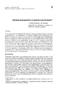
k ∗ ln(n), where k is the number of parameters in the model, n the number of data points, and L is the models data likelihood). Smaller BIC indicate better models. The α and β values yielding the lowest BIC score are used. In estimating α and β, we considered all pairs of non-negative integers such that both values were below 1000. The values of α and β used here were 1 and 177, respectively. These values do not imply that subjects have seen only 1 SC and 177 DOs prior to the experiment, but that only this many observations inform subjects’ prior beliefs about this distribution. The relationship between the choice of the parameters of the beta distribution, α and β, and the BIC of the model used in the parameter estimation is shown in Figure 1.
0.2
confide
deny
0.8
0.6
0.4
0.2
0
10
20
30
Presentation Order
Figure 2: The relationship, for four of the verbs, between the value of p(SC|vi ) given by the model as a function of when in the experiment vi is encountered
BIC
different from the approach commonly taken in psycholinguistics, which is to use static estimates of quantities such as p(SC|vi ) derived from corpora or norming studies. 4.2 a ph Al Beta
Figure 1: The relationship between the BIC of the model used in the parameter estimation step and values of α and β in the beta distribution Because we model subjects’ estimates of p(SC|vi ) in terms of Bayesian inference, with a continuously updated prior, p(SC), the value of p(SC|vi ) depends, in our model, on both verbspecific statistics (i.e. the likelihood p(vi |SC) and the probability of the verb p(vi )) and the point in the experiment at which the trial containing that verb is encountered. We can visualize this relationship in Figure 2, which shows the values given by the model of p(SC|vi ) for four particular different verbs, depending on the point in the experiment at which the verb is seen. The approach we take is hence fundamentally
Analysis
To test whether the model-derived values of p(SC|vi ) are a good fit for the behavioral data, we fit residual reading times at the point of disambiguation using linear mixed effects regression. The model included main effects of p(SC|vi )—as given by the model just described—and complementizer presence, as well as the two-way interaction between these two predictors. Additionally, there were random intercepts of subject and item. p(SC|vi ) was logged and centered at zero. 4.3
Results
There was a highly significant main effect of the posterior probability p(SC|vi ) yielded by the beta-binomial model (β = −40, t = −21.2, p < .001), as well as a main effect of complementizer presence (−4.5, t = −3.7, p < .001). The two-way interaction between complementizer presence and the posterior probability from the beta-binomial model did not reach significance (β = 0.5, t = .5, p > .05). The reason is likely that, in the analysis presented for Study 1, we can interpret the interaction as indicating that when
SC-bias is high, the complementizer has less of an effect; in our model, the posterior probability p(SC|vi ) is both generally higher and has less variance than the same quantity when based on corpus- or norming study estimates, since the prior probability p(SC) is continuously increasing over the course of the experiment. This would have the effect of eliminating or at least obscuring the interaction with complementizer presence. The posterior p(SC|vi ) has a much stronger negative correlation with residual reading times than the measure of SC-bias used in Study 1 (β = −40 as opposed to β = −1.2). 4.4
Discussion
So far, we have replicated a classic finding in the sentence processing literature (Study 1), provided evidence that subjects’ estimates of the conditional probability p(SC|vi ) change based on evidence throughout the experiment, and that this process is captured well by a model which implements a form of incremental Bayesian belief update. We take this as evidence that the language comprehension system is adaptive, in the sense that language users continually update their estimates of probability distributions over syntactic structures.
5
Syntactic Adaptation vs. Motor Adaptation
The results of the model presented in section 4 are amenable to (at least) two explanations. We have hypothesized that, given exposure to new evidence about probability distributions over syntactic structures in English, subjects update their beliefs about these probability distributions, reflected in reading times—a phenomenon we refer to as syntactic adaptation. An alternative explanation, however, is one that appeals to motor adaptation, rather than syntactic adaptation. Specifically, it could be that subjects are simply adapting to the task—rather than to changes in syntactic distributions—as the experiment proceeds, leading to faster reading times. We expect the effect of motor adaptation to be captured by presentation order, or the point in the experiment at which subjects encounter a given stimulus. In particular, we predict a negative correlation between presentation order and reading times. Unfortunately, in the current experiment, presentation order and p(SC|vi ) derived from the Beta-binomial model are positively cor-
related (r = .6)—the latter increases with increasing presentation order, since participants only see SC continuations. The results we observed above could hence also be due to an effect of presentation order. The expected shape of a possible effect of task adaptation is not obvious. That is, it is not clear whether the relationship between presentation order and reading times will be linear. On the one hand, linearity would be the default assumption prior to theoretical considerations about the distributional properties of presentation order. On the other hand, presentation order is a lowerbounded variable, which often are distributed approximately log-normally. Additionally, it is possible that there may be a floor effect: participants may get used to having to press the space bar to advance to the next word and may quickly get faster at that procedure until RTs converge against the minimal time it takes to program the motor movement to press the space bar. Such an effect would likely lead to an approximately log-linear effect of presentation order. We test for an effect of motor adaptation by examining the effect of presentation order on reading times, comparing the effect of linear and logtransformed presentation order. 5.1
Controlling for Presentation Order in the Beta-binomial model
We test for separate effects of syntactic adaptation and motor adaptation by conducting stepwise regressions with two models containing the full factorial design of the Beta-binomial posterior, complementizer presence, and, for the first model, a linear effect of presentation order and, for the second model, log-transformed presentation order. We conducted stepwise regressions using backward elimination, starting with all predictors and removing non-significant predictors (i.e. p > .1), one at a time, until all non-significant predictors are deleted. For both the model including a linear effect of presentation order and a model including logtransformed presentation order, the final models resulting from the stepwise regression procedure included only main effects of complementizer presence and log presentation order. These models are summarized in Figure 1, which includes coefficient-based tests for significance of each of the predictors (i.e. whether the coefficient
is significantly different from zero) as well as χ2 based tests for significance (i.e. the difference between a model with that predictor and one without). Comparing the two resulting models based on the Bayesian Information Criterion, the model containing log-transformed presentation order is a better model than one with a linear effect of presentation order (BIClog = 37467; BICnon−log = 37510). Pres. order untransformed Coef. and χ2 -based tests Predictor
β
p
Comp. pres. Pres. order
−4.3 −.7
< .05 < .001
χ2
p
4.9 28.2
< .05 < .001
Pres. order log-transformed Coef. and χ2 -based tests Predictor
β
p
Comp. pres. Pres. order
−4.3 −33.8
< .05 < .001
χ2
p
4.8 29.4
< .05 < .001
χ2 -based
Table 1: Coefficient- and tests for significance of model resulting from stepwise regression In sum, the beta-binomial derived posterior appears to have no predictive power after presentation order is controlled for. This result does not depend on how presentation order is treated (i.e. log-transformed or not). 5.2
The interaction between SC-bias and presentation order
The results from the previous section suggest that the Beta-binomial derived posterior carries no predictive power after presentation order is controlled for. Is there any evidence at all for syntactic adaptation (as opposed to motor, or task, adaptation)? To attempt to answer this, we analyzed the reading data using the model reported in section 3, with an additional main effect of presentation order, as well as the interactions between presentation order and the other predictors in the model. An overall decrease in reading times due to motor adaptation should surface as a main effect of presentation order, as mentioned; syntactic adaptation, however, is predicted to show up as a twoway interaction between SC-bias and presentation order—since subjects only see SC continuations, subjects should expect this outcome to become more and more probable over the course of the experiment, causing the correlation between SC-bias and reading times to become weaker (thus we pre-
dict the interaction to have a positive coefficient). To test for such an interaction, we performed a stepwise regressions with two models containing the full factorial design of SC-bias, complementizer presence, and, for the first model, a linear effect of presentation order and, for the second model, log-transformed presentation order. The stepwise regression procedure here was identical to the one reported in the previous section. For both models, the remaining predictors were main effects of presentation order, complementizer presence, and SC-bias, as well as a two-way interaction between SC-bias and complementizer presence and a two-way interaction between SCbias and presentation order. The results of these models are given in Table 2. Pres. order untransformed Coef. and χ2 -based tests Predictor
β
p
SC-bias Comp. pres. Pres. order SC-bias:Comp. SC-bias:Pres. Order
−.4 −4.4 −.9 2.6 .1
= < < <