Ising Quantum Chains

arXiv:cond-mat/0611327v1 [cond-mat.stat-mech] 13 Nov 2006

Université Henri Poincaré Faculté des sciences et techniques UFR Sciences et Techniques de la Matière et des Procédés

` Diriger des Recherches Habilitation a

Ising Quantum Chains Dragi Karevski Laboratoire de Physique des Matériaux, UMR CNRS 7556 Soutenance publique le 14 décembre 2005

Membres du jury : Rapporteurs : Pr. Peter Holdsworth, LPS, ENS Lyon Pr. Yurij Holovatch, ICMP, Lviv, Ukraine Pr. Gunter Sch¨ utz, IF, Forschungszentrum J¨ ulich, Allemagne Examinateurs : Pr. Malte Henkel, LPM, UHP Nancy, UMR CNRS 7556 Pr. Wolfhard Janke, ITP, Université de Leipzig, Allemagne Pr. Lo¨ıc Turban, LPM, UHP Nancy, UMR CNRS 7556

Le travail est désormais assuré d’avoir toute la bonne conscience de son cˆ oté : la propension ` a la joie se nomme déj` a “besoin de repos” et commence ` a se ressentir comme un sujet de honte. [...] Oui, il se pourrait bien qu’on en vˆınt ` a ne point céder ` a un penchant pour la vita contemplativa (c’est-` a-dire pour aller se promener avec ses pensées et ses amis) sans mauvaise conscience et mépris de soi-même.

Friedrich Nietzsche Le Gai Savoir

Contents Introduction

5

1 Ising Quantum chain 1.1 Free fermionic models . . . . . . . . . 1.2 Canonical diagonalization . . . . . . . 1.3 Excitation spectrum and eigenvectors 1.3.1 XY -chain . . . . . . . . . . . . 1.3.2 Ising-chain . . . . . . . . . . .

. . . . .

. . . . .

. . . . .

. . . . .

. . . . .

. . . . .

. . . . .

. . . . .

. . . . .

. . . . .

. . . . .

. . . . .

. . . . .

. . . . .

. . . . .

7 7 9 14 14 16

2 Equilibrium behaviour 2.1 Critical behaviour . . . . . . . . . . . 2.1.1 Surface magnetization . . . . . 2.1.2 Bulk magnetization . . . . . . 2.2 Time-dependent correlation functions

. . . .

. . . .

. . . .

. . . .

. . . .

. . . .

. . . .

. . . .

. . . .

. . . .

. . . .

. . . .

. . . .

. . . .

. . . .

19 19 19 22 24

3

Aperiodic modulations 27 3.1 Definition and relevance criterion . . . . . . . . . . . . . . . . . . 27 3.2 Strong anisotropy, weak universality . . . . . . . . . . . . . . . . 28

4 Disordered chains 4.1 Random transverse Ising chain . . . . . . . . . . . . . . 4.1.1 RG-equations . . . . . . . . . . . . . . . . . . . . 4.1.2 Surface behaviour . . . . . . . . . . . . . . . . . 4.1.3 Levy flights . . . . . . . . . . . . . . . . . . . . . 4.2 Inhomogeneous disorder . . . . . . . . . . . . . . . . . . 4.2.1 Definition . . . . . . . . . . . . . . . . . . . . . . 4.2.2 Surface magnetic behaviour . . . . . . . . . . . . 4.2.3 Critical behaviour with relevant inhomogeneity . 4.2.4 Critical behaviour with marginal inhomogeneity

. . . . . . . . .

. . . . . . . . .

. . . . . . . . .

. . . . . . . . .

. . . . . . . . .

33 33 33 35 37 41 41 42 43 44

5 Non-equilibrium behaviour 47 5.1 Equations of motion . . . . . . . . . . . . . . . . . . . . . . . . . 47 5.2 Time-dependent behaviour . . . . . . . . . . . . . . . . . . . . . . 52 5.2.1 Transverse magnetization . . . . . . . . . . . . . . . . . . 52 3

5.2.2 5.2.3 5.2.4 5.2.5

Boundary effects . Two-time functions Critical Ising chain XX chain . . . . .

Discussion and summary

. . . .

. . . .

. . . .

. . . .

. . . .

. . . .

. . . .

. . . .

. . . .

. . . .

. . . .

. . . .

. . . .

. . . .

. . . .

. . . .

. . . .

. . . .

. . . .

. . . .

. . . .

. . . .

55 56 58 59 61

Introduction Quantum spin chains are probably the simplest quantum mechanical systems showing a wide variety of interesting properties [1, 2, 3, 4, 5], a main one being the existence of quantum phase transitions, that is transitions at zero temperature driven by large quantum fluctuations [6]. Singularities occuring strictly [7] at the zero-temperature transition point can, however, produce a typical signature at (very) low temperatures. On the experimental side, physicists are nowadays able to produce artificial samples with behaviour that fits very well with the theoretical descriptions [8, 9, 10]. The low-dimensionality of these systems allows the use of efficient analytical and numerical tools such as the Bethe ansatz [11, 12], bosonization [13, 14], or fermionization [15, 1], exact diagonalization of finite chains or the numerical density matrix (DMRG) approach [16, 17, 18]. We focus our attention in this review on free-fermionic quantum spin chains, which are spin models that can be mapped on systems of non-interacting fermions [1]. The free nature of the elementary excitations allows for an exact diagonalization of the Hamiltonian. It is not here necessary to argue on the usefulness of exact solutions for the implementation of the general comprehension we have of such many-body systems. In particular, they can be used as a garde fou when dealing with more complex systems, unsolved or unsolvable. Moreover, some of the properties they show can still be present in truly interacting systems, that is, models that cannot be or have not yet been mapped on free particles or solvable problems. Most of the studies during the last decades, have been devoted to understand the influence of inhomogeneities [19], such as aperiodic modulation of the couplings between spins [20] or the presence of quenched disorder [21], on the nature of the phase transition [22]. This has culminated in the work of D. Fisher [23] on the random transverse field Ising quantum chain. The extremely broad distribution of energy scales near the critical point, for such random chains, allows the use of a decimation-like renormalization group transformation [24]. Another aspect which is considered in this paper is the non-equilibrium behaviour of such fermionic spin chains. The focus will be on homogeneous systems, since they allow analytical calculations, although expressions are given which are valid for general coupling distributions. The paper is organised as follows: in the two next chapters, we present the general features of the free fermionic spin models and the canonical diagonalization procedure first introduced by Lieb et al. [1]. A detailed discussion is 5

6 given on the excitation spectrum and the associated eigenvectors. It is also pointed out how one can extract the full phase diagram of such spin chains from the knowledge of the surface magnetization. Results on dynamical correlation functions are reviewed. Chapter 3 gives some rapid introduction on the studies done on the aperiodic Ising quantum chain. We have focused the attention on the anisotropic scaling and the weak universality found in such systems. In chapter 4, we present results obtained by ourself and others within the random Ising quantum chain problem. After quickly reviewing RG-results worked out on normal homogeneous distributions of disorder, we present the results obtained on the critical behaviour of random chains with either Lévy type disorder or inhomogeneous disorder. The attention is concentrated on the surface critical behaviour since, due to the particularly simple expression of the surface magnetization, it is possible to obtain many exact results for that quantity. The following chapter deals with the non-equilibrium behaviour. After solving the Heisenberg equations of motion for the basic dynamical variables, we present some aspects of the relaxation of the transverse magnetization. We show that systems with either conserved or non-conserved dynamics present, however, some similarities in their relaxation behaviour. This is illustrated with the XX-chain for conserved dynamics, and with the Ising chain for nonconserved dynamics. Two-time functions are also considered and aging, that is, the dependence of the relaxation process on the age of the system, is also discussed.

Chapter 1

Ising Quantum chain 1.1

Free fermionic models

The generic XY Hamiltonian that we will consider is [25, 26, 27] L−1 L 1 X 1+κ x x 1X z 1−κ y y H =− σn σn+1 + σn σn+1 − hσ 2 n=1 2 2 2 n=1 n

(1.1)

where the σn = 1 ⊗ 1 · · · ⊗ σ ⊗ 1 · · · ⊗ 1 are Pauli matrices at site n and κ is an anisotropy parameter with limiting values κ = 1 corresponding to the Ising case with a Z2 symmetry and κ = 0 describing the XX-model which has U (1) symmetry. We will consider here only free boundary conditions. The phase diagram and the critical behaviour of this model are known exactly since the work of Barouch and McCoy in 1971 [28, 29] who generalized results obtained previously in the case of a vanishing transverse field [1], or at κ = 1 [27]. It was first considered in the framework of conformal invariance [30] in Ref. [31]. In this section, to give a self-consistent presentation, we present in full details the diagonalization procedure, following, more or less closely, the initial work of Lieb et al. [1]. The Hamiltonian can be mapped exactly on a free fermion model, consisting of an assembly of non interacting Fermi-Dirac oscillators. To proceed, let us first introduce the ladder operators σ± =

1 x (σ ± iσ y ) . 2

In the diagonal basis of the σ z component, they simply act as σ + | ↓i = | ↑i and σ − | ↑i = | ↓i. They satisfy the anticommutation rules at same site {σ + , σ − } = 1 7

8

CHAPTER 1. ISING QUANTUM CHAIN

and by construction they commute at different sites. They look like Fermi operators apart that they commute on different sites. True fermionic operators are obtained through a Jordan-Wigner transformation [15]. Consider a basis vector with all spins down (in z-direction) and use the notations |1i ≡ | ↑i and of course |0i ≡ | ↓i, then this state will be the vacuum state destroyed by all the lowering operators σ − : σn− |00 . . . 0i = 0

∀n .

From this vacuum state, all the other states can be built up by applying raising operators σ + . The situation looks very much the same than with fermions. But to have really fermions we need antisymmetry, i. e. anticommutation rules also at different sites. We introduce new operators cn = A(n)σn− , + + c+ n = σn A (n) where A(n) is a unitary operator commuting with σn± : [A(n), σn± ] = 0 . Then automatically we have + − {c+ n , cn } = {σn , σn } = 1

and in particular σnz = 2σn+ σn− − 1 = 2c+ n cn − 1 .

(1.2)

In order to fulfil the antisymmetry principle (sign change under particle exchange), the creation and annihilation operators must satisfy [32] Σl c+ l |n1 , n2 , ..., nl , ...i = (−1) (1 − nl )|n1 , n2 , ..., nl + 1, ...i , cl |n1 , n2 , ..., nl , ...i(−1)Σl nl |n1 , n2 , ..., nl − 1, ...i , Pl−1 where Σl = i=1 ni is the number of particles on the left of the l site. We should find now an operator representation of the sign factor (−1)Σl . It is obvious that the choice l−1 Y (−σiz ) A(l) = i=1

will perfectly do the job [32]. This leads finally to the so called Jordan-Wigner transformations [15] cn =

n−1 Y

(−σiz )σn− =

i=1

n−1 Y i=1

exp iπσi+ σi− σn−

(1.3)

and the adjoint relation. Inverting these relations, we obtain expressions of the ladder operators and the original Pauli matrices in terms of the fermionic creation and annihilation operators c+ and c. Replacing this into our Hamiltonian

1.2. CANONICAL DIAGONALIZATION

9

we obtain the quadratic form H=

L X

1 + + c+ n Anm cm + (cn Bnm cm − cn Bnm cm ) 2 n,m=1

(1.4)

where the real matrices A and B are respectively symmetric and antisymmetric since the Hamiltonian is hermitian. The quadratic nature of the Hamiltonian in terms of the Fermi operators insures the integrability of the model. As in the bosonic case, this form can be diagonalized by a Bogoliubov transformation [1, 33]. Let us mention here briefly that more general quantum spin-1/2 chains are not tractable using this approach. For example, in the Heisenberg model [11] H =J

X

~σn ~σn+1

n

there are terms of the form + z ∝ c+ σnz σn+1 n cn cn+1 cn+1 x leading to interacting fermions. With longer range interactions, such as σnx σn+p , or magnetic fields in the x or y directions, another problem arises due to the non-locality of the Jordan-Wigner transformations. For example a next nearest x neighbour interaction σnx σn+2 generates quartic terms like ν cµn c+ n+1 cn+1 cn+2

where the µ and ν upper-scripts refer to either creation or annihilation operators. In the case of a magnetic field, let us say in the x direction, we have additional terms proportional to the spin operators ! n−1 Y + + x σn = (ci + ci )(ci − ci ) (c+ n + cn ) i=1

which are clearly even worse. Nonlocal effects also appear when dealing with closed boundary conditions [1, 26]. Nevertheless, the Hamiltonian (3.5) is not the most general free-fermionic y x , the expression. We can still add for example terms of the form σnx σn+1 −σny σn+1 so called Dzyaloshinskii-Moriya interaction [34, 35] or play with the boundary conditions [36].

1.2

Canonical diagonalization

We now come to the diagonalization of Hamiltonian (3.5). For that purpose, we express the Jordan-Wigner transformation in terms of Clifford operators [37]

10


Γ1n , Γ2n : Γ1n

n−1 Y

=

Γ2n

= −

−σiz

i=1 n−1 Y i=1

!

−σiz

σnx , !

σny

(1.5)

These operators are the 2L-generators of a Clifford algebra since {Γin , Γjk } = 2δij δnk ,

∀i, j = 1, 2 ; ∀n, k = 1, ..., L

(1.6)

+

and are real operators, that is Γin = Γin . They can be viewed as non-properly normalised Majorana fermions. The different terms in the original Hamiltonian are expressed as σnz = iΓ1n Γ2n x σnx σn+1 = −iΓ2n Γ1n+1 . (1.7) y y σn σn+1 = iΓ1n Γ2n+1 Introducing the two-component spinor 1 Γn Γn = Γ2n one can write the Hamiltonian in the form H=

L−1 L 1 X † y 1X † y Γn σ + iκσ x Γn+1 + Γ hσ Γn , 4 n=1 4 n=1 n

(1.8)

where Γ†n = (Γ1n , Γ2n ) and σy =

0 i

−i 0

σx =

0 1 1 0

are the Pauli matrices, not to be confused with the initial spin operators. Introducing the 2L-component operator Γ† = (Γ†1 , Γ†2 ..., Γ†L ), the Hamiltonian is given by 1 (1.9) H = Γ† TΓ 4 where T is a 2L × 2L hermitian matrix [38, 39] given by   D F 0 ... 0  F† D F 0 ... 0      . . . .. .. ..   0 0   (1.10) T=         0 ... 0 F† D F  0 ... 0 F† D

11

1.2. CANONICAL DIAGONALIZATION with

1 y (σ + iκσ x ) . (1.11) 2 To diagonalize H, we introduce the unitary transformation matrix U build up on the eigenvectors of the T matrix: D = hσ y ,

F=

TVq = ǫq Vq , q = 1, ..., 2L with the orthogonality and completeness relations 2L X

Vq∗ (i)Vq′ (i) = δqq′ ,

2L X

Vq∗ (i)Vq (i′ ) = δii′ .

q=1

i=1

Inserting into (3.12) the expression T = UΛU† where Λpq = ǫq δpq is the diagonal matrix, one arrives at 2L

H=

1 † 1 1X Γ UΛU† Γ = X† ΛX = ǫq x+ q xq 4 4 4 q=1

with the diagonal 2L-component operator X = U† Γ . We introduce now the following parametrisation, which will become clear later, of the eigenvectors Vq :   φq (1)  −iψq (1)     φq (2)    1   Vq = √  −iψq (2)  . (1.12)   . 2 ..     φq (L)  −iψq (L) Utilising this parametrisation, the operators xq and their adjoints are given by L

1 X ∗ φq (i)Γ1i + iψq∗ (i)Γ2i , xq = √ 2 i=1 L

1 X φq (i)Γ1i − iψq (i)Γ2i . x+ q = √ 2 i=1

Now, if we consider the normalised operators 1 dq = √ xq 2

12


we can easily check that together with the adjoints d+ q , they define Dirac Fermions, that is they satisfy the anticommutation rules {d+ q , dq′ } = δq,q′ ,

+ {d+ q , dq′ } = 0 ,

{dq , dq′ } = 0 .

(1.13)

For example, the first bracket is evaluated as {d+ q , dq′ }

=

1X φq (i)φ∗q′ (j){Γ1i , Γ1j } + ψq (i)ψq∗′ (j){Γ2i , Γ2j } 4 i,j

− iψq (i)φ∗q′ (j){Γ2i , Γ1j } + iφq (i)ψq∗′ (j){Γ1i , Γ2j }

and using the anticommutation rules for the Clifford operators and the normalisation of the eigenvectors one is led to the above mentioned result. Finally we have the free fermion Hamiltonian 2L

H=

1X ǫq d+ q dq . 2 q=1

(1.14)

We now take into account the particular structure of the T matrix. Due to the absence of the diagonal Pauli matrix σ z in the expression of T, the non-vanishing elements Tij are those with i + j odd, all even terms are vanishing. This means that by squaring the T matrix we can decouple the original 2L-eigenproblem into two L-eigenproblems. The easiest way to see this is to rearrange the matrix T in the form T=

0 C†

C 0

(1.15)

where the L × L matrix C is given by 

h  Jx   C = −i    

Jy h Jx O

Jy .. .

O .. .

..

..

.

. Jx



      Jy  h

(1.16)

with Jx = (1 + κ)/2 and Jy = (1 − κ)/2. Squaring the T matrix gives1 T2 = 1 The

CC† 0

0 C† C

.

(1.17)

supersymmetric structure appearing in the T 2 matrix has been used in Ref. [40].

13

1.2. CANONICAL DIAGONALIZATION In this new basis the eigenvectors Vq are simply given by   φq (1)  φq (2)      ..   .   1  , φ (L) Vq = √  q  2  −iψ (1)   q     ..   . −iψq (L)

and together with T2 we finally obtain the decoupled eigenvalue equations CC† φq = ǫ2q φq

(1.18)

C† Cψq = ǫ2q ψq .

(1.19)

and Since the CC† and C† C are real symmetric matrices, their eigenvectors can be chosen real and they satisfy completeness and orthogonality relations. This justifies the initial parametrisation of the vectors Vq and one recovers the original formulation of Lieb, Schultz and Mattis [1]. Finally, one can notice another interesting property of the T matrix which is related to the particle-hole symmetry [38]. Due to the off-diagonal structure of T, we have − iCψq = ǫq φq , C† φq = −iǫq ψq

(1.20)

and we see that these equations are invariant under the simultaneous change ǫq → −ǫq and ψq → −ψq . So, to each eigenvalue ǫq ≥ 0 associated to the vector Vq corresponds an eigenvalue ǫq′ = −ǫq associated to the vector   φq (1)  φq (2)      ..   .   1  . φ (L) Vq′ = √  q  2  iψ (1)   q     ..   . iψq (L)

Let us classify the eigenvalues such as ǫq+L = −ǫq

∀q = 1, ..., L

with ǫq ≥ 0 ∀q = 1, ..., L. Then the Hamiltonian can be written as 1 X + d ǫq dq dq − ǫq d+ q+L q+L 2 q=1 L

H=

14


where the operators with q = 1, ..., L are associated to particles and the operators with q = L + 1, ..., 2L are associated with holes, that is negative energy particles. So that, by the usual substitution ηq+ = d+ q ηq+

= dq+L

∀q = 1, ..., L

∀q = 1, ..., L

(1.21)

we rewrite now the Hamiltonian in the form H=

1.3

L L X 1 1X . ǫq ηq+ ηq − ǫq ηq+ ηq − ǫq ηq ηq+ = 2 q=1 2 q=1

(1.22)

Excitation spectrum and eigenvectors

The problem now essentially resides in solving the two linear coupled equations −iCψq = ǫq φq and iC† φq = ǫq ψq . We will present here the solutions of two particular cases, namely the XY -chain without field [1, 26] and the Ising quantum chain in a transverse field [27]. In the following we assume, without loss of generality, that the system size L is even number and κ ≥ 0.

1.3.1

XY -chain

From iC† φq = ǫq ψq , we have the bulk equations 1+κ 1−κ φq (2k − 1) + φq (2k + 1) = 2 2 1+κ 1−κ φq (2k) + φq (2k + 2) = 2 2

−ǫq ψq (2k) −ǫq ψq (2k + 1)

(1.23)

Due to the parity coupling of these equations, we have two types of solutions: φIq (2k) = ψqI (2k − 1) = 0

∀k

(1.24)

and II φII q (2k − 1) = ψq (2k) = 0

∀k

(1.25)

In the first case, the bulk equations that remain to be solved are 1−κ I 1+κ I φq (2k − 1) + φq (2k + 1) = −ǫq ψqI (2k) 2 2 with the boundary conditions φIq (L + 1) = ψqI (0) = 0 . Here we absorb the minus sign in equation (1.23) into the redefinition ψeq = −ψq .

(1.26)

15

1.3. EXCITATION SPECTRUM AND EIGENVECTORS

Using the ansatz φIq (2k − 1) = eiq(2k−1) and ψeqI (2k) = eiq2k eiθq to solve the bulk equations (1.23), we obtain cos q + iκ sin q = ǫq eiθq

that is ǫq = and the phase shift

(1.27)

q cos2 q + κ2 sin2 q ≥ 0

θq = arctan(κ tan q) ,

(1.28) (1.29)

with 0 < θq ≤ 2π to avoid ambiguity. The eigenvectors associated to the positive excitations satisfying the boundary equations are then φIq (2k + 1) = Aq sin (q(2k + 1) − θq ) ψeI (2k) = Aq sin(q2k) ,

(1.30)

q

with

q(L + 1) = nπ + θq

(1.31)

or more explicitly q=

π L+1

1 n + arctan (κ tan q) . π

(1.32)

The normalisation constant Aq is easy to evaluate and is actually dependent on q. Using θq = q(L + 1) + nπ, one can write φIq in the form φIq (2k + 1) = −Aq δq sin q(L − 2k) , where δq = (−1)n is given by the sign of cos q(L + 1). The equation (1.32) has L/2 − 1 real solutions, that in the lowest order in 1/L are given by qn ≃

π (n − νn ) L

(1.33)

with

nπ L 1 n , n = 1, 2, ..., − 1 . − arctan κ tan L π L 2 There is also a complex root of (1.32) νn =

q0 =

π + iv 2

(1.34)

(1.35)

where v is the solution of tanh v = κ tanh[v(L + 1)] . With the parametrisation x = e−2v and ρ2 = x=

1−κ 1+κ ,

ρ2 1−

xL (1

− ρ2 x)

(1.36)

one is led to the equation

16


and the first nontrivial approximation leads to x−1 ≃ ρ−2 − (1 − ρ4 )ρ−2(L−1) .

(1.37)

The excitation associated with this localised mode (see the form of φq0 and ψq0 with q0 = π/2 + iv) is exponentially close to the ground state, that is ǫq0 ≃ (1 + ρ2 )ρL .

(1.38)

From this observation, together with some weak assumptions, the complete phase diagram of the system can be obtained. We will discuss this point later. The solutions of the second type satisfy the same bulk equations but the II difference lies in the boundary conditions φII q (0) = ψq (L + 1) = 0. The eigenvectors are given by

with

φII q (2k) = Aq sin(q2k) ψeqII (2k + 1) = Aq sin(q(2k + 1) + θq ) = −Aq δq sin q(L − 2k) , π q= L+1

1 n − arctan (κ tan q) π

(1.39)

(1.40)

which has L/2 real roots. To the leading order, one gets qn =

π (n − νn ) L

(1.41)

with

nπ L 1 n , n = 1, 2, ..., + arctan κ tan L π L 2 which completes the solution of the XY -chain. νn =

1.3.2

(1.42)

Ising-chain

The solution of the Ising chain (κ = 1) proceeds along the same lines [27]. The bulk equations are (1.43) hφq (k) + φq (k + 1) = ǫq ψeq (k)

with the boundary conditions

φq (L + 1) = ψq (0) = 0 .

(1.44)

With the same ansatz as before, one arrives at h + eiq = ǫq eiθq that is ǫq = and

(1.45)

q (h + cos q)2 + sin2 q

θq = arctan

sin q h + cos q

.

(1.46) (1.47)

1.3. EXCITATION SPECTRUM AND EIGENVECTORS

17

Taking into account the boundary conditions, the solutions are readily expressed as φq (k) = A sin(qk − θq ) (1.48) ψq (k) = −A sin(qk) where q is a solution of the equation 1 sin q π n + arctan . q= L+1 π h + cos q

(1.49)

The eigenvectors can then also be written in the form φq (k) = −A(−1)n sin(q(L + 1 − k)) . ψq (k) = −A sin(qk)

(1.50)

In the thermodynamic limit, L → ∞, for h ≥ 1, the equation (1.49) gives rise to L real roots. On the other hand, for h < 1, there is also one complex root q0 = π + iv associated to a localised mode such that v is solution of tanh(v(L + 1)) = −

sinh v . h − cosh v

(1.51)

To the leading order, we have v ≃ ln h. The eigenvectors associated to this localised mode are φq0 (k) = A(−1)k sinh(v(L + 1 − k)) ψq0 (k) = −A(−1)k sinh(vk) .

(1.52)

Exactly at the critical value h = 1, we have θq = q/2, which gives a simple quantisation condition: q=

2nπ , n = 1, 2, ..., L 2L + 1

(1.53)

Changing q into π − q, we have [41] φq (k) = ψq (k) =

√ 2 (−1)k+1 cos(q(k 2L+1 2 √ (−1)k sin(qk) , 2L+1

− 1/2))

(1.54)

and

q ǫq = 2 sin , 2 with q = (2n + 1)π/(2L + 1) and n = 0, 1, ..., L − 1.

(1.55)

18


Chapter 2

Equilibrium behaviour 2.1

Critical behaviour

From the knowledge of the eigenvectors φ and ψ, and the corresponding oneparticle excitations, we can in principle calculate all the physical quantities, such as magnetization, energy density or correlation functions. However, they are, in general, complicated many-particles expectation values due to the non-local expression of the spin operators in terms of fermions. We will come later to this aspect when considering the dynamics. Nevertheless, quantities that can be expressed locally in terms of fermion are simple, such as correlations involving only σ z operators or σ1x .

2.1.1

Surface magnetization

A very simple expression is obtained for the surface magnetization, that is the magnetization on the x (or y) direction of the first site. The behaviour of the first spin [42, 43] gives general informations on the phase diagram of the chain [28, 29, 30]. Since the expectation value of the magnetization operator in the ground state vanishes, we have to find a bias. The usual way will be to apply a magnetic field in the desired direction, in order to break the ground state symmetry. Of course this procedure has the disadvantage to break the quadratic structure of the Hamiltonian. Another route is to extract the magnetization behaviour from that of the correlation function. In this respect, the x(y) component of the surface magnetization is obtained from the autocorrelation function G(τ ) = hσ1x (0)σ1x (τ )i in imaginary time τ where σ1x (τ ) = eτ H σ1x e−τ H . Introducing the diagonal basis of H, we have X |hi|σ1x |0i|2 e−τ (Ei −E0 ) (2.1) G(τ ) = |hσ|σ1x |0i|2 e−τ (Eσ −E0 ) + i>1

where |0i is the ground state with energy E0 and |σi = η1+ |0i is the first excited state with one diagonal fermion whose energy is Eσ = E0 + ǫ1 . From the 19

20

CHAPTER 2. EQUILIBRIUM BEHAVIOUR

previous section we see that we have a vanishing excitation for h < 1 in the thermodynamic limit L → ∞ leading to a degenerate ground state. This implies that in the limit of large τ , only the first term in the previous expression of the autocorrelation function contributes: lim G(τ ) = [mxs ]2 ,

(2.2)

τ →∞

where mxs = hσ|σ1x |0i. Noticing that σ1x = Γ11 = c+ 1 + c1 and making use of the P 1 inverse expression, Γn = q φq (n)(ηq+ + ηq ), one obtains mxs = hσ|σ1x |0i = φ1 (1) .

(2.3)

Similarly, one can obtain mys = hσ|σ1y |0i = ψ1 (1). Following Peschel [42], it is now possible to obtain a closed formula for the surface magnetization [43]. In the semi-infinite limit L → ∞, for h < 1, the first gap Eσ − E0 = ǫ1 vanishes due to spontaneous symmetry breaking. In this case, equations (1.20) simplify into C† φ1 = 0 . Cψ1 = 0

(2.4)

Noticing that changing κ into −κ, mx and my are exchanged, in the following we will consider only the x-component. To find the eigenvector φ1 , we rewrite C† φ1 = 0 in the iterative form φ1 (n + 1) φ1 (n) = Kn (2.5) φ1 (n) φ1 (n − 1) where Kn is a 2 × 2 matrix associated to the site n whose expression for homogeneous coupling constants is 2h 1−κ 1+κ 1+κ . (2.6) Kn = K = − −1 0 By iterations, we obtain for the (n + 1)th component of the eigenvector φ1 the expression φ1 (n + 1) = (−1)n φ1 (1) (Kn )11 (2.7) where the indices 11 stand forP the 1,1 component of the matrix Kn . The normalisation of the eigenvector, i φ21 (i) = 1, leads to the final expression [43] mxs

"

= 1+

∞ X

n=1

n

2

|(K )11 |

#−1/2

.

(2.8)

First we note that the transition from a paramagnetic to an ordered phase is characterised by the divergence of the sum entering (2.8). On the other hand, since for a one-dimensional quantum system with short-range interactions, the surface cannot order by itself, the surface transition is the signal of a transition

21

2.1. CRITICAL BEHAVIOUR

in the bulk. It means that one can obtain some knowledge of the bulk by studying surface quantities. To do so, we first diagonalize the K matrix. The eigenvalues are i p 1 h h ± h2 + κ2 − 1 (2.9) λ± = 1+κ

for h2 + κ2 > 1 and complex conjugates otherwise

i p 1 h h ± i 1 − h2 − κ2 ρ exp(±iϑ) (2.10) 1+κ p √ with ρ = (1 − κ)/(1 + κ) and ϑ = arctan( 1 − h2 − κ2 /h) and they become degenerate on the line h2 + κ2 = 1. The leading eigenvalue gives the behaviour of φ21 (n) ∼ |λ+ |2n which, for an ordered phase, implies that |λ+ | < 1. The first mode is then localised near the surface. From this condition on λ+ , we see that it corresponds to h < hc = 1. For h > 1, the surface magnetization exactly vanishes and we infer that the bulk is not ordered too. So that for any anisotropy κ, the critical line is at h = 1 and in fact it belongs to the 2d-Ising [44] universality class.1 As it is shown hereafter, the special line h2 + κ2 = 1, where the two eigenvalues collapse, separates an ordinary ferromagnetic phase (h2 + κ2 > 1) from an oscillatory one (h2 + κ2 < 1) [28]. This line is known as the disorder line of the model. The line at vanishing anisotropy, κ = 0, is a continuous transition line (with diverging correlation length) called the anisotropic transition where the magnetization changes from x to y direction. In the ordered phase, the decay of the eigenvector φ1 gives the correlation length of the system, which is related to the leading eigenvalue by n (2.11) φ21 (n) ∼ |λ+ |2n ∼ exp − ξ λ± =

so that

1 . 2| ln |λ+ ||

(2.12)

mxs ∼ (1 − h)1/2

(2.13)

ξ=

By analysing λ+ , it is straightforward to see that the correlation length exponent defined as ξ ∼ δ −ν , with δ ∝ 1 − h for the Ising transition and δ ∝ κ for the anisotropic one, is ν = 1. Of course, a specific analysis of formula (2.8) leads to the behaviour of the surface magnetization. At fixed anisotropy κ, close enough to the Ising transition line we have

giving the surface critical exponent βsI = 1/2. In the oscillatory phase, a new length scale appears given by ϑ−1 . A straightforward calculation gives for the 1 To get an account on the connection between d-dimensional quantum systems and d + 1dimensional classical systems, on can refer to Kogut’s celebrated review [45]. The idea lies in the fact that, in imaginary (Euclidean) time τ , the evolution operator e−τ H , where H is the Hamiltonian of the d-dimensional quantum system, can be interpreted as the transfer matrix of a d + 1 classical system.

22


eigenvector φ1 the expression φ1 (n) = (−1)n ρn

1+κ sin(nϑ)φ1 (1) h tan ϑ

(2.14)

which leads to βsa

mxs ∼ κ1/2

(2.15)

close to the anisotropy line, so = 1/2 too. We have seen here how from the study of surface properties [43] one can determine very simply (by the diagonalization of a 2 × 2 matrix) the bulk phase diagram and also the exact correlation length [28]. One may also notice that expression (2.8) is suitable for finite size analysis [46], cut off at some size L. In fact for the Ising chain, to be precise, one can work with symmetry breaking boundary conditions [47]. That is, working on a finite chain, we fix the spin at one end (which is equivalent to set hL = 0) and evaluate the magnetization on the other end. In this case, the surface magnetization is exactly given by (2.8) where the sum is truncated at L − 1. The fixed spin at the end of the x chain, let us say σL = +, leads to an extra Zeeman term since we have now in x the Hamiltonian the term − JL−1 2 σL−1 , where the last coupling JL−1 plays the role of a magnetic field. The vanishing of hL induces a two-fold degeneracy of the Hamiltonian which is due to the exact vanishing of one excitation, say ǫ1 . x This degeneracy simply reflects the fact that [σL , H] = 0. On a mathematical ground, we can see this from the form of the T matrix which has a bloc-diagonal structure with a vanishing 2 × 2 last bloc. From the vacuum state associated to the diagonal fermions, |0i, and its degenerate state η1+ |0i, we can form the two ground states 1 |±i = √ |0i ± η1+ |0i (2.16) 2 x x associated respectively to σL = + and σL = −. Since we have a boundary symmetry breaking field, we can directly calculate the surface magnetization from the expectation value of σ1x in the associated ground state. It gives h+|σ1x |+i = φ1 (1), where φ1 (1) is exactly obtained for any finite size from C† φ1 = 0. This finite-size expression has been used extensively to study the surface properties of several inhomogeneous Ising chains with quenched disorder [48, 49, 50, 51], where a suitable mapping to a surviving random walk [47] problem permits to obtain exact results.

2.1.2

Bulk magnetization

As stated at the beginning of this section, quantities involving σ x or σ y operators are much more involved. Nevertheless, thanks to Wick’s theorem, they are computable in terms of Pfaffians [52, 28] or determinants whose size is linearly increasing with the site index. For example, if one wants to compute hσ|σlx |0i, the magnetization at site l, one has to evaluate the expectation value [53] ml = hσ|σlx |0ih0|η1 A1 B1 A2 B2 . . . Al−1 Bl−1 Al |0i ,

(2.17)

23

2.1. CRITICAL BEHAVIOUR

where we have defined Ai = Γ1i and Bi = −iΓ2i in order to absorb unnecessary i factors. These notations were initialy introduced by Lieb et al [1]. Note that B 2 = −1. Since Al and Bl are linear combinations of Fermi operators: Al =

X q

φq (l) ηq+ + ηq ,

Bl =

X q

ψq (l) ηq+ − ηq ,

(2.18)

we can apply Wick’s theorem for fermions [1]. The theorem states that we may expand the canonical (equilibrium) expectation value, with respect to a bilinear fermionic Hamiltonian, of a product of operators obeying anticommutation rules, in terms of contraction pairs. For example, if we have to evaluate the product hC1 C2 C3 C4 i, we can expand it as hC1 C2 C3 C4 i = hC1 C2 ihC3 C4 i − hC1 C3 ihC2 C4 i + hC1 C4 ihC2 C3 i . Due to the fermionic nature of the operators involved, a minus sign appears at each permutation. In our case, it is easy to see that the basic contractions h0|Ai Aj |0i and h0|Bi Bj |0i are vanishing for i 6= j. The only contributing terms are those products involving only pairs of the type h0|η1 A|0i, h0|η1 B|0i or h0|BA|0i. One may also remark that it is unnecessary to evaluate terms of the form h0|η1 B|0i since in this case there is automatically in the product a vanishing term h0|Ai Aj |0i with i 6= j. The simplest non-vanishing product appearing in the Wick expansion is h0|η1 A1 |0ih0|B1 A2 |0i . . . h0|Bl−1 Al |0i . The local magnetization ml is then given by the l × l determinant [53, 47]

with

ml =

H1 H2 .. .

G11 G21 .. .

G12 G22 .. .

... ...

G1l−1 G2l−1 .. .

Hl

Gl1

Gl2

...

Gll−1

Hj = h0|η1 Aj |0i = φ1 (j) and Gjk = h0|Bk Aj |0i = −

X

φq (j)ψq (k) .

(2.19)

(2.20)

(2.21)

q

This expression for the local magnetization enables to compute, at least numerically, magnetization profiles [54, 55] and to extract scaling behaviour. For example far in the bulk of the Ising chain we have near the transition the power law behaviour mb ∼ (1 − h)1/8 for h < 1 and zero otherwise [27]. To conclude this section, one can also consider more complicated quantities such as two-point correlation functions [1, 27] in the same spirit.

24

2.2


Time-dependent correlation functions

Time-dependent correlations functions are of primary importance since experimentally accessible dynamical quantities are, more or less simply, related to them. For general spin chains, the exact analysis of the long time behaviour of spin-spin correlations is a particularly difficult task. The generic time-dependent spin-spin correlation function is hσiµ (t)σjν i where i, j are space indices, µ, ν = x, y, z and where the average h . i ≡ T r{ . e−βH }/T r{e−βH } is the canonical quantum expectation at temperature T = 1/β. The time-dependent operator σiµ (t) = eiHt σiµ e−iHt is given by the usual Heisenberg representation. Most of the approximation schemes developed so far [56, 57] are not really relevant for such many-body systems, at least at finite temperature. One is ultimately forced to go on numerical analyses, basically by exact diagonalization of very short chains, although recently there has been a significant numerical progress using time-dependent DMRG (Density Matrix Renormalization Group) procedure [58]. Nontrivial exact solutions for time-dependent correlations do exist for free fermionic spin chains [59, 60, 61, 29, 62, 63]. due to the non-interacting nature of the excitations. For such chains, not only bulk regimes were investigated but also boundary effects [64, 65, 66, 67, 68]. On one hand, the z − z correlations are easily calculable due to their local expression in terms of the Fermi operators. They are basically fermion density correlation function. On the other hand, the x − x correlations are much more involved since in the Fermi representation one has to evaluate string operators. Nevertheless, as for the static correlators, one may use Wick’s theorem to reduce them to the evaluation of a Pfaffian, or determinant, whose size is linearly increasing with i + j. For the N -sites free boundary isotropic XY -chain in a transverse field, H=

N −1 N hX z J X x x x (σj σj+1 + σjx σj+1 )− σ , 4 j=1 2 j=1 j

the basic contractions at inverse temperature β are given by [64]: P βε hAj (t)Al i = N2+1 q sin qj sin ql cos εq t − i sin εq t tanh 2 q P βε hAj (t)Bl i = N2+1 q sin qj sin ql i sin εq t − cos εq t tanh 2 q

(2.22)

and the symmetry relations

hBj (t)Bl i = −hAj (t)Al i hBl (t)Aj i = −hAj (t)Bl i

(2.23)

where the excitation energies εq = J cos q−h with q = nπ/(N +1) , n = 1, . . . , N . With the help of these expressions, one is able to evaluate the desired timedependent correlations, at least numerically.

2.2. TIME-DEPENDENT CORRELATION FUNCTIONS

25

The z − z correlator, namely hσjz (t)σlz i, is given in the thermodynamic limit at infinite temperature T = ∞ by [69, 64] 2 hσjz (t)σlz i Jj−l (Jt) − (−1)l Jj+l (Jt)

(2.24)

where Jn is the Bessel function of the first kind. One has to notice that this result is field independent. The bulk behaviour is obtained by putting j, l → ∞ and keeping l − j finite. One has Jt≫1

2 hσjz (t)σlz i = Jj−l (Jt) ∼ t−1 ,

(2.25)

leading to a power law decay in time. For large time, the boundary effects lead to πr i 2 8 h 2 Jt − l (l + r)2 (2.26) sin hσjz (t)σlz i ≃ πJ 3 t3 2 with r = j − l the distance between the two sites. Therefore, the decay in time changes from t−1 to t−3 near the boundaries [64]. In the low-temperature limit (T = 0), we have a closed expression for h ≥ J which is time and site independent [64]: hσjz (t)σlz i = 1

(2.27)

revealing an ordered ground state. This can be related to the fact that the ground state corresponds to a completely filled energy-band, since all the energy excitations are negative. As already stated before, the calculation of the z − z correlation function is an easy task and we will not go on other models. In order to calculate the x − x time dependent correlation functions for such free-fermionic chains, one has to evaluate hσjx (t)σlx i = hA1 (t)B1 (t) . . . Aj−1 (t)Bj−1 (t)Aj (t)A1 B1 . . . Al−1 Bl−1 Al i . (2.28) In the high temperature limit (T = ∞), the bulk correlation function of the isotropic XY chain in a transverse field h is given by the Gaussian behaviour [70, 59, 60]: J 2 t2 hσjx (t)σlx i = δjl cos ht exp − (2.29) 4 where δjl is the Kronecker symbol. The boundary effects are hard to be taken into account due to the fact that the Pfaffian to be evaluated is a Toeplitz determinant [71, 59, 72] that can be treated only for large order [59]. Nevertheless for a vanishing transverse field, a conjecture was inferred from exact calculations for the boundary nearest sites i = 1, 2, . . . , 5, claiming an asymptotic power-like decay [65]: hσjx (t)σlx i ∼ δjl t−3/2−(j−1)(j+1) . (2.30) At vanishing temperature and for h ≥ J, the basic contractions can be evaluated in a closed form too. This leads to [73, 74, 64, 62] hσjx (t)σlx i = exp(−iht) exp[i(j − l)]Jj−l (Jt)

(2.31)

26


for the bulk correlation function. The Bessel function gives rise to a t−1/2 asymptotic behaviour. So moving from T = ∞ to T = 0 there is a dramatic change in the time decay behaviour [64]. Finally, one is also able to take into account the free boundary effects. In this case, for large enough time, the behaviour changes from t−1/2 to t−3/2 [64]. At finite temperature the asymptotic decay of the time-dependent correlators is exponential [75]: 2

2

x hσix (t)σi+n i ∝ t2(ν+ +ν− ) exp f (n, t)

(2.32)

where f (n, t) is a negative monotonically decreasing function with increasing T . The preexponents ν± are known functions [75] of the field h, the temperature and the ratio n/t. When T → ∞, the function f (n, t) diverges logarithmically indicating the change of the decay shape from exponential to Gaussian [66]. To end this section, one may mention that the decay laws for the x − x time-dependent correlation functions of the anisotropic XY chain are basically the same as for the isotropic case, namely power law at zero temperature and Gaussian at infinite temperature [72].

Chapter 3

Aperiodic modulations 3.1

Definition and relevance criterion

Since the discovery of quasicrystals in the middle of the eighties [76], extensive studies on Ising quantum chains with quasiperiodic or aperiodically modulated couplings have been done in the nineties [77, 78, 79, 53, 39], see also [80] for a review. The interest in the field of critical phenomena in such aperiodic quantum chains lied in the fact that they offered intermediate situations between pure and random cases. Let us first define the aperiodic modulation itself. Most of the aperiodic sequences considered were generated via inflation rules by substitutions on a finite alphabet, such that A → S(A), B → S(B), ..., where S(A)(S(B)) is a finite word replacing the letter A(B). Starting from an initial letter and generating the substitution ad eternam, one obtains an infinite sequence of letters to whom a coupling sequence of the chain can be associated by the rules A → JA , B → JB , ... If one considers a two letter sequence then the cumulated deviation ∆(L) from the average coupling J at a length scale L is characterized by a wandering exponent ω such that ∆(L) =

L X i=1

(Ji − J) ∼ δLω

(3.1)

where δ is the strength of the aperiodic modulation and where the wandering exponent ω is obtained from the substitution matrix M whose elements (M )ij give the number of letters aj contained in the word S(ai ) [81, 82]. The wandering exponent is given by ln |Λ2 | ω= (3.2) ln Λ1 where Λ1 and Λ2 are the largest and next largest eigenvalues of the subsitution matrix. Near the critical point of the pure system, the aperiodicity introduces a shift of the critical coupling δt ∼ ξ ω−1 ∼ t−ν(ω−1) which has to be compared 27

28

CHAPTER 3.

APERIODIC MODULATIONS

to the distance to criticality t [20]. This leads to Luck’s criterion δt ∼ t−Φ t

Φ = 1 + ν(ω − 1)

(3.3)

and in the Ising universality class since ν = 1, one obtains Φ=ω.

(3.4)

When ω < 0, the perturbation is irrelevant and the system is in the Onsager universality class. On the other hand for ω > 0, the fluctuations are unbounded and the perturbation is relevant. For ω = 0, that is in the marginal case, one may expect continuously varying exponents.

3.2

Strong anisotropy, weak universality

It is not here the purpose to give an exhaustive view on what was done in the context of aperiodic modulation of the Ising quantum chain, but rather to exemplify some (simple) aspects of it which have not really been noticed before (as far as my knowledge goes). The Ising quantum chain in a transverse field is defined by the hamiltonian: H=−

L−1 L 1X 1X x Ji σix σi+1 − hi σiz , 2 i=1 2 i=1

(3.5)

where the σ’s are the Pauli spin operators and Ji , hi are inhomogeneous couplings. In marginal aperiodic systems, for which hi = h and λi = λRfi with λi = Ji /hi and fi = 0, 1 generating the aperiodicity, an anisotropic scaling was found. For such systems, the smallest excitations scale at the bulk critical point as Λ ∼ L−z with the size L of the chain. In the marginal aperiodic case, it was shown numerically that the anisotropy exponent z is continuously varying with the control parameter R [83, 53] z(R) = xms (R) + xms (R−1 ) ≥ 1 ,

(3.6)

where xms (R) is the magnetic exponent associated to ms = hσ1x i.1 The observed symmetry in the exchange R ↔ 1/R in (3.6) was demonstrated in [79] for aperiodic systems generated by inflation rules, using a generalization of an exact renormalization group method introduced first in [38] and applied to several aperiodic systems in [39]. We show here that this equation comes from a relation, valid for any distribution of couplings leading to anisotropic scaling, that rely the first gap Λ1 to the surface magnetization. Using a Jordan-Wigner transformation [1], the hamiltonian (3.5) can be rewritten in a quadratic form in fermion operators. It is then diagonalized by a 1 One may notice that relation (3.6) holds for the homogeneous system, R = 1, with xms = 1/2 and z = 1.

29

3.2. STRONG ANISOTROPY, WEAK UNIVERSALITY canonical transformation and reads H=

L X

1 Λq (ηq† ηq − ) , 2 q=1

(3.7)

where ηq† and ηq are the fermionic creation and anihilation operators. The one fermion excitations Λq satisfy the following set of equations: Λq Ψq (i) = −hi Φq (i) − Ji Φq (i + 1)Λq Φq (i) = −Ji−1 Ψq (i − 1) − hi Ψq (i) (3.8) with the free boundary condition J0 = JL = 0. The vectors Φ and Ψ are related to the coefficients of the canonical transformation and enter into the expressions of physical quantities. For example the surface magnetization, ms = hσ1x i, is simply given by the first component of Φ1 associated to the smallest excitation of the chain, Λ1 . Let us consider now a distribution of the couplings which leads to anisotropic scaling with a dynamical exponent z > 1, as it is the case for bulk marginal aperiodic modulation of the couplings [83, 53, 79, 38, 39]. Then the bottom spectrum of the critical hamiltonian scales as Λq ∼ L−z in a finite size system. According to Ref.[79, 38, 39], the asymptotic size dependence of Λ1 (L) is given by the expressions −1  L−1 i L−1 X Y Y Ψ (1) 1  (3.9) λ−2 λ−1 1 + Λ1 (L) ≃ (−1)L L−j Φ1 (L) i=1 i i=1 j=1 −1  L−1 i L−1 X Y Y Φ (L) 1  Λ1 (L) ≃ (−1)L λ−2 , λ−1 1 + j Ψ1 (1) i=1 i i=1 j=1

(3.10)

which are valid at the critical point and in the ordered phase. Noting in (3.9) that −1  −1  L−1 i L−1 i L−1 L−1 XY XY Y Y  = 1 + λ2j  λ−2 λi 1 + , (3.11) λ−1 i L−j i=1

i=1 j=1

i=1 j=1

i=1

equation (3.9) becomes

−1  i L−1 L−1 XY Y Ψ (1) 1 Λ1 (L) ≃ (−1)L λ2j  . λi 1 + Φ1 (L) i=1 i=1 j=1

(3.12)

Now multiplying both sides of equation (3.12) with (3.10) leads to 

Λ1 (L) ≃ 1 +

L−1 X

i Y

i=1 j=1

−1/2 

 λ−2 j

1 +

L−1 X

i Y

i=1 j=1

−1/2

λ2j 

.

(3.13)

30

CHAPTER 3.


which is symmetric under the exchange λ ↔ 1/λ. One recognizes in this expresh i−1/2 PL−1 Qi sion the surface magnetization [42] ms (L, {λi }) = 1 + i=1 j=1 λ−2 of j the quantum chain, so that one finally obtains Λ1 (L) ≃ ms (L, {λi })ms (L, {λ−1 i }) .

(3.14)

This relation connects a bulk quantity, Λ1 , with surface quantities, namely ms (L, {λi }) and the surface magnetization of the dual chain, ms (L, {λ−1 i }). Consider now a deterministic distribution of the chain couplings, {λi }, with hi = h and λi = JRfi /h with fi following some sequence of 0 and 1. The QL 1/L = 1 [27] critical coupling λc follows from the relation limL→∞ k=1 (Jk /hk ) −ρ∞ and gives λc = R with ρ∞ the asymptotic density of modified couplings λR. The modulation of the couplings introduces a perturbation which can be either relevant, marginal or irrelevant. For the Ising quantum chain the fluctuations ¯ at a length scale L ∆(L) = PL (λk − λ) ¯ ∼ Lω around the average coupling λ k=1 governs the relevance of the perturbation [20]. According to Luck’s criterion, if ω < 0 the fluctuations are bounded and the system is in the Ising universality class. On the other hand for ω > 0, the fluctuations are unbounded and one has to distinguish two differentPsituations. The evaluation of the surface L magnetization is related to the sum j=1 λ−2j R−2nj where nj is the number of modified couplings,PλR, at size j. At the critical point, the sum can be rewritten ω L asymptotically as j=1 R−2Bj . Now assume that the coefficient B is positif (if not the roles of R > 1 and R < 1 are reversed in the following discussion). For R > 1 the previous sum is absolutely convergent for L → ∞ and leads to a finite surface magnetization with exponentially small corrections in a finite size system. On the other hand for R < 1, the sum is diverging exponentially and the surface magnetization is governed by the dominant term exp(−2B ln RLω ), so that ms (L, R) ∼ exp (−A(R)Lω ) , (3.15) with A(R) > 0. So from equation (3.14), in both case (R > 1 or R < 1) the first gap Λ1 will show an essential singularity leading to z = ∞: ω ˜ , (3.16) Λ1 (R, L) ∼ exp −A(R)L

˜ ˜ with A(R) = A(R) for R < 1 and A(R) = A(1/R) for R > 1 since from (3.14) Λ1 (R) = Λ1 (1/R). In the marginal case, corresponding to ω = 0, that is a logarithmic divergence of the fluctuations, nj ≃ ρ∞ j + C ln j where C is some constant, it can be shown that the surface magnetization scales at the critical point as ms (L, {λi }c ) ∼ L−xms (R)

(3.17)

with an exponent xms (R) varying continuously with the control parameter R. In fact the sum can be evaluated at the critical point using nj ≃ ρ∞ j + C ln j. RL P P −2C ln j −2j −2nj dx x−2C ln R ∼ L1−2C ln R . ≃ L ∼ One obtains L R j=1 R j=1 λc

3.2. STRONG ANISOTROPY, WEAK UNIVERSALITY

31

This expression is only valid in the weak perturbation regime for R ≃ 1, that is in first order in ln R. For a stronger regime one has to retain higher terms in the nj expression. At this order, the surface magnetic exponent is xms (R) ≃ 1/2 − C ln R. One can remark that for a sequence like the period-doubling one [83, 53], xms (R) = xms (1/R) which implies C = 0 (one can test this numerically) and then the former calculation gives xms (R) = 1/2 + O(ln2 R). Finally, from (3.14) and (3.17) one obtains the relation z(R) = xms (R) + xms (R−1 ) .

(3.18)

The anisotropy exponent z is then given by one surface magnetic exponent xms which is a function of the perturbation strength. The symmetry R ↔ 1/R of z is due to the self-duality of the Ising quantum chain which implies for all bulk quantities the relation Q({λi }) = Q({λ−1 i }). For a symmetric distribution of couplings with respect to the center of the chain, leading to xms (R) = xms (1/R) (see the period-doubling case [83, 53, 79, 38, 39]), one observes a weak universality for the surface critical behaviour. The −z bottom of the spectrum scales anisotropically as Λ ∼ L−z ∼ ξ⊥ ∼ tzν where t measures the deviation from the critical point and ν = 1 is the exponent of the longitudinal correlation length ξ⊥ . So that from (3.14) ms (t) ∼ (tz )

1/2

.

(3.19)

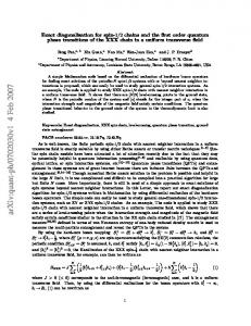
From anisotropic scaling, one obtains for the critical dimension of the surface energy density es the scaling relation xes = z + 2xms . Using the symmetry of xms one has 2 es ∼ (tz ) . (3.20) We see that we recover the homogeneous surface exponents xms = 1/2, xes = 2 when the deviation from the critical point is mesured with tz ∼ Λ1 . The same weak universality seems to hold for the bulk quantities. In fact, it was shown in Ref.[53] that the bulk energy density scales as e ∼ L−z for marginal aperiodic modulation of the couplings. So again the pure energy density exponent xe = 1 is recovered. Here we P have investigated the behaviour of the mean bulk magnetization mb = 1/L i m(i) for the period-doubling sequence from finite size scaling analysis. The magnetization is evaluated at the bulk critical point for sizes up to L = 1024. Numerically the profiles are well rescaled on the same curve with the exponent xmb (R) = z(R)/8 but we notice that as the size increases the profiles are more and more decorated with a growing fluctuation amplitude. This suggeres that the finite size behaviour of the mean critical magnetization is given by: 1/8 . (3.21) mb ∼ L−z/8 ∼ L−z On the basis of the numerical datas, the magnetization profile is compatible with the form m(l, L) = L−z/8 |sin(πl/L)|xms −xmb [A + G(l/L)] ,

(3.22)

32

CHAPTER 3.

2.5


0.8

m(l,L)

0.6

2.0

0.4

m(l,L) L

z/8

0.2 0.0

1.5

0.0

0.2

0.4

0.6

0.8

1.0

l/L

1.0

0.5

0.0

L=16 L=64 L=256 L=1024

0.0

0.2

0.4

0.6

0.8

1.0

l/L

Figure 3.1: Rescaled magnetization profiles of the period-doubling chain with r = 5. The insert gives the corresponding magnetization profile. where A is a constant and G(x) is a kind of fractal Weierstrass function with zero mean value whose fourier momentum are given by the period-doubling cascade. The sinus term is very general for the profiles of the Ising quantum chains and is related to the geometry of the system. This can be demonstrated explicitely for the pure case [54] and was obtained numerically for random Ising systems [84]. The only difference here is that we have not only a pure constant in the front of it but in addition a fractal function of zero mean which controles the local fluctuations, due to the aperiodic distribution, around some average environnement. In conclusion the weak universality observed in this systems implies that the knowledge of the anisotropy exponent z is sufficient to determine the critical behaviour of the system.

Chapter 4

Disordered chains 4.1 4.1.1

Random transverse Ising chain RG-equations

Quenched disorder, i.e., time-independant disorder, has a strong influence on the nature of phase transitions and in particular on quantum phase transition. Many features of the randomness effects can be observed in one-dimensional systems, for which several exact results have been obtained and a general scenario (infinit randomness fixed point) has been developped [85]. In particular, since the work of Fisher [23], the 1d random transverse Ising model has been the subject of much interest. The model is defined via the Hamiltonian: H=−

L−1 L 1X 1X x Ji σix σi+1 − hi σiz , 2 i=1 2 i=1

(4.1)

where the exchange couplings, Ji and transverse fields, hi , are random variables. In the case of homogeneous independently distributed couplings and fields, Fisher [23] was able to obtained many new results about static properties of the model. The method used is based on a real space renormalization group (decimation like) method [24], which becomes exact at large scale, i.e., sufficiently close to the critical point (for a general extensive review of the method, one can refer to [85]). Later on, these results have been checked numerically and results have been obtained on the dynamical properties at the critical point and outside, in the so called Griffiths phase [84, 86, 47, 87, 88, 89, 90, 91]. Let us sketch the main properties of the random transverse Ising model: For the inhomogeneous model, the phase transition is governed by the quantum control parameter δ = [ln h]av − [ln J]av (4.2) where the [.]av stands for an average over the quench disorder distribution. The system is in a ferromagnetic phase in the region δ < 0, that is when the couplings are in average stronger than the transverse fields. Otherwise, it is in 33

34

CHAPTER 4. DISORDERED CHAINS

a paramagnetic phase. The random critical point corresponds to δ = 0 and is governed by new critical exponents, that is a new universality class. The renormalization procedure used by Fisher is a decimation-like method. It consists of the successive elimination of the strongest coupling (bond or field), which sets the energy scale of the renormalization (the energy cut-off), Ω = max{Ji , hi }. If the largest coupling is a bond, that is Ω = Ji , then typically the randomly distributed neighboring fields hi and hi+1 are much more smaller than Ji , i.e., Ji ≫ hi , hi+1 . Thus, one can treat perturbatively the two spins connected via the coupling Ji and replace them by a single spin, with double momentum, in an effective field hi,i+1 =

hi hi+1 . Ji

If the strongest coupling is a field, Ω = hk , then the connecting bonds Jk−1 and Jk to the neighboring spins are typically much smaller, i.e., hk ≫ Jk−1 , Jk . From the magnetic point of view, this central spin is inactive, since due to the very strong transverse field, its susceptibility is very small and basically it gives no response to the total magnetization. Therefore, we can decimate out this spin and connect the remaining neighboring spins by an effective coupling Jk−1,k =

Jk−1 Jk . hk

The renormalization consists of following the evolution of the relevant distributions during the lowering of the energy scale Ω. The locality of the procedure and the fact that the couplings are random independently distributed, leads to integro-differential equations for the physical distributions that can be solved exactly. Let us examplify the discussion by considering the distributions of fields and bonds, respectively P (h, Ω) and R(J, Ω). Under the lowering of the energy scale from Ω to Ω − dΩ, a fraction dΩ (P (Ω, Ω) + R(Ω, Ω)) of spins are eliminated. The total number of bonds with value J at the new scale Ω − dΩ is given by an equation of the type N (Ω − dΩ)R(J, Ω − dΩ) = N (Ω)R(J, Ω) + N (Ω)Fin (J, Ω) − N (Ω)Fout (J, Ω) where, N (Ω) is the total number of spins at scale Ω, and Fin,out (J, Ω) are the flux of incoming and outcoming bonds with value J at the initial scale Ω during the decimation. With N (Ω − dΩ)/N (Ω) = 1 − dΩ P (Ω, Ω) + R(Ω, Ω) , and accounting for the decimation process, one arrives at R(J, Ω − dΩ) 1 − dΩ P (Ω, Ω) + R(Ω, Ω) = Z Ω Z Ω dJ1 dJ2 R(J1 , Ω)R(J2 , Ω) × R(J, Ω) + dΩP (Ω, Ω) 0 0 J1 J2 δ J− − δ(J − J1 ) − δ(J − J2 ) (4.3) Ω

4.1. RANDOM TRANSVERSE ISING CHAIN

35

From duality, it is easy to obtain a similar RG-equation for the field distribution just by interchanging fields and bonds and P and R. Expanding, R(J, Ω − dΩ), one arrives at the integro-differential equations dR = R(J, Ω) P (Ω, Ω) − R(Ω, Ω) dΩ Z Ω Ω J −P (Ω, Ω) dJ ′ R(J ′ , Ω)R( ′ Ω, Ω) ′ , J J j

(4.4)

and a similar equation for the field distribution dP = P (h, Ω) R(Ω, Ω) − P (Ω, Ω) dΩ Z Ω Ω h −R(Ω, Ω) dh′ P (h′ , Ω)P ( ′ Ω, Ω) ′ . h h h

(4.5)

These are the basic equations, supplemented with the initial distributions, that have been solved by Fisher [23]. The results obtained are asymptotically exact as the line of fixed points is approched as Ω → 0. We will not here continue into the details of the solution but rather we invite interested people to see ref. [85] for a recent extensive review on strong disorder RG methods. To mention only few of them, the magnetization critical exponent β is found to be β = 1 − τ √ 5−1 where τ = 2 is the golden mean and the dynamical exponent z = 1/(2|∆|) where ∆ is the asymmetry parameter related to the relative strengths of the couplings and transverse fields. At the critical point, ∆ = 0 and this leads to the log energy-scale | ln Ω| ∼ Lψ for excitation energies on a finite system with x size L. The average spin-spin correlation function G = [hσix σi+r i] involves the average correlation length which diverges at the critical point as ξ ∼ δ −ν with ν = 2 which differs from the typical value which is νtyp = 1. These differences are due to the non self-averageness of the problem.

4.1.2

Surface behaviour

The critical behaviour at the surface of the disordered chain can be obtained in a simple way, making a mapping to a random walk problem [47, 50]. Indeed, x fixing the end-spin σL = +, the surface magnetization is given by the formula [42]   2 −1/2 i L−1 XY h j  ms = 1 + (4.6) J j i=1 j=1 which is of Kesten random variable type. In the thermodynamical limit L → ∞, from the analysis of the surface magnetization, one can infer that the system is in an ordered phase with finite average surface magnetization for δ = [ln h]av − [ln J]av < 0

(4.7)

36


where [.]av stands for an average over the disorder distribution. The system is in a paramagnetic phase for δ > 0. To be more concrete, let’s put all the fields constant: hi = ho ∀i and let the couplings be defined as (4.8) Ji = Λθi with Λ > 0 and where the exponents θi are symmetric independent random variables. Due to the symmetry of the random variables θ, the quantum control parameter is simply given by δ = ln ho (4.9) so that the distance to the transition is controled only by the field value. The parameter Λ controls the strength of the disorder. For example, the binary distribution 1 1 π(θ) = δ(θ + 1) + δ(θ − 1) 2 2 corresponds to couplings either J = Λ or J = 1/Λ. In the next subsection we will discuss the case where the distribution π(θ) is very broad with power law tails corresponding to so called Lévy flights or Riemann walk. But at the present let us consider only normal distributions (satisfying central limit theorems). The average surface magnetization, [ms ]av (L), can be written as[42] −1/2  L N i h 1 X X (n) exp −2 lnΛ {Sj − δw j}  [ms ]av (L) = lim N →∞ N n=1 j=0

(4.10)

where the index n referes the different disorder realizations and with δw = δ/ ln Λ (n) (n) (n) (n) (n) and where the random sequence Sj = θ1 + θ2 + · · · + θj and S0 = 0 by convention. Since the random variables θk are independent identically distributed variables we can interpret Sj as the displacement of a one dimensional random walker starting at the origin S0 = 0 and arriving at a distance Sj after j steps. At each step the walker perform a jump of length θ distributed according to the symmetric distribution. In the strong disorder limit, Λ ≫ 1, the leading contribution to the average magnetization comes only from those walks whose mean velocity Sj /j is larger than the drift velocity δw up to time PL L, since then 1 + j=1 exp(−2 lnΛ {Sj − δw j}) = O(1) and the corresponding contribution to the average magnetization is of order one. On the other hand when the walker mean velocity PL becomes smaller than δw , it gives an exponential contribution to the sum j=1 exp(−2 lnΛ {Sj − δw j}) which is then dominated by the maximum negative displacement Sjmax − δw jmax, so that the contri bution to [ms ]av is exponentially small, of order O e− lnΛ {|Sjmax −δw jmax}| . It means that the average surface magnetization [ms ]av (L) is proportional to the surviving probability after L steps of a walker which is absorbed if it crosses the δw j line. Stated differently, it means that the typical walks will give an exponentially small contribution to the average magnetization which is completely governed by rare events, that is non crossing walks. The problem of the surface


37

magnetization is then mapped onto a random walk problem with an absorbing boundary. In order to obtain the survival probability, we use Sparre Andersen formula [92, 93] F (z, δ) = exp (P (z, δ)) (4.11) P where F (z, δ) = n≥0 F (n, δ)z n is the generating function of the survival probabilities F (n, δ) of the walker after n steps P such that the displacement of the walker Sj > jδ for all j ≤ n and P (z, δ) = n≥1 (P (n, δ)/n)z n where P (n, δ) is the probability that at step n, Sn > nδ. At the critical point, δ = 0, since the distribution is symmetric we have P (n, 0) ≃ 1/2 for n ≫ 1 so that from Eq.(4.11) we have F (n, 0) ∼ n−1/2 which implies [ms ]av (L) ∼ L−1/2 ,

(4.12)

that is xsm = 1/2. One is also interested in the typical behaviour at the critical point of the surface magnetization, mtyp s (L) = exp([ln ms (L)]av ). In the strong disorder regime, the leading contribution to the typical magnetization comes from those walks who visit the negative axis, that is, walks not contributing to the average magnetization. For such walks, ln ms ≃ − lnΛ |Sjmax |, so that mtyp s (L) = exp (− lnΛ [|Sjmax |]av )

(4.13)

with [|Sjmax |]av the average maximum displacement of the walker on the negative axis after L steps. This average is actually given by the absolute mean displacement which scales at large L as L1/2 and which measures the fluctuations of the walk. So that the typical magnetization is 1/2 mtyp ), s (L) ∼ exp(−const.L

(4.14)

which means that the appropriate scaling variable is (ln ms )/L1/2 and one can show that the distribution of ms is logarithmically broad. We close here the discussion of the surface critical properties of the (normal) random Ising quantum chain. One can see ref.[94] for exact results on the distribution functions of the surface magnetization.

4.1.3

Levy flights

In the present subsection, we study the influence of very broad disorder distributions on the critical properties of the random Ising quantum chain [51]. For that, we use a distribution π(θ) such that for large arguments it decreases with a power law tails π(θ) ∼ |θ|−1−α , |θ| ≫ 1 (4.15) where α is the so called Lévy index. We will consider here the region α > 1 where the k-th moment of the distribution exists for k < α. More precisely, we consider the distribution π(θ) = pα(1 + θ)−1−α for θ > 0 and π(θ) = qα(1 + |θ|)−1−α

38


for θ < 0, p + q = 1. In ref.[51] we have also considered the discretized version (Riemann walk) of the above distribution. Using the continuous distribution defined above, the quantum control parameter is given by δ = ln ho − (p − q) ln Λ/(α − 1). Taking ho = 1, leads to δ = −(p − q) ln Λ/(α − 1), which means that the asymmetry p − q drives the system outside the critical point δ = 0. In the strong disorder limit Λ → ∞, we have shown in the previous section that the average surface magnetization is given by the surviving probability of a random walk distributed according to π(θ) with an absorbing boundary moving with a constant velocity δ/ ln Λ. So considering the following sum Sn =

n X

θj ,

(4.16)

j=1

in the large n limit, it exists a limit distribution p˜(u)du, in term of the variable, u = Sn /ln − cn with the normalization ln = n1/α

(4.17)

giving the transverse fluctuation of the walk, if we interpret n = t as the (discrete) time and Sn=t as the position of the walker in the transverse direction. The second normalization is given by cn = −n1−1/α δw ,

(4.18)

where with δw = −hθi = δ/ ln Λ we define the bias of the walk. For a small asymmetry δw one gets from the combination in Eq.(4.18) the scaling relation between time and bias as: α . (4.19) t ∼ |δw |−ν(α) , ν(α) = α−1 We use here the notation ν for the exponent since remember that the final time t plays the role of the chain size L. For a symmetric distribution, when π(θ) is an even function, thus p = q and δw = 0, we have for the limit distribution: Z ∞ α 1 p˜(u) = Lα,0 (u) = eiku−|k| dk , (4.20) 2π −∞ which has an expansion around u = 0 Lα,0 (u) =

(4.21)

1 −(1+α) u Γ(1 + α) sin(πα/2) , π

(4.22)

∞

u2k 1 X Γ (−1)k πα (2k)! k=0

2k + 1 α

and for large u it is asymptotically given by Lα,0 (u) =

where Γ(x) denotes the gamma function.

39


Consider next the surviving probability, Psurv (t, δw ), which is given by the fraction of those walks, which have not crossed the starting position until t = n, thus Si > 0 for i = 1, 2, . . . , n. For a biased walk, with 0 < |δw | ≪ 1, the asymptotic behaviour of Psurv (n, δw ) is equivalent to that of a symmetric walk (δw = 0) but with a moving adsorbing boundary site, which has a constant velocity of v = δw . For this event, with Si > vi for i = 1, 2, . . . , n, the surviving probability is denoted by F (n, v), whereas the probability for Sn > vn, irrespectively from the previous steps, is denoted by P (n, v) and the latter is given by: Z P (n, v) =

∞

p(S, n)dS .

(4.23)

nv

Between the generating functions:

F (z, v) =

X

F (n, v)z n

n≥0

P (z, v) =

X P (n, v) zn n

(4.24)

n≥1

there is a useful relation due to Sparre Andersen [92, 93]: F (z, v) = exp [P (z, v)] ,

(4.25)

which has been used recently in Ref.[95]. In the zero velocity case, v = 0, which is equivalent to the symmetric walk with δw = 0, we have P (n, 0)=1/2. Consequently P (z, 0) = − 21 ln(1 − z) and F (z, 0) = (1 − z)−1/2 , from which one obtains for the final asymptotic result: Psurv (t, 0) = F (n, 0)|n=t ∼ t−ϑ ,

ϑ = 1/2 .

(4.26)

Note that the persistence exponent, ϑ = 1/2, is independent of the form of a symmetric probability distribution, π(θ), thus it does not depend on the Lévy index, α. Thus, from the correspondence between the random walk problem and the random quantum chain, we obtain [ms (0, L)]av ∼ L−1/2 .

(4.27)

Thus the anomalous dimension xsm = 1/2 of the average surface magnetization does not depend on the Lévy index α and its value is the same as for the normal distribution (α > 2). For v = δw > 0 (paramagnetic case), i.e. when the allowed region of the particle shrinks in time the correction to P (n, 0) = 1/2 has the functional form, P (n, v) = 1/2−g(˜ c), with c˜ = vn1−1/α . Evaluating Eq.(4.23) with Eq.(4.21) one c3 ), with A(α) = Γ(1 + 1/α)/π. gets in leading order, P (n, v) = 21 − cÃ(α) + O(˜ P n −1/α is singular around z → 1− as Then P (z, v) − P (z, 0) ≃ A(α)v n≥1 z n −(1−1/α) ∼ (1 − z) , consequently i h (4.28) F (z, v) ≃ (1 − z)−1/2 exp −A(α)v(1 − z)−(1−1/α) ,

40


in leading order and close to z = 1− . Here the second factor gives the more singular contribution to the surviving probability, which is in an exponential form: Psurv (t, δw ) ∼ ∼

F (n, v)|v=δw ,n=t h i t−1/2 exp −constδw t1−1/α .

(4.29)

Thus the average surface magnetization [ms (δ, L)]av ∼ Psurv (t, δw )|t=L has an exponentially decreasing behaviour as a function of the scaling variable δL1−1/α .1 Consequently the characteristic length-scale in the problem, the average correlation length, ξ, and the quantum control parameter, δ, close to the critical point are related as ξ ∼ δ −ν(α) with ν(α) =

α . α−1

(4.30)

Note that ν(α) is divergent as α → 1+ , which is a consequence of the fact that the first moment of the Lévy distribution is also divergent in that limit. In the other limiting case, α → 2− , we recover the result ν = 2 for the normal distribution. For v = δw < 0 (ferromagnetic case), i.e. when the allowed region of the particle increases in time we consider the large |v| limit and write Eq.(4.23) with Eq.(4.22) as P (n, v) ≃ 1 − B(α)˜ c−α + O(˜ c−3α ) with B(α) = Γ(1 + α) sin(πα/2)/πα. Then, in the large |v| limit X P (z, v) = − ln(1 − z) − B(α)|v|−α z n n−α , n≥1

where the second term is convergent even at z = 1. As a consequence the surviving probability remains finite as n → ∞ and we have the result, F (n, v) ≃ 1 − const|v|−α , for |v| ≫ 1. For a small velocity, 0 < |v| ≪ 1, we can estimate F (n, v) by the following reasoning. After n = nc steps the distance of the adsorbing site from the starting point, ys = vnc , will exceed the size of transverse 1/α fluctuations of the walk in Eq(4.17), ltr ∼ nc , with nc ∼ |v|−ν(α) . Then the −1/2 walker which has survived until nc -steps with a probability of nc , will survive in the following steps with probability O(1). Consequently lim Psurv (n, δw ) ∼ lim F (n, v)|v=δw ,n=t ∼ |δw |ν(α)/2 .

t→∞

n→∞

(4.31)

So the average surface magnetization is finite in the ferromagnetic phase and for small |δ| it behaves as: lim [ms (δ, L)]av ∼ |δ|βs ,

L→∞

βs =

α . 2(α − 1)

(4.32)

1 In the Cauchy distribution case, corresponding to the limit α = 1, one can calculate exactly the surviving probability [95], and one finds F (t, δw ) ∼ t−1/2−1/π arctan δw , which leads close to the critical point to F (t, δw ) ∼ t−1/2 exp(−const.δw ln t) which has to be compared to the general α case.

4.2. INHOMOGENEOUS DISORDER

41

Thus the scaling relation, βs = xsm ν, is satisfied. To end with this section, we will put some words on the typical behaviour and distribution function of the surface magnetization. At the critical point, the typical samples, which are represented by absorbed random walks, have a vanishing surface magnetization in the thermodynamic limit. For a large but finite system of size L, the surface magnetization is dominated by the largest negative axis excursion of the walker (in the absorbing region), that is by the fluctuation of the walk which scales as L1/α , so that 1/α mtyp ) s (L) ∼ exp(−const.L

(4.33)

and the appropriate scaling variable is ln ms /L1/α . In the normal distribution limit α = 2, we recover the L1/2 dependence. In ref. [51] we have also studied numerically the bulk magnetic critical behaviour. We have shown that the critical behaviour is controlled by a line of fixed points, where the critical exponents vary continuously with the Lévy index α up to the normal limit α = 2, where they take their Fisher’s value.

4.2 4.2.1

Inhomogeneous disorder Definition

Up to now we have only considered homogeneous disorder, that is site independent distributions. But in many physical situations the disorder is not homogeneous. The inhomogeneity can be generated by the presence of a boundary (a surface) or an internal defect which may locally induce a perturbation on the distribution of the couplings and/or fields. Let us consider surface induced inhomogeneities which are characterized by a power-law variation in the probability distribution: πl (J) − π(J) ∼ l−κ and/or ρl (h) − ρ(h) ∼ l−κ , for l ≫ 1, such that the local control parameter δ(l) varies as [50] δ(l) = δ − Al−κ .

(4.34)

π(J) and ρ(h) are the asymptotic, far from the surface, distributions. This choice for the functional form of the inhomogeneous disorder is motivated by the analogy it has with the so-called extended surface defect problem, introduced and studied by Hilhorst, van Leeuwen and others, in the two-dimensional classical Ising model [96, 97, 98, 99, 100]. This type of inhomogeneity has been later studied for other models and different geometries. For a review see Ref.[19]. Such perturbation is expected to alter only the surface critical behaviour. Due to the asymptotic decay, the bulk remain unperturbed by the presence of the inhomogeneity. So that here, the bulk critical behaviour is in the Fisher universality class. On the contrary, depending on the decay exponent κ, one would expect a modification of the surface critical behaviour. We will illustrate that by considering the surface magnetic behaviour since, thanks to the random walk mapping already discussed, we are able to obtain analytical results [50].

42

4.2.2


Surface magnetic behaviour

For the inhomogeneous disorder, the local quantum control parameter has a smooth position dependence which, at the bulk critical point, is given by δ(l) = −Al−κ according to Eq. (4.34). The corresponding random walk has a locally varying bias with the same type of asymptotic dependence, δw (l) = −Aw l−κ . Consequently the average motion of the walker is parabolic: yp (t) = −

t X

δw (l) =

l=1

Aw 1−κ t . 1−κ

(4.35)

Under the change of variable y(t) → y(t) − yp (t), the surviving probability of the inhomogeneously drifted walker is also the surviving probability of an unbiased walker, however with a time-dependent absorbing boundary condition at y(t) < −yp (t). The surviving probability of a random walker with time-dependent absorbing boundaries has already been studied in the mathematical [101] and physical [102, 103] literature. In a continuum approximation, it follows from the solution of the diffusion equation with appropriate boundary conditions, ∂2 ∂ P (y, t) = D 2 P (y, t) , P [−yp (t), t] = 0 . ∂t ∂y

(4.36)

Here P (y, t) is the probability density for the position of the walker at time t so that the surviving probability is given by Psurv (t) =

Z

∞

P (y, t)dy .

(4.37)

−yp (t)

The behaviour of the surviving probability depends on the value of the decay exponent κ. For κ > 1/2, the drift of the absorbing boundary in Eq. (4.35) is slower then the diffusive motion of the walker, typically given by yd (t) ∼ (Dt)1/2 ,

(4.38)

thus the surviving probability behaves as in the static case. When κ < 1/2, the drift of the absorbing boundary is faster than the diffusive motion of the walker and leads to a new behaviour for the surviving probability. For Aw > 0, since the distance to the moving boundary grows in time, the surviving probability approaches a finite limit. On the contrary, for Aw < 0, the boundary moves towards the walker and the surviving probability decreases with a fast, stretchedexponential dependence on t. Finally, in the borderline case κ = 1/2 where the drift of the boundary and the diffusive motion have the same dependence on t, like in the static case the surviving probability decays as a power, Psurv (δw , t) ∼ t−θ(Aw ) , however with a continuously varying critical exponent.

43

4.2. INHOMOGENEOUS DISORDER

4.2.3

Critical behaviour with relevant inhomogeneity

Let us first consider the probability distribution of ln ms on finite samples with length L at the bulk critical point δ = 0. According to the arguments given above for the typical magnetization, [ln ms ]av is expected to scale as Q [ln L l=1 (Jl /hl )]av when the perturbation tends to reduce the surface order, i.e., when A < 0 in Eq. (4.34). Thus one obtains: [ln ms ]av

∼

L X

=

A

l=1

([ln Jl ]av − [ln hl ]av

L X l=1

l−κ ∼ AL1−κ .

(4.39)

The typical magnetization, defined through [ln ms ]av = ln[ms ]typ , has a stretchedexponential behaviour, [ms ]typ ∼ exp(const AL1−κ ) , A < 0 .

(4.40)

For the probability distribution of ln ms , Eq. (4.39) suggests the following scaling form: 1 (4.41) Pm (ln ms , L) = 1−κ P˜m ln ms L1−κ . L which was successfully tested numerically [50]. The asymptotic behaviour of the scaling function P˜m (v) as v → 0 depends on the sign of A. For enhanced surface couplings, A > 0, there is a nonvanishing surface magnetization at the bulk critical point as L → ∞, thus the powers of L in Eq. (4.41) must cancel and limv→0 P˜m (v) ∼ v −1 . For reduced surface couplings, A > 0, limv→0 P˜m (v) = 0, indicating a vanishing surface magnetization. Next we calculate the average behaviour of the surface magnetization, which is determined by the rare events with ms = O(1). In the random walk picture, starting with A ∼ Aw > 0, for Aw ≪ 1 one defines the time scale t∗ for which the parabolic and diffusive lengths in Eqs. (4.35) and (4.38) are of the same −2/(1−2κ) order, yp (t∗ ) ∼ yd (t∗ ), such that t∗ ∼ Aw . The surviving probability can be estimated by noticing that, if the walker is not absorbed up to t∗ , it will later survive with a finite probability. Thus Psurv (Aw > 0) ∼ (t∗ )−1/2 ∼ 1/(1−2κ) Aw and the average surface magnetization has the same behaviour at the bulk critical point: 1 , 0 < A ≪ 1. (4.42) 2 In the case of a shrinking interval between the walker and the absorbing wall, Aw < 0, the leading behaviour of the surviving probability can be estimated by looking for the fraction of walks with y(t) > −yp (t) which is given by Psurv (t) ∼ exp[−const A2w t1−2κ ]. Thus, for reduced surface couplings, the average surface magnetization has the following finite-size behaviour at the critical point: 1 (4.43) [ms ]av ∼ exp −const A2 L1−2κ , κ < , A < 0 . 2 [ms ]av ∼ A1/(1−2κ) , κ
1/2, but the scaling function P˜m (v) has different limiting behaviours when v → 0 in the two cases. While for κ > 1/2 it approaches a constant, in the marginal case it goes to s zero as limv→0 P˜m (v) ∼ v −2xm (A)+1 . In this way one obtains the proper scaling behaviour for the average surface magnetization. For the distribution of the energy gap at the critical point, the scaling relation in Eq. (4.45) remains valid, with κ = 1/2. The asymptotic behaviour of the average surface autocorrelation function can be determined at criticality by scaling considerations like in a previous work for the homogeneous case [86]. Here we make use of the fact that, as already explained for relevant perturbations, the average autocorrelation function has the same scaling properties as the average surface magnetization. Under a scaling transformation when lengths are rescaled by a factor b > 1, such that l′ = l/b, the average surface autocorrelation behaves as s

[Gs (ln τ )]av = b−xm [Gs (ln τ /b1/2 )]av ,

(4.51)

where we used Eq. (4.45) to relate the time and length scales. Taking now b = (ln τ )2 we obtain: s

[Gs (τ )]av ∼ (ln τ )−2xm ∼ (ln τ )−βs (A) .

(4.52)

The last expression follows from the exponent relation in Eq. (4.50) where the average correlation length exponent is ν = 2. This scaling behaviour has also been verified by numerical calculations [50].

46


Chapter 5

Non-equilibrium behaviour 5.1

Equations of motion

In this chapter, we turn to the out of equilibrium dynamical behaviour of the free fermionic chains. The presentation is of review type and most of the results exposed here were obtain by others. Nevertheless, in order to be as clear as possible, we have presented the topic in a rational way, using the available knowlodge at the moment. Of course, the original references are cited within the text. Non-equilibrium properties of quantum systems have attracted a lot of interest through decades [105]. Precursor studies on free-fermionic spin chains were performed by Niemeijer [26] and Tjion [106] at the end of the sixties. Soon after, Barouch, McCoy and Dresden [107, 108] solved exactly the Liouville equation for the XY -chain and computed the time dependent transverse magnetization for several non-equilibrium situations. They have shown the occurrence of an algebraic relaxation instead of exponential as predicted by Terwiel and Mazur [109] using a weak coupling limit. More recently, a special focus was pointed on non-equilibrium quantum steady states, which are driven by some currents [110, 111, 112]. These studies are motivated by the fact that quantum systems have a natural dynamics, given by the quantum Liouville equation [113] ∂ρ(t) = −i[HT , ρ(t)] ≡ L(ρ(t)) , ∂t where ρ is the density operator, HT the Hamiltonian and where L is the quantum Liouville super-operator acting on the vector space of linear operators. The expectation value of an operator Q at time t is given by hQi(t) = T r{ρ(t)Q} where we have assumed that the density operator is normalised to one. The traditional way to study non-equilibrium properties of a quantum system is to couple it with a bath that can be described itself quantum mechanically, for example an assembly of harmonic oscillators [114]. The total Hamiltonian is 47

48

CHAPTER 5. NON-EQUILIBRIUM BEHAVIOUR

then splitted into three different pieces: H T = H s + H I + Hb where Hs is the system Hamiltonian, Hb the Hamiltonian of the bath and HI stands for the interaction between the bath and system dynamical variables. Now, average system’s quantities are obtained with the help of the reduced density operator, that is, density operator traced over the bath dynamical degrees of freedom: ρs (t) = T rb {ρ(t)} .

The expectation value of a dynamical variable Q of the system is given by hQi(t) = T rs {Qρs (t)} .

For a complete review of this approach one can refer to Ref. [115]. Another, more simple, route to out-of-equilibrium problems, is to investigate the relaxation of a non-equilibrium initial state, in which a closed system has been prepared at time t = 0. For a pure initial state, |Ψi, the initial density operator is just the projector ρ = |ΨihΨ| . The time evolution of the state |Ψi is thus simply given by the Schrödinger equation and is formally given by |Ψ(t)i = exp(−iHt)|Ψi where H is the Hamiltonian of the closed system. In the framework of free fermionic models, the easiest way to handle the problem is to solve the Heisenberg equations of motion [59, 72]: d X = i[H, X] . dt

(5.1)

Since all the spin variables of the quantum chains can be expressed in terms of the Clifford generators {Γ}, the first step is to solve the equation of motion for these operators. In order to avoid unnecessary minus signs, let us redefine the generators in the form of Ref. [59]: ! n−1 Y z = (−1)n−1 Γ1n σi σnx P2n = Xn = i=−∞

P2n+1 = Yn =

n−1 Y

i=−∞

σiz

!

σny

= (−1)n Γ2n

(5.2)

where the chain sites run from i = −N to i = N with the thermodynamic limit N → ∞ implicitly taken. With the anisotropic Hamiltonian 1 X x x x y H=− J σi σi+1 + J y σiy σi+1 + hσiz 2 i

49

5.1. EQUATIONS OF MOTION the equations of motion are d Xn = J x Yn−1 + J y Yn+1 − hYn dt d Yn = −J x Xn+1 − J y Xn−1 + hXn . dt The solutions are linear combinations of the initial time operators {Pn }: X Xn = Xn−m fm (t) + Yn−m hm (t) X

Yn =

m

m

−Xn−m h−m (t) + Yn−m fm (t)

with fm (t) = and hm (t) =

1 2π

Z

(5.3)

1 2π

Z

(5.4)

π

dq exp(−imq) cos(ǫq t)

(5.5)

−π

π

dq exp(−imq)

−π

where the excitation energies are

sin(ǫq t) x iq J e − h + J y e−iq ǫq

h i1/2 2 ǫq = ((J x + J y ) cos q − h) + (J x − J y )2 sin2 q .

(5.6)

(5.7)

In the special cases of the critical Ising chain, corresponding to J x = h = 1 and J y = 0, and the isotropic XX-chain with Jx = Jy = 1/2, one obtains closed analytical expressions for the basic time-dependent operators [72]. These closed forms permit to analyse exactly the long time behaviour of transverse magnetization profiles, end-to-end correlations [116, 117], two-time transverse correlation functions and so on. In order to illustrate the procedure we concentrate on the critical Ising chain following Ref. [59]. The isotropic chain can be treated on the same footings. At J x = h = 1 and J y = 0, the equations of motion simplify into d Pn = Pn−1 − Pn+1 , (5.8) dt where we have used the operator notations P in order to have more compact expressions. By iteration, one obtains for the lth order term where the series

k l

d dt

l

Pn =

l X

k=0

(−1)l

k l

Pn−l+2k ,

(5.9)

are the binomial coefficients. One can now sum up the Taylor l ∞ ∞ X X zl d Pn = Pn−k Jk (2z) , l! dt l=0

k=−∞

(5.10)

50


where Jn is the Bessel function of integer order n. Finally one has Pn (t) =

∞ X

Pk Jn−k (2t) ,

(5.11)

k=−∞

which gives the time dependence of the basic operators. Putting Ft (j) = Jj (2t), the time evolution of the operators Pn are expressed as a discrete convolution product: X Pn (t) = Ft (n − k)Pk = (Ft ⋆ P )(n) , (5.12) k

where the kernel for the critical Ising chain is simply the integer Bessel function Jk (2t). This formula is exact for an infinite chain. In the case of a finite size system, one has to take care for site indices close to the boundaries. We will come back later on this point. Alternatively, one can express in closed form the functions f and h introduced previously. One has for the critical Ising chain Z π q 1 = J2m (2t) dqe−imq cos 2t sin fm (t) = 2π −π 2 Z π q 1 hm (t) = dqe−i(m−1/2)q sin 2t sin = J2m−1 (2t) (5.13) 2π −π 2 leading together with (5.4) to the time-behaviour (5.11). Having solved explicitly the equations of motion for the Clifford operators, we can now express the time dependence of physical quantities in terms of the initial-time Pn operators. For example, the transverse magnetization at site n is given by σnz (t) = iP2n+1 (t)P2n (t)i

X kk′

Ft (2n + 1 − k)Ft (2n − k ′ )Pk Pk′

(5.14)

which can be rewritten X σnz (t) = Ft2 (2(n − p)) − Ft (2(n − p) + 1)Ft (2(n − p) − 1) σpz p

X∗ + i Ft (2n + 1 − k)Ft (2n − k ′ )Pk Pk′

(5.15)

kk′

P where ∗ restricts the summation over all k and k ′ except k ′ = k ± 1. The case k = k ′ , with Pk2 = 1, gives zero since X k

Ft (2n + 1 − k)Ft (2n − k) =

X

Jk (2t)Jk+1 (2t) = J1 (0) = 0 .

k

The equation (5.15) will be our starting point for the study of the transverse profile time-evolution with specific initial state.

51

5.1. EQUATIONS OF MOTION In the same way, the operator σnx at time t is given by σnx (t) = (−i)n

2n X Y

Pkj Jj−kj (2t)

(5.16)

j=0 kj

where we have labelled the first site of the chain by l = 0 and taken Q a bulk site n, that is infinitely far away from the boundaries. In the string kj Pkj , only those terms with all kj different will give a non vanishing contribution, since if at least two identical labels appear, we have a factor X Jj−k (2t)Ji−k (2t) = δij k

vanishing for i 6= j. Finally one arrives at X Pk0 Pk1 ...Pk2n det(aij ) , σnx (t) = (−i)n

(5.17)

k0 0 for n > t. So the behaviour of the local magnetization will be completely governed by the local environnement, since we have a compact support kernel, insuring the existence of the convolution product. Inside the causal region, v < 1, with the help of the asymptotic [124] for ν ≫ 1 r 2 ν = cos δ (5.30) Jν cos β πν tan β where δ ≡ ν(tan β − β) − π/4, one obtains in the continuum limit Gt (vt) = with g(v) =

(

1 π

0

1 − v2

1 g(v) t

1/2

(5.31)

|v| < 1 |v| > 1

.

(5.32)

54


In the continuum limit, the local magnetization m(n, t) = mt (v) is then given by the convolution product (5.33) mt (v) = g ⋆ σt (v)

with the initial state function σt (v) = σ(tv). The same analysis for the XX-chain [118] leads for the Green function g(v) to ( 1 2 −1/2 |v| < 1 , π 1−v (5.34) g(v) = 0 |v| > 1

that is an inverse square-root behaviour. From these expressions one is able to evaluate the long time behaviour of the relaxation process from any initial z-state. With a homogeneous initial state, m(0) = 1, one obtains for the XXchain m(t) = m(0) = 1 as it should be, since the dynamics is conservative. On the contrary, in the Ising case, one has from (5.28) together with (5.32) m(t) = 1/2, that is in the long time regime half of the initial magnetization remains in the z-direction. A more careful analysis1 leads to [123, 116] m(t) =

1 1 + J1 (4t) 2 4t

(5.35)

so that the final constant is in fact reached with a power law behaviour t−3/2 . One remarkable property of the relaxation of the magnetization of the Ising chain is that the remaining half magnetization has a conservative dynamics. For example, if we start with a droplet of L down spins inside an environment of up spins, in the long time limit t ≫ L, the magnetization profile is given by 1 2L p 2L δ(v) = − mt (v) = g(v) ⋆ 1 − 1 − v2 . (5.36) t 2 πt The excess magnetization mc = m − 1/2 is a scaling function and spreads out into the bulk of the up-spins without loosing any weight. In fact, one can write down a continuity equation ∂t mc (n, t)+j(n, t)−j(n−1, t) = 0 where the current density is given in the continuum limit by [118] j(x, t) =

x c m (x, t) . t

(5.37)

For a general initial z-state the Fourier transform of equation (5.28) is m ˜ t (q) = σ ˜t (q)˜ g (q)

(5.38)

where the kernel in Fourier space is g˜(q) = J0 (2πq)

(5.39)

J1 (2πq) 2πq

(5.40)

for the XX chain and g˜(q) = 1 The

continuum analysis performed here is valid up to order t−1 .

5.2. TIME-DEPENDENT BEHAVIOUR

55

for the Ising one. By inverse Fourier transform one obtains the desired magnetization profile. It is to be noted here that in the XX case an additional step-like structure arises on top of the scaling function [125]. It was found that this step-like structure is related to the flow of localized flipped spins. Indeed, each step width broadens as t1/3 while the height decreases as t−1/3 , keeping the transported magnetization within each step equal to one unit. One may notice that the relaxation of spatially inhomogeneous initial states has been treated for several variants of the XY quantum chains, modulated, dimerised and so on [126]. A slowing down of the relaxation may occur for fermionic models that have a gaped excitation spectrum at some special points of the modulation wave vector [121, 122, 126]. Such study was also extended, by time-dependent DMRG method, to the XXZ-chains [127]. Starting with a kink in the z-direction, it was shown that the magnetization transport remains balistic with a scaling function Φ(n/t) for small S z S z interaction while it vanishes for strong enough interaction. Disordered Quantum chains have been investigated numerically in Ref. [117]. For the transverse magnetization, they show similar behaviour to the homogeneous chain, that is an algebraic decay in time. During the time evolution, the spatial correlations are building up and at long time they reach a size-dependent constant depending on the distance from criticality [117]. This behaviour is related to the distribution of rare samples that are strongly correlated due to large domains of strong couplings.

5.2.2

Boundary effects

For an open chain, one has to take care about boundary effects that could for a near-boundary spin modify the relaxation behaviour compared to the bulk one. We will illustrate this with the behaviour of the transverse magnetization in the case of the XX chain. Consider as an initial state a droplet of L-down spins (in the z direction) at the boundary of a semi-infinite chain, the rest pointing in the opposite direction. The transverse magnetization at site l and at time t can be written L X m(l, t) = 1 − 2 Ft (l, k) (5.41) k=1

with the Green function Ft (l, k), using the symmetry properties of the basic contractions, given by Ft (l, k) = |hΓ1k |Γ1l (t)i|2 + |hΓ1k |Γ2l (t)i|2 = [Jl−k (t) − (−1)k Jl+k (t)]2

(5.42)

which is exactly the form given in (2.24) for the z − z correlator hσlz (t)σkz i at infinite temperature. The reason for this Q coincidence lies in the fact that the expectations of the string operators i P2i for the correlator at infinite temperature appear in the very same form in the z-state expectations of the transverse magnetization. So that, this is also true for the Ising chain. From

56


these coincidence, we see that the long time behaviour of the Green function is Ft ∼ t−3 near the boundary. In fact, from the asymptotic analysis of (2.24) we can calculate explicitly the long time PL behaviour of the magnetization. The droplet magnetization, M z (t) = (1/2) k=1 σkz (t) spreads in the bulk, for t ≫ L, as 3 1 L2 L z , (5.43) M (t) = − 2 9π t which as to be compared to [123] M z (t) =

1 L2 L − 2 π t

(5.44)

for a bulk droplet.

5.2.3

Two-time functions

Two-time functions hQ(t1 )Q(t2 )i are of primary importance in characterising non-equilibrium dynamics. In particular, they show the phenomenon of aging, that is, the dependence of the correlation functions on both times t1 and t2 > t1 , where t1 is usually called the waiting time and specify the age of the system. This is in contrast to the equilibrium situation where the dependence is only on the time difference t2 − t1 . Usually, at large waiting times, two distinct regimes develop: (i) at short time differences the correlations are time translation invariant whereas (ii) at long time differences, the relaxation is very slow and depends on the waiting time too. Aging was first considered in ultra-slow glassy dynamics [128] but it has been also investigated in simpler systems, either classical [129] as well as quantum [130, 123, 131, 116]. The first attempt in this direction on homogeneous short range quantum spin chain was done in Ref. [123]. The two-time non-equilibrium correlation function we consider is defined by Cij (t1 , t2 ) = hΨ|σiz (t1 )σjz (t2 )|Ψi ,

(5.45)

with a z-initial state |Ψi as already defined and t2 > t1 . In terms of the timeindependent basic operators, the two-spins product σiz (t1 )σjz (t2 ) takes the form σiz (t1 )σjz (t2 ) = −

X

4 (t1 , t2 )Γik11 Γik22 Γik33 Γik44 Cki11,i,k22,i,k33,i,k 4

(5.46)

i1 k1 ...i4 k4

where the coefficients of that development are given by applying formula (5.25) with σiz (t1 )σjz (t2 ) = −Γ2i (t1 )Γ1i (t1 )Γ2j (t2 )Γ1j (t2 ). Using Wick’s theorem, the expectation in the |Ψi state is given by Cij (t1 , t2 ) =

6 X

k=0

Tkij (t1 , t2 ) + hΨ|σiz (t1 )|ΨihΨ|σjz (t2 )|Ψi ,

(5.47)

57

5.2. TIME-DEPENDENT BEHAVIOUR with a time-translation invariant element

T0ij (t1 , t2 ) =< Ai Aj >t2 −t1 < Bi Bj >t2 −t1 − < Bi Aj >t2 −t1 < Ai Bj >t2 −t1 (5.48) and non-invariant terms T1ij (t1 , t2 ) = T2ij (t1 , t2 ) T3ij (t1 , t2 )

=

T4ij (t1 , t2 ) T5ij (t1 , t2 )

= =

T6ij (t1 , t2 )

=

=

t1 ,t2 − < Ai Aj >t2 −t1 [BB]i,j

t1 ,t2 [BA]i,j < Ai Bj > t1 ,t2 < Bi Bj >t2 −t1 [AA]i,j t1 ,t2 − < Bi Aj >t2 −t1 [AB]i,j t1 ,t2 1 ,t2 [BB]i,j −[AA]ti,j t1 ,t2 t1 ,t2 , [BA]i,j [AB]i,j t2 −t1

(5.49) (5.50) (5.51) (5.52) (5.53) (5.54)

with t1 ,t2 = [CD]i,j

X k

σk < Bk Ci >t1 < Ak Dj >t2 − < Ak Ci >t1 < Bk Dj >t2

(5.55) where we have used the short notations of Ref. [116] that is to recall, Ai = Γ1i , Bi = −iΓ2i and for the basic time contractions < XY >t ≡ hX|Y (t)i = ij 1 † 2 {X , Y (t)} that can be read from Eq. (5.24). The elements Tk (t1 , t2 ) satisfy the set of symmetry relations T0ij (t1 , t2 ) = T0ji (t2 , t1 ) T1ij (t1 , t2 ) = −T1ji (t2 , t1 ) T2ij (t1 , t2 ) = −T4ji (t2 , t1 ) T3ij (t1 , t2 ) = −T3ji (t2 , t1 ) T5ij (t1 , t2 ) = T5ji (t2 , t1 ) T6ij (t1 , t2 ) = T6ji (t2 , t1 ) .

(5.56)

From the previous equations, together with the symmetry relations, one obtains for the connected symmetrised spin-spin correlation, 1 C˜ij (t1 , t2 ) = hΨ|{σiz (t1 ), σjz (t2 )}|Ψi − hΨ|σiz (t1 )|ΨihΨ|σjz (t2 )|Ψi , 2

(5.57)

the simpler expression t1 ,t2 t1 ,t2 t1 ,t2 t1 ,t2 , [BA]i,j + [AB]i,j [BB]i,j C˜ij (t1 , t2 ) = T0ij (t1 , t2 ) − [AA]i,j

(5.58)

which is valid for all free fermionic spin chains, prepared in an initial z-state. One may notice that for an initial x-state [116], the formula for the correlation function is the same, apart that one has to replace the initial definition of the [CD] [116].

58

5.2.4


Critical Ising chain

We concentrate now on the critical Ising chain, since at this point the contractions are simpler and one is able to give exact closed analytical expressions [116]. In particular, the two-time autocorrelation function, that is, i = j, takes a very simple form for a completely ordered z-initial state. Together with < Ai Aj >t = (−1)i+j J2(i−j) (2t) and < Ai Bj >t = i(−1)i+j+1 J2(i−j)+1 (2t) for the infinite chain, one obtains ˜ 1 , t2 ) = J02 (2(t2 − t1 )) − 1 [f (t2 + t1 ) − g(t2 − t1 )]2 C(t 4

(5.59)

with f (x) = J2 (2x) + J0 (2x) and g(x) = J2 (2x) − J0 (2x). The two-time autocorrelation can be rewritten 2 J1 (2(t2 + t1 )) 2 ′ ˜ (5.60) C(t1 , t2 ) = J0 (2(t2 − t1 )) − + J1 (2(t2 − t1 )) . 2(t2 + t1 ) The dependence of the correlation function on both t1 and t2 reflects the nonequilibrium behaviour of the system. However, in the long-time regime t1 ≫ 1 with small difference times τ = t2 − t1 ≪ t1 one recovers time translation invariance, that is, the two-time function depends only on the difference τ and decays algebraically as τ −2 . This power law decay subsists with the same exponent for any value of the transverse field h [116]. zz By Kubo’s formula [105], the linear response function Rij (t1 , t2 ) at site j to an infinitesimal transverse field at site i is given by the commutator ihΨ|[σiz (t1 ), σjz (t2 )]|Ψi

(5.61)

and, on the same lines as before, it is expressed at the critical field as zz Rij (t1 , t2 ) = Q1ij (t1 , t2 ) + Q2ij (t1 , t2 )

(5.62)

with Q1ij (t1 , t2 ) = −

2r + 1 t1 + t2 2r − 1 J2r+1 (2τ )J2r−1 (2(t1 + t2 )) t1 + t2

J2r−1 (2τ )J2r+1 (2(t1 + t2 ))

(5.63)

and a time translation invariant element 2 Q2ij (t1 , t2 ) = Q2ij (τ ) = − J2r−1 (2τ )J2r+1 (2τ ) τ

(5.64)

with r = j − i the distance between the two sites i and j. Translation invariance in time is restored at small difference times, 1 ≪ τ = t2 − t1 ≪ t1 , since the dominant term is then Q2ij (τ ) and it leads to a τ −2 behaviour.

59

5.2. TIME-DEPENDENT BEHAVIOUR

5.2.5

XX chain

For the XX-chain, the dynamics is conservative, that is the total magnetization in the z direction is conserved during time evolution. Therefore, in order to consider a relaxation process one cannot use the same procedure as in the Ising case. Instead of an infinite chain fully magnetized in the up-direction, we take as the initial state of the infinite chain a droplet of L-spins pointing upward in zdirection, from site labels i = 0 to i = L − 1, the rest of the spins pointing in the opposite direction [123]. This can be assimilated to a system of size L interacting through its boundaries with a bath, where it can dissipates magnetization. The final stationary state reached by the system is the completely magnetized state, with all the system’s spins down, which is not the equilibrium state. The two-time connected autocorrelation function of the droplet is defined by ˜ 1 , t2 ) = hΨ|M z (t1 )M z (t2 )|Ψi − hΨ|M z (t1 )|ΨihΨ|M z (t2 )|Ψi C(t

(5.65)

PL−1 with M z (t) = 12 i=0 σiz (t) the total transverse magnetization of the droplet subsystem. The 1/2 factor has been introduced in order to follow Ref. [123]. The Heisenberg equations are easily solved in this case and one obtains for the lattice fermions X ck (t) = e−iht ik−r Jk−r (t)cr . (5.66) r

Introducing these solutions inside (5.65), using Wick theorem and the initial droplet state, one obtains ˜ 1 , t2 ) = C(t

L−1 X

k,l=0

−

L−1 X

Jk−l (t2 − t1 )

L−1 X

Jk−r (t2 )Jl−r (t1 )

r=0

Jk−r (t2 )Jk−s (t2 )Jl−r (t1 )Jl−s (t1 ) .

(5.67)

k,l,r,s=0

The long-time behaviour of that expression is obtained with the help of the p asymptotic expansion of the Bessel function Jn (t) ∼ 2/πt cos(t − nπ/2 − π/4). For t1 , t2 ≫ L, one obtains the asymptotic form L3 L4 ˜ 1 , t2 ) = p . C(t − 2 2 π 3 t1 t2 (t2 − t1 ) 2π t1 t2

(5.68)

In the finite magnetization density regime [123], that is for times smaller than L2 , the second term dominates and one has finally 4 t2 −2 ˜ 1 , t2 ) = − L C(t L ≪ t 1 , t2 ≪ L 2 , (5.69) t f 2π 2 t1 t2 1 t1 with f (x) ∼ x−1 . One may notice that this scaling form is specific of aging at a critical point where critical coarsening takes place [132, 133, 134]. This means that aging occurs in the ordered isotropic XX-chain with deterministic

60


quantum dynamics [123]. In fact, to conclude positively about the occurrence of aging in such system, Sch¨ utz and Trimper [123] have restricted their definition of aging to the phenomenon of increasing relaxation times, i. e. the longer one waits, the slower the relaxation becomes. For that purpose they considered the ratio ˜ 1 , t2 )/C(t ˜ 1 , t1 ) = t1 /t2 , R(t1 , t2 ) = C(t (5.70) that is a kind of normalized autocorrelation function with respect to the waiting time t1 , which clearly shows that aging occurs in this homogeneous deterministic quantum system.

Discussion and summary We have presented in this review the general “almost” canonical approach to free fermionic quantum spin chains. Almost canonical in the sense that, several variants of notations and approaches appear all along the enormous literature devoted to this topic, and one is sometimes confused. However, we tried to give a systematic analysis and emphasise the basic technical tools, such as the Wick expansion, pair contractions and operator time development. We have presented very few results on the well known static properties of these spin chains but merely insisted on the way to calculate them, in this sense it is a pedagogical attempt. Moreover, we have shown explicitly how one can reconstruct the zero temperature quantum phase diagram from the study of the boundary magnetization. Since it is very easy to compute the first site magnetization [42, 43], one has paid a very low price for the knowledge of the bulk behaviour, compared to standard approaches [28]. Of course, the present analysis was a posteriori and, as everyone knows, it is an easy task and sometimes pathetic to recover old results by new approaches. However, one can imagine to use this bias to tackle really new systems, so to say to infer bulk behaviour from surface properties. Results on equilibrium time-dependent correlation functions are quickly reviewed and I apologise for important works that have not been cited here for various reasons, the main being fortuitous omission or lack of knowledge. One should not worry too much about it, since the science is, or should be, a public good. Phrased differently, intellectual property is still a property. To summarise on the spin-spin time dependent correlations, the calculation of the transverse functions is an easy task, since they have a local expression in terms of the non-interacting fermions. They are basically fermion density correlation functions and show up power law decay in time. The x spin component correlations are much more difficult to evaluate, since in this case the Jordan-Wigner transformation leads to string Fermi operators. Nevertheless, using Wick’s theorem their asymptotic behaviour can be extracted. At vanishing temperature, they decay with a power law whereas at infinite temperature they have a Gaussian shape. In the intermediate temperature regime, the decay is exponential with a power law prefactor. After the generally known properties of the homogeneous system, we have presented some results on aperiodically modulated systems and random ones. In the aperiodic case, we have briefly given a relevance criterion for such pertur61

62


bation and emphasized the anisotropic scaling behaviour found in such systems as well as the weak universality observed for some of them. In the random case, in a first part we summirized RG Fisher’s results for the homogeneous normally distributed random Ising quantum chain. In the remaining part, we have presented some analytical results obtained in cases where the disorder is no more homogeneous but presents a power law spatial variation or, in a second case, where the disorder is no more normally distributed but rather has long tails of Lévy type. Finally, we dealt with some of the non-equilibrium properties of these systems. We focused our attention, after solving the Heisenberg equations of motions for the Fermi operators, on the relaxation of the transverse magnetization in the critical Ising chain and the isotropic XY chain. For some particular initial states, magnetized in a given direction, we derived analytically a general expression that can be used to calculate at later times the transverse magnetization profile. In fact, the long time relaxation of the magnetization is expressed as a convolution product of the initial state with a response kernel obtained analytically for both XX and Ising chain. It is seen in particular that the Ising chain exhibits some similarities with the conserved dynamics XX chain. That is, after a transient regime, the relaxation process in the Ising case is conservative too. Two-time functions are also discussed in the light of aging phenomena. It is shown how, starting with some non-equilibrium initial state, the correlations depend explicitly on both the waiting time, characterising the age of the system, and the later measurement time. Although aging was first considered in complex systems such as structural glasses or spin glasses, it is in fact also present in simple homogeneous systems with a completely deterministic dynamics. This final result is in fact very recent and it has been demonstrated in classical [129] and quantum systems [123].

Bibliography [1] E. H. Lieb, T. D. Schultz, and D. C. Mattis. Ann. Phys., NY, 16, p. 406, 1961. [2] H. J. Schulz and T. Ziman. Phys. Rev. B, 33, p. 6545, 1986. [3] F. D. M. Haldane. Phys. Lett. A, 93, p. 454, 1983. [4] F. D. M. Haldane. Phys. Rev. Lett., 50, p. 1153, 1983. [5] N. Nagaosa. Quantum field theory in strongly correlated electronic systems. Springer-Verlag, Berlin, 1999. [6] S. Sachdev. Quantum Phase Transitions. Cambridge Univ. Press, 1999. [7] J. L. Cardy. Scaling and renormalization in statistical physics. 1996. [8] M. Steiner, J. Villain, and C. G. Windsor. Adv. Phys., 25, p. 87, 1976. [9] P. Lemmens, G. G¨ untheroldt, and C. Gros. Physics Reports, 376, p. 1, 2003. [10] D. Bitko, T. F. Rosenbaum, and G. Aeppli. Phys. Rev. Lett., 77, p. 940, 1996. [11] H. Bethe. Z. Physik, 71, p. 205, 1931. [12] J. Gaudin. La fonction d’onde de Bethe. CEA ed., 1970. [13] A. O. Gogolin, A. A. Nersesyan, and A. M. Tsvelik. Bosonization and strongly correlated systems. Cambridge Univ. Press, 1998. [14] J. von Delft and H. Schoeller. Annalen Phys., 7, p. 225, 1998. [15] P. Jordan and E. Z. Wigner. Z. Phys., 47, p. 631, 1928. [16] S. R. White. Phys. Rev. Lett., 69, p. 2863, 1992. [17] S. R. White. Phys. Rev. B, 48, p. 10345, 1993. [18] I. Peschel, X. Wang, and M. Kaulke, editors. Density-matrix renormalization: A new numerical method in physics. Springer-Verlag, Berlin, 1999. 63

64

BIBLIOGRAPHY

[19] F. Igl´ oi, I. Peschel, and L. Turban. Advances in Physics, 42, p. 683, 1993. [20] J. M. Luck. J. Stat. Phys., 72, p. 417, 1993. [21] H. Rieger and A. P. Young. volume 492, page 254. Springer-Verlag, Berlin Heidelberg, 1997. [22] B. Berche and C. Chatelain. Order, Disorder and Criticality. 2004. [23] D. S. Fisher. Phys. Rev. Lett., 69, p. 534, 1992. [24] S. K. Ma, C. Dasgupta, and C. K. Hu. Phys. Rev. Lett., 43, p. 1434, 1979. [25] S. Katsura. Phys. Rev., 127, p. 1508, 1962. [26] Th. Niemeijer. Physica, 36, p. 377, 1967. [27] P. Pfeuty. Ann. Phys., NY, 57, p. 79, 1970. [28] E. Barouch and B. M. McCoy. Phys. Rev. A, 3, p. 786, 1971. [29] B. M. McCoy, E. Barouch, and D. B. Abraham. Phys. Rev. A, 4, p. 2331, 1971. [30] M. Henkel. Conformal invariance and critical phenomena. Verlag, Berlin Heidelberg, 1999.

Springer-

[31] G.v. Gehlen, V. Rittenberg, and H. Ruegg. J. Phys. A, 18, p. 107, 1985. [32] R. D. Mattuck. A guide to Feynman diagrams in the many body problem. McGraw-Hill, 1967. [33] J. Avery. Creation and annihilation operators. McGraw-Hill, 1976. [34] I. Tsukada, J. Takeya, T. Masuda, and K. Uchinokura. Phys. Rev. Lett., 87, p. 127203, 2001. [35] O. Derzhko and T. Krokhmalskii. Phys. Rev. B, 56, p. 11659, 1997. [36] U. Bilstein and B. Wehefritz. Phys. A, 32, p. 191, 1999. [37] H. Hinrichsen. J. Phys. A, 27, p. 5393, 1994. [38] F. Igl´ oi and L. Turban. Phys. Rev. Lett., 77, p. 1206, 1996. [39] F. Igl´ oi, L. Turban, D. Karevski, and F. Szalma. Phys. Rev. B, 56, p. 11031, 1997. [40] B. Berche and I. Iglói. J. Phys. A, 28, p. 3579, 1995. [41] L. Turban and B. Berche. J. Phys. A, 26, p. 3131, 1993. [42] I. Peschel. Phys. Rev. B, 30, p. 6783, 1984.

BIBLIOGRAPHY

65

[43] D. Karevski. J. Phys. A, 33, p. L313, 2000. [44] L. Onsager. Phys. Rev., 65, p. 117, 1944. [45] J. B. Kogut. Rev. Mod. Phys., 51, p. 659, 1979. [46] M. N. Barber. Phase transitions and critical phenomena, volume 8. 1983. [47] F. Igl´ oi and H. Rieger. Phys. Rev. B, 57, p. 11404, 1998. [48] F. Igl´ oi, D. Karevski, and H. Rieger. Eur. Phys. J. B, 1, p. 513, 1998. [49] L. Turban, D. Karevski, and F. Iglói. J. Phys. A, 32, p. 3907, 1999. [50] D. Karevski, R. Juh´ asz, L. Turban, and F. Iglói. Phys. Rev. B, 60, p. 4195, 1999. [51] D. Karevski, Y-C. Lin, H. Rieger, N. Kawashima, and F. Iglói. Eur. Phys. J. B, 20, p. 267, 2001. [52] E. R. Caianello and S. Fubini. Nuovo Cimento, 9, p. 1218, 1952. [53] P. E. Berche, B. Berche, and L. Turban. J. Physique I, 6, p. 621, 1996. [54] L. Turban and F. Igl´ oi. J. Phys. A, 30, p. L105, 1997. [55] D. Karevski, L. Turban, and F. Iglói. J. Phys. A, 33, p. 2663, 2000. [56] E. R. Gagliano and C. A. Balseiro. Phys. Rev. Lett., 59, p. 2999, 1987. [57] E. R. Gagliano and C. A. Balseiro. Phys. Rev. B, 38, p. 11766, 1988. [58] T. D. K¨ uhner and S. R. White. Phys. Rev. B, 60, p. 335, 1999. [59] U. Brandt and K. Jacoby. Z. Physik B, 25, p. 181, 1976. [60] H. W. Capel and J. H. H. Perk. Physica A, 87, p. 211, 1977. [61] S. Katsura, T. Horiguchi, and M. Suzuki. Physica, 46, p. 67, 1970. [62] D. B. Abraham. Stud. Appl. Math., 51, p. 179, 1972. [63] H. G. Vaidya and C. A. Tracy. Physica A, 92, p. 1, 1977. [64] H. B. Cruz and L. L. Gon¸calves. J. Phys. C, 14, p. 2785, 1981. [65] J. Stolze, V. S. Viswanath, and G. M¨ uller. Z. Physik B, 89, p. 45, 1992. [66] J. Stolze, A. N¨ oppert, and G. M¨ uller. Phys. Rev. B, 52, p. 4319, 1995. [67] W. Pesch and H. J. Mikeska. Z. Physik B, 26, p. 351, 1977. [68] W. Pesch and H. J. Mikeska. Z. Physik B, 30, p. 177, 1978.

66

BIBLIOGRAPHY

[69] L. L. Gon¸cales and H. B. Cruz. J. Magn. Magn. Mater., 15-18, p. 1067, 1980. [70] A. Sur, D. Jasnow, and I. J. Lowe. Phys. Rev. B, 12, p. 3845, 1975. [71] T. T. Wu. Phys. Rev., 149, p. 380, 1966. [72] U. Brandt and K. Jacoby. Z. Physik B, 26, p. 245, 1977. [73] B. M. McCoy, J. H. H. Perk, and R. E. Shrock. Nucl. Phys. B, 220, p. [FS8], 35, 1983. [74] G. M¨ uller and R. E. Shrock. Phys. Rev. B, 29, p. 288, 1984. [75] A. R. Its, A. G. Izergin, V. E. Korepin, and N. A. Slavnov. Phys. Rev. Lett., 70, p. 1704, 1993. [76] D. Schechtman, I. Blech, and D. Gratiasand J. W. Cahn. Phys. Rev. Lett., 53, p. 1951, 1984. [77] L. Turban, F. Iglói, and B. Berche. Phys. Rev. B, 49, p. 12695, 1994. [78] F. Igl´ oi and L. Turban. Europhys. Lett., 27, p. 91, 1994. [79] J. Hermisson, U. Grimm, and M. Baake. J. Phys. A, 30, p. 7315, 1997. [80] U. Grimm and M. Baake. Kluwer, Dordrecht, 1997. [81] M. Queffélec. Substitution dynamical systems, volume 1294. Springer, Berlin, 1987. [82] J. M. Dumont. Number theory and Physics, volume 47, page 185. Springer, Berlin, 1990. [83] B. Berche, P.-E. Berche, M. Henkel, F. Iglói, P. Lajkó, S. Morgan, and L. Turban. J. Phys. A, 28, p. L165, 1995. [84] F. Igl´ oi and H. Rieger. Phys. Rev. Lett., 78, p. 2473, 1997. [85] F. Igl´ oi and C. Monthus. Physics Reports, 412, p. 277, 2005. [86] H. Rieger and F. Iglói F. Europhys. Lett., 39, p. 135, 1997. [87] A. P. Young and H. Rieger. Phys. Rev. B, 53, p. 8486, 1996. [88] R. H. McKenzie. Phys. Rev. Lett., 77, p. 4804, 1996. [89] A. P. Young. Phys. Rev. B, 56, p. 11691, 1997. [90] P. Henelius and S. M. Girvin. Phys. Rev. B, 57, p. 11457, 1998. [91] D. S. Fisher and A. P. Young. Phys. Rev. B, 58, p. 9131, 1998. [92] E. Sparre Andersen. Math. Scand., 1, p. 263, 1953.

BIBLIOGRAPHY

67

[93] E. Sparre Andersen. Math. Scand., 2, p. 195, 1954. [94] C. Monthus. Phys. Rev. B, 69, p. 054431, 2004. [95] M. Bauer, C. Godreche, and J.M. Luck. J. Stat. Phys., 96, p. 963, 1999. [96] H. J. Hilhorst and J. M. J. van Leeuwen. Phys. Rev. Lett., 47, p. 1188, 1981. [97] H. W. J. Bl¨ ote and H. J. Hilhorst. Phys. Rev. Lett., 51, p. 20, 1983. [98] T. W. Burkhardt, H. J. Hilhorst I. Guim, and J. M. J. van Leeuwen. Phys. Rev. B, 30, p. 1486, 1984. [99] H. W. J. Bl¨ ote and H. J. Hilhorst. J. Phys. A, 18, p. 3039, 1985. [100] T. W. Burkhardt and F. Igl´ oi. J. Phys. A, 23, p. L633, 1990. [101] K. Uchiyama. Z. Wahrsch. Verw. Gebiete, 54, p. 75, 1980. [102] L. Turban. J. Phys. A, 25, p. L127, 1992. [103] P. L. Krapivsky and S. Redner. Am. J. Phys., 64, p. 546, 1996. [104] M. Abramowitz and I. A. Stegun. Handbook of Mathematical Functions. Dover, New York, 1965. [105] R. Kubo, M. Toda, and N. Hashitsume. tatistical Physics II. SpringerVerlag, Berlin, 1985. [106] J. A. Tjion. Phys. Rev. B, 2, p. 2411, 1970. [107] E. Barouch, B. M. McCoy, and M. Dresden. Phys. Rev. A, 2, p. 1075, 1970. [108] E. Barouch and B. M. McCoy. Phys. Rev. A, 3, p. 2137, 1971. [109] R. H. Terwiel and P. Mazur. Physica, 32, p. 1813, 1966. [110] T. Antal, Z. R´ acz, and L. Sasvári. Phys. Rev. Lett., 78, p. 167, 1997. [111] T. Antal, Z. R´ acz, A. R´ akos, and G. M. Sch¨ utz. Phys. Rev. E, 59, p. 4912, 1999. [112] V. Eisler, Z. R´ acz, and F. van Wijland. Phys. Rev. E, 67, p. 056129, 2003. [113] K. Blum. Density matrix theory and applications. Plenum Press, New York, 1981. [114] A. O. Caldeira and A. J. Leggett. Ann. Phys. N.Y., 149, p. 374, 1983. [115] U. Weiss. Quantum dissipative systems, volume 10. World Scientific, Singapore, 2nd edition, 1999.

68

BIBLIOGRAPHY

[116] F. Igl´ oi and H. Rieger. Phys. Rev. Lett., 85, p. 3233, 2000. [117] S. Abriet and D. Karevski. Eur. Phys. J. B, 30, p. 77, 2002. [118] D. Karevski. Eur. Phys. J. B, 27, p. 147, 2002. [119] G. O. Berim and A. R. Kessel. Teor. Mat. Fiz., 58, p. 388, 1984. [120] G. O. Berim. Sov. J. Low Temp. Phys., 17, p. 329, 1991. [121] G. O. Berim. Sov. Phys. JETP, 75, p. 86, 1992. [122] G. O. Berim and G. G. Cabrera. Physica A, 238, p. 211, 1997. [123] G. M. Sch¨ utz and S. Trimper. Europhys. Lett., 47, p. 164, 1999. [124] I. S. Gradshteyn and I. M. Ryszhik. Table of integrals series and products. Academic, London, 1980. [125] V. Hunyadi, Z. Racz, and L. Sasvari. Phys. Rev. E, 69, p. 066103, 2004. [126] G. O. Berim, S. Berim, and G. G. Cabrera. Phys. Rev. B, 66, p. 094401, 2002. [127] D. Gobert, C. Kollath, U. Schollwöck, and G. Sch¨ utz. mat/0409692.

arXiv:cond-

[128] J. P. Bouchaud, L. F. Cugliandolo, J. Kurchan, and M. Mézard. Spin glasses and random fields. 1997. [129] L. F. Cugliandolo, J. Kurchan, and G. Parisi. J. Phys., 4, p. 1641, 1994. [130] L. F. Cugliandolo and G. Lozano. Phys. Rev. Lett., 80, p. 4979, 1998. [131] N. Pottier and A Mauger. Physica A, 282, p. 77, 2000. [132] A. J. Bray. Adv. Phys., 43, p. 357, 1994. [133] C. Godrèche and J. M. Luck. J. Phys. Cond. Matter, 14, p. 1589, 2002. [134] A. Picone and M. Henkel. J. Phys. A, 35, p. 5575, 2002.