ITERATIVE METHOD FOR CREATING WAVELET DICTIONARIES Mikko Rautiainen* and Jaakko Malmivuo Ragnar Granit Institute, Tampere University of Technology PO Box 692, 33101 Tampere, Finland Tel: +358 3 2474016; fax: +358 3 2474013 e-mail:
[email protected] ABSTRACT A method is proposed for creating dictionaries of nearperfect reconstruction wavelets. Choosing a wavelet from a wavelet dictionary is an attractive alternative to customizing a wavelet for a specific task. The method is based on a modified simulated annealing scheme that implements unconstrained minimization. The amount of vanishing moments for the decomposition wavelets was fixed before the iteration. The iteration strived to produce wavelets with good time localization. We used the method to create two wavelet dictionaries. The first set was comprised of 269 wavelets, each having two vanishing moments. The second set of 33 wavelets had three vanishing moments. INTRODUCTION Wavelets are a subclass of filter banks. It is common practice to design filter banks using optimization tools [1]. Simulated annealing has proved itself to be a powerful and versatile optimization method, which overcomes the problem of local minimums [2]. Sherlock and Monro [3] applied simulated annealing to optimize wavelets for image compression. A large variety of wavelets exist. Most wavelets or wavelet families are maximized to a certain characteristic or group of characteristics [4]. For instance, Daubechies wavelets have the most vanishing moments per filter tap [5]. Many applications could utilize a dictionary of suboptimal wavelets. Signal classification problems could be solved by trying all of the wavelets in the dictionary and selecting the best performing wavelet. In signal analysis, the wavelets that efficiently decorrelate the energy of the signal may reveal the subcomponents of the signal. The best wavelet for automatic detection of tumors in medical images may be found from the dictionary. Like all two-channel filter banks, the wavelet decomposition scheme relies on four filters, two decomposition filters and two reconstruction filters. The high-pass filters are called the wavelets ψ and the lowpass filters are called the scaling functions ϕ. The filters are paired such that the reconstruction scaling function ϕr can be calculated from the decomposition wavelet ψd and the decomposition scaling function ϕd can be calculated from the reconstruction wavelet ψr.
ϕ r (z ) = ψ d (− z )
ϕ d (z ) = −ψ r (− z )
With the orthogonal wavelets, the reconstruction wavelet is a mirror image of the decomposition wavelet. In the biorthogonal case, the decomposition and reconstruction wavelets are unique. Vanishing moments differentiate wavelets from other two-channel filter banks. Vanishing moments describe a wavelet’s ability to ignore polynomials. Therefore, the energy of the signal that can be modeled by a certain order polynomial will reside in the low-pass channel and the residual energy will reside in the high-pass channel. Since high-pass filters have a zero mean, all wavelets have at least one vanishing moment. Vanishing moments are important in data compression, but they also give wavelet interesting analysis properties. The wavelet transformation translates a signal from the time domain to the wavelet domain. If an inverse transformation can completely restore the signal, the wavelet has perfect reconstruction. Few real world applications require perfect reconstruction. For instance, in lossy image compression the compression errors are many orders of magnitude larger than the reconstruction error of near perfect reconstruction filter banks. It is preferable to improve the filter performance at the expense of perfect reconstruction [6]. In signal analysis, the signal is rarely reconstructed. Nevertheless, near perfect reconstruction ensures that the transformation captures most of the information of the signal being analyzed. We present here two new sets of wavelets, which form two dictionaries of wavelets with diverse characteristics. A suitable wavelet, for a specific task, can be found by trying all of the wavelets in these dictionaries. This is easier and faster than customizing a wavelet for the task. We have constructed the dictionaries by combining several optimization tools. METHODS We created the wavelet dictionaries by iterating a series of possible waveforms. We sought wavelets that were well localized in the time domain. The iterated was performed in the frequency domain with a modified simulated annealing scheme.
The reconstruction error and number of vanishing moments of the wavelets were predetermined. The reconstruction error limit was 10-8. In the first dictionary, the decomposition wavelets had two vanishing moments, m=2, and in the second dictionary the decomposition wavelets had three vanishing moments, m=3. The same error level of 10-8 was applied to the vanishing moments. Only one vanishing moment was required for the reconstruction wavelets.
∑ t n −1ψ d (t )dt < 10 −8
t =1→T
n = 1,..., m
Biorthogonal filter banks have two unique filters and two redundant filters. We iterated the two low-pass filters, but the method would have work equally well for other filter pairs. The complexity of the problem was reduced by performing the iteration in the frequency domain. The Fourier coefficients at zero and π were fixed.
H (0) = 2
H (π ) = 0
Only the magnitude and angle of the complex coefficients between zero and π were iterated. For an 8tap filter, this relates to six degrees of freedom, three coefficient magnitudes and three coefficient angles. Since two 8-tap filters were iterated, this amounts to twelve degrees of freedom for the problem. Fixing the edge coefficients also simplified the cost function since the frequency response of the filter did not have to be checked. Since the frequency response of the high-pass filters at D.C. was zero, the wavelets always had at least one vanishing moment. The wide array of different wavelets was obtained by constraining the magnitude of the Fourier coefficients of the deconstruction low-pass filter. The lower and upper bounds for every coefficient was chosen systematically, hence all of the possible combinations were tried. The range of the bounds determined the amount of possible wavelets. The constraint was implemented in the cost function, which enabled the utilization of non-constrained optimization tools. The high-pass decomposition and reconstruction filters were calculated from the low-pass filters. Therefore, the aliasing error of the filter bank was inherently zero. The reconstruction error can be calculated from the sum of the convolution of the low-pass filters and the convolution of the high-pass filters [7]. The reconstruction error is the maximum deviation from the ideal results.
R (t ) = ∑ψ d (τ )ψ r (t − τ ) + ∑ ϕ d (τ )ϕ r (t − τ ) τ = 0→ t
R (t ) = 2 R (t ) = 0
τ = 0 →t
t = T /2 t ≠ T /2
Since the high-pass filters are calculated from the lowpass filters, the expression was simplified.
R (t ) = 2 ∑ ϕ d (τ )ϕ r (t − τ ) R (t ) = 2 R (t ) = 0
τ = 0→t
t =T /2 t ≠ T / 2, t = 2,4,6,...
A wavelet is well localized if its coefficients decay rapidly to zero. It is also desirable that the peak of the wavelet is near the center of the filter. A localization error was calculated by taking the square root of the weighted sum of the filter coefficients.
e=
∑ w(t )ψ (t )
w = 9,4,1,0,0,1,4,9
t = 0→T
The same cost function was used for the simulated annealing search and for refining the solution. The value returned by the cost function was a combination of the maximum reconstruction error and the residual energy of the vanishing moments. In the simulated annealing search, the components were combined using the P2 (Euclidean or mean squares) norm. In the refining routine, the components were combined using the infinity (maximum component) norm. A localization error limit was passed to the cost function. If the localization error exceeded this limit, the cost function’s value grew rapidly. An energy constraint was also added to the decomposition filters. The sum of the filters energies (P2 norm of the filter’s coefficients) was constrained to between 1.5 and 2.5 . Otherwise, the iteration produced grossly mismatched filter pairs, which mathematically fulfilled the other constraints. The purpose of the modified simulated annealing search was to find the wavelet with the smallest localization error. The correct error limit was determined by using the bisection method in ten evaluations. The localization limit for the evaluations was the mid-point value between the last successful evaluation and the last failed evaluation. The localization error limit, for the first evaluation, was 10. Occasionally, one evaluation would fail, but a later evaluation would produce a lower localization error. In these cases, the evaluation counter was reset to ten. The initial waveforms for the first evaluation were zero vectors. Unlike most simulated annealing schemes, our method did not require an approximate solution. Each evaluation utilized a semi-complete modified simulated annealing search, with a fifty step logarithmic annealing schedules. Each step added random values to the filter’s Fourier components and minimized the filters by applying Nelder-Mead’s unconstrained nonlinear minimization [8]. The starting temperature was 5.8 and the temperature reduction was the natural logarithm to the power of 7. The evaluation was prematurely terminated, if the target value of 10-8 was obtained. The evaluation was also terminated, if after ten steps the reconstruction and vanishing moment error was over of 10-5.
After the ten bisection evaluations were completed, a final simulated annealing search was executed using the obtained localization error limit. This search was allowed to run to the end of the annealing schedule. If the localization error of the produced wavelet was less than 2.5, it was refined and added to the dictionary. The wavelets were refined using Nelder-Mead’s minimization [8]. The cost function was evaluated with the infinity norm. The iteration was stopped when the computational limit was reached. Using double precision floating points, this translates to the 16th decimal place. RESULTS For the first dictionary, the iteration found 269 wavelets out of the 585 evaluated waveforms. For the second dictionary, 33 wavelets out of 585 evaluated waveforms were found. The dictionaries comprised a wide variety of frequency responses as can be seen from Figure 1 and Figure 2. Some of the wavelets resemble the traditional symlets, coiflets and biorthogonal spline wavelets. However, there were also wavelets with radically different forms, such as presented in Figure 3.
Figure 3. A sample wavelet from the second dictionary, shown in the time and frequency domain DISCUSSION
Figure 1. Frequency responses of the wavelets in the first dictionary.
Figure 2. Frequency responses of the wavelets in the second dictionary.
Our aim was to produce two dictionaries of near-perfect reconstruction wavelets that are relatively well localized in the time domain. Since the problem is highly nonlinear, it is unlikely that the global minimum, for all of the wavelets, were found in the time granted for the iteration. Nevertheless, the dictionaries are an impressive collection of diverse wavelets. The first dictionary was created for decomposing EEG data. Repeated tasks are believed to produce waveforms with components, which have a constant time scale but which are poorly time-locked with varying amplitudes. Since the shape of theses components are yet unknown, we believe a blind search using the wavelet dictionary may reveal the time-frequency signatures of these elusive components. A possible application, for the second dictionary, is image compression. The wavelets were tested on the Lena image, which was compressed to a tenth of its original data size. A 3-level wavelet transformation was performed. The coefficients above a threshold were quantized and then packed using PKWARE’s PKZIP. The threshold value was adjusted to produce a file that was a tenth of the original image. We used different wavelets, from the dictionary, for every wavelet decomposition level. Hence, every wavelet combination was tried. Our
wavelets slightly outperformed the 4th order symlet, which was the best traditional 8-tap wavelet for the task. CONCLUSION While traditional wavelets suffice for most tasks, customized wavelets offer more versatility. A wavelet dictionary is an attractive alternative to wavelet customization, which requires extensive knowledge of the problem and lengthy computation. Wavelet dictionaries also offer a unique analysis tool. The properties of a wavelet, which matches the specific task, may reveal information about the underlying process. REFERENCES [1]
L. R. Rabiner and B. Gold, Theory and application of digital signal processing. Englewood Cliffs, NJ: PrenticeHall, 1975.
[2]
S. Kirkpatrick, C. D. Gelatt Jr., and M. P. Vecchi, "Optimization by Simulated Annealing," Science, vol. 220, pp. 671-680, 1983.
[3]
B. G. Sherlock and D. M. Monro, "Optimized wavelets for fingerprint compression," Proc. IEEE ICASSP, 1996, vol. 3, pp. 1447-1450.
[4]
C. K. Chui, Wavelets: A mathematical tool for signal analysis. Philadelphia, PA: SIAM Publications, 1997.
[5]
I. Daubechies, Ten Lectures on Wavelets. Philadelphia, PA: SIAM Publications, 1992.
[6]
T. Saramäki and J. Yli-Kaakinen, “Design of digital filters and filter banks by optimization: applications,” Proc. EUSIPCO2000, 2000, vol. 3, (CD ROM).
[7]
M. Vetterli, "Filter banks allowing perfect reconstruction," IEEE Transactions on Signal Processing, vol. 10, pp. 219-244, 1986.
[8]
A. J. Nelder and R. Mead, “A simplex method for function minimization,” Computer Journal, vol. 7, pp. 308313, 1965.