Iterative Validation Process of Existing Buildings Simulation Models Validation
Roberge Marc-Antoine, Kajl Stanislaw, Bellemare René
Seventh International IBPSA Conference Rio de Janeiro, Brazil August 13-15, 2001
ITERATIVE VALIDATION PROCESS OF EXISTING BUILDINGS SIMULATION MODELS Roberge Marc-Antoine, Kajl Stanislaw, Bellemare René Ecole de technologie supérieure, 1100, rue Notre-Dame Ouest, Montréal (Qc) H1C 1K3, Canada. (514) 396-8517, fax (514) 396-8530, e-mail
[email protected] ABSTRACT The paper presents a dynamic approach of the validation process of existing building simulation model. The normalization of the simulation results and the division of the electricity and gas bill are realized by taking into account the balance point temperatures for appropriate degree-days. These temperatures, as it was shown in this paper, could change during the validation process, as opposed to most cases where these temperatures are arbitrary fixed for the whole process. Heating, cooling and basic monthly energy consumption are taken into account in the proposed validation process. This approach allows the user to target specific building or HVAC elements which can be modified during validation. The modifications concern only the data collected with the truthfulness degree considered as not very good. The paper presents the validation process, applied to the computer-assisted energy analysis of an existing building located in Quebec.
However, this is difficult to do when the comparison is carried out at the entire building level. It is likely that the results of the first computer runs will not agree with the actual metered energy consumption data. Therefore, the building description input must be adjusted until the results approximate the actual energy use. The technique usually used to calibrate a simulation model to measured data consists of matching simulated or normalized monthly energy use and demand profiles to utility billing data. The validation of the existing building model which requires the normalization of simulation results could be presented as follows: •
Identify the balance point temperature which will be considered as the basic temperature to determine the degree-days used in the normalization.
•
Normalize the weather dependent portions of the building’s total energy (heating and cooling) which are obtained by simulation using the typical weather data.
•
Compare the normalized results with the utility billing data taking into account, if possible, the specific portions of billing data related to heating, conditioning and basic electricity consumption.
•
Adjust the building model if the normalized simulation results do not agree with the metered data or with the utility bill.
INTRODUCTION Computer-assisted energy analysis of existing buildings is used to evaluate the energy impact of many alternatives such as change in control settings, occupancy and equipment performance, etc. The tests have shown that analytical softwares such as DOE-2 or BLAST are acceptable for those analysis but require a detailed energy data collection in the building. Many of the data collected, for example data on building occupancy and equipment use, are among the most difficult to obtain. Consequently, during the data collection period, it could be very useful to identify the truthfulness degree of the collected data. Weather data, usually one year of hour-by-hour weather data, are also necessary for this type of analysis. The actual weather data for the year in which energy consumption data were recorded could significantly improve the simulation of existing buildings. Unfortunately, these data are not always available, in which case the typical weather data must be used. Consequently, the simulation results must be normalized before it can be compared to the utility billing data. The normalization is usually based on the degree-days for actual and typical weather data.
DESCRIPTION OF THE VALIDATION PROCESS In this paper, we present the new approach used in the first three steps mentioned above, applied to an existing building with research laboratories, offices and common spaces. The simulation was done using DOE-2. The input data required to develop the building model come from the detailed data collected on the occupancy, equipment operation schedule, etc.
- 361 -
During the data collection we have also assessed the truthfulness degree of the data in order to use it in the building model adjustment process. The approach applied in this project can be summarized as follows: 1.
2.
HC _ M doe,norm = HC _ M doe*
It is possible that DDH_Mdoe equals zero, so in order to avoid a division by zero, for each month, we applied the following formula:
Determine, for typical weather data (doe) and for a year in which the utility bills are available (ref), a set of monthly and annual heating (DDH_Mdoe, DDH_Adoe DDH_Mref, DDH_Aref) and cooling (DDC_Mdoe, DDC_Adoe DDC_Mref, DDC_Aref) degree-days for different heating and cooling balance point temperatures to establish the monthly curves of degree-days. Compare, respectively for heating and cooling, the monthly consumption energy curves (HC_M, CC_M) obtained by simulation and monthly degree-days curves obtained in the previous step concerning typical weather data. Find the monthly degree-days curves which best correspond to the monthly energy consumption curves by calculating the minimal cumulative error between the curves mentioned above. The curves obtained using this method allow us to identify the appropriate balance point temperatures for heating and cooling. The following formulas were used: For each month and each balance point temperature HC _ M doe rap _ HCdoe = HC _ Adoe
rap _CCdoe =
CC _ M doe ¸ CC _ Adoe
DDH _ M doe DDH _ Adoe DDC _ M doe rap _ DDCdoe = DDC _ Adoe
HC _ M doe
err _ cumul _CC =∑(rap _ DDCdoe − rap _CCdoe )i 12
i =1
The balance point temperatures were chosen calculating
min(err _ cumul _ HC ) 3.
min(err _ cumul _CC )
= HC _ Adoe *
A similar formula was used for cooling. 4.
On the electricity bill, identify the monthly energy consumption related to heating and cooling if there is only one electricity meter in the building. To do so, we used the simulation results. First of all, for each month, we subtracted the basic electricity consumption from the electricity bill and we considered the rest as the sum of heating and cooling monthly energy consumption. To determine the portions related to heating and cooling, we took into account the relationship between the two values obtained by simulation.
5.
Compare the normalized simulation results for heating and cooling energy consumption and simulation results for the basic electricity consumption with the split electricity bill and, if necessary, with the gas bill.
6.
Analyse the results of this comparison and identify the changes required to the building model in order to calibrate it to the utility billing data.
7.
Run, if necessary, the modified building model using DOE-2 and repeat the validation process from step number 2.
12
i =1
norm
DDH _ M ref − DDH _ M doe rap _ HCdoe − DDH _ Adoe
rap _ DDH doe =
err _ cumul _ HC =∑(rap _ DDH doe − rap _ HCdoe )i
DDH _ M ref DDH _ M doe
This iterative process is complete if the validation criteria are met at step 6. The program developed with MATLAB software, using the appropriate data captured in DOE, allows us to apply this validation approach and to accelerate the validation process. As mentioned above, this paper presents the validation process, applied to the computer-assisted energy analysis of an existing building located in Quebec City.
Normalize the simulation results using the heating and cooling monthly degree-days for the balance point temperatures identified in the previous step.
APPLICATION OF THE VALIDATION PROCESS
The following formula is used in a typical normalization
Building description The building to which the validation process is applied is an hospital research centre located in
- 362 -
Quebec City. This four-storied building covers an area of about 1560 m2. It has an animal section, research and administration offices, and laboratories. The fenestration varies from 18 to 38% depending on the wall orientation. The R-value of the exterior wall and windows are respectively 4.1 and 0.39 m2oC/W. The plants include two steam gas boilers and one chiller. The capacity of each boiler is 370 kW and their efficiency at full load is 80%. During regular operation, only one boiler is on; the other is considered as an auxiliary boiler. The chiller has a capacity of 345 kW and a COP of 2.64. The aircooled condenser includes ten fans having a power of 11.19 kW. The boiler is available from November 1st to May 15, and the chiller is available during the rest of the year. However, the truthfulness degree of this information is not considered very good, which means that this period could be adjusted during the validation process. There are three HVAC systems in the building; they are constant volume systems with reheat coils and perimeter heating in the external zones. Two systems, one for the animal section and the other for the research laboratories, supply 100% exterior air and include the coil energy recovery loop which efficiency is evaluated at 50%. The research laboratories are equipped with extractor hoods that are controlled by the users. While the extractor hood is on, the flow rate of the return ventilator is consequently reduced and as a result, the heat recovery capacity decreases. The third system, which services the administration offices, includes an economiser which supplies a minimum of 20% exterior air. It is a constant volume system with reheat coils and perimeter heating. The domestic hot water system (DHW) includes one gas boiler (88 kW) and a water tank having a volume of 260 l. Its efficiency at full load is 72%. The motor power of the elevator is 30 kW. Simulation model The zoning of the building consists of 36 exterior and 6 interior zones. A detailed data collection was done for all energy related building and HVAC system components. The truthfulness degree of the data related to the building envelope and the space load characteristics as lighting, miscellaneous equipment occupation, etc. was considered very good. The same conclusion was reached concerning the air flow rate in the HVAC systems since results of recent balancing tests were available. On the other hand, the truthfulness degree was not very good concerning the control point of room temperature because of the unprotected thermostat and the manually adjusted air supply temperature. As already mentioned, the same observation was made concerning the period of availability of the boiler and chiller.
The main characteristics of the first model are the following: •
Two special functions introduced by us in order to simulate the lighting schedule of the animal section, which reproduces the schedule of solar radiation, and to simulate the shading coefficient variation based on the solar radiation.
•
The crack method was used to determine the infiltration in the building. The value used was 0.287 l/s ⋅ m at 12 Pa of the pressure difference, which corresponds to good quality opened windows.
•
Three RHFS systems (Constant Volume Reheat Fan System) and one PTAC (Packaged Terminal Air Conditioner System) to simulate the specific zones without cooling and mechanical ventilation.
•
Air supply temperature varies with the exterior air temperature according to the following sequences: (supply air / exterior air) 13 oC / 13 o C and 18 oC / -28.9 oC.
•
Room temperature is 21.1 oC and 23.3 respectively in winter and summer.
•
Since extractor hoods are randomly used, we did not take it into account in our simulation model. The only consequence of this could be an overestimation of the heat recovery system efficiency.
o
C
Validation The objective of the validation process is to reach a difference between the normalized simulation results and the electricity and gas bill of less then 10 and 5 % respectively for monthly and annual consumption. The validation process presented in this paper includes five iterations, corresponding to the iterative process described above. The changes required to the building model in order to calibrate it to utility billing data will only concern the data collected for which the truthfulness degree is considered unsatisfactory. The building simulation model validation is presented in this paper, following the steps of the iterative process described above. Note that the first step of the process is common to all iterations. Each iteration described below includes steps 2, 5, 6 and 7. Steps 3 and 4 are omitted to lighten the presentation. For all the figures below, the continuous curves represent the monthly energy consumption bill and the blocks represent the normalized simulation results for each month.
- 363 -
First simulation Step #2 The balance point temperature for heating degreedays (electrical portion): 24 oC The balance point temperature for cooling degreedays: 10 oC The balance point temperature for heating degreedays (gas portion): 24 oC
we have first adjusted all of the results related to gas consumption because gas is only consumed by the DHW system, during the summer. It is to be noted that this substantial difference between the gas bill and the simulation results for the summer period is due to the overestimated demand and schedule recommended by the Plumbing Code and the Model National Energy Code of Canada for Building which were used in the first model of this building.
The choice of the balance point temperature for heating degree-days was made using the cumulative error presented in table #1.
Base
2 0
Heating
Cooling 0.3612 0.1682 0.0725 0.2866 0.3978 0.5200 1.2930
41
2
3
4
5
6
7
8
9
10
11
12
41
2
3
4
5
6
7
8
9
10
11
12
1
2
3
4
5
6
7 8 Month
9
10
11
12
x 10
10 5 0 4
x 10
2
0
Since the balance point temperature for electrical heating degree-days is very high, some explanation is required.
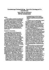
Figure 1: Comparison between the normalized results of first model and split electricity bill. 5000 4000
First of all, as mentioned, the truthfulness degree was not very good concerning the control of room temperature (unprotected thermostat) and concerning the air supply temperature which was manually adjusted.
Base
•
x 10
4
15
Cooling
Table 1: Cumulative errors Temp. [oC] Elec. Heating 0 0.8041 5 0.5619 10 0.3684 15 0.2082 18 0.1395 20 0.1076 24 0.0778
4
6
3000 2000 1000 0 1
2
3
4
5
6
1
2
3
4
5
6
7
8
9
10
11
12
7 8 Month
9
10
11
12
8000
Secondly, electrical plinths are used as the perimeter heating without the appropriate control sequence to avoid simultaneous heating and cold air supply. Furthermore, the building manager has confirmed that the electrical plinths were often on during the summer.
Given that the choice of these balance point temperatures has an impact on the normalization of the simulated results, it is to be noted that this choice was only possible thanks to the originality of the proposed process. Normally, without the application of our method, typical temperatures between 10 and 18 oC and between 12 and 20 oC would have to be fixed and used respectively for heating and cooling degree-days. Steps # 5 and 6 The figures #1 and 2 show the comparison between the normalized simulation results of the first model and the split electricity and gas bill. The relative error related to annual electricity and gas consumption is 28.96 and 48 % respectively. Even if the error regarding the electricity is not neglectable,
6000 Heating
•
4000 2000 0
Figure 2: Comparison between the normalized results of first model and split gas bill. Step # 7 Modification consists in reducing DHW demand so that the basic consumption during summer time would be comparable to the gas bill for the same period. Second simulation Step #2 The balance point temperature for heating degreedays (electrical portion): 24 oC The balance point temperature for cooling degreedays: 10 oC The balance point temperature for heating degreedays (gas portion): 15 oC
- 364 -
Steps # 5 and 6 The balance point temperature for cooling and heating degree-days (electrical portion) did not change because the modification only concerned gas consumption. The figures #3 and 4 show the comparison between the normalized simulation results of the second model and the split electricity and gas bill. The relative error for electricity did not change, but for gas, it has increased up to 95.57%. It is to be noted, however, that the gas consumption is insufficient in winter, while the consumption of electricity is too high. The modification of the model should focus on this problem.
coils) and at decreasing electricity consumption (electrical plinths) during the winter. During the cooling period, it aims at decreasing the electricity consumption of the chiller and the electrical plinths. Third simulation Step #2 The balance point temperature for heating degreedays (electrical portion): 24 oC The balance point temperature for cooling degreedays: 10 oC The balance point temperature for heating degreedays (gas portion): 10 oC
4
Base
6
x 10
Steps # 5 and 6 The figures #5 and 6 show the comparison between the normalized simulation results of the third model and the split electricity and gas bill. We can see an important improvement regarding both the gas and electricity consumption. The relative error related to electricity and gas annual consumption is 9.2 and 2.27 % respectively. Even if the objective for annual electricity consumption is met, the model calibration requires an improvement in the monthly energy consumption.
4 2 0
Heating
15
41
2
3
4
5
6
7
8
9
10
11
12
41
2
3
4
5
6
7
8
9
10
11
12
1
2
3
4
5
6
7 8 Month
9
10
11
12
x 10
10 5 0
Cooling
4
x 10
2
0 4
6 Base
Figure 3: Comparison between the normalized results of second model and split electricity bill.
x 10
4 2 0
600 Heating
6
Base
400
200
41
2
3
4
5
6
7
8
9
10
11
12
41
2
3
4
5
6
7
8
9
10
11
12
1
2
3
4
5
6
7 8 Month
9
10
11
12
x 10
4 2 0 3
0 2
3
4
5
6
7
8
9
10
11
12 Cooling
1 15000
x 10
2 1
Heating
0 10000
Figure 5: Comparison between the normalized results of third model and split electricity bill.
5000
0 1
2
3
4
5
6
7 8 Month
9
10
11
12 600
Figure 4: Comparison between the normalized results of second model and split gas bill. Base
400
Step # 7 As mentioned, the truthfulness degree was not very good concerning the control point of room temperature and the air supply temperature which was manually adjusted. The following modification is proposed: •
The air supply temperature will be established to 15.8 and 18 oC in winter and summer time, respectively, rather than having it vary with the exterior air temperature. This modification aims at increasing gas consumption (heating central
200
0 1
2
3
4
5
6
1
2
3
4
5
6
7
8
9
10
11
12
7 8 Month
9
10
11
12
Heating
15000
10000
5000
0
Figure 6: Comparison between the normalized results of third model and split gas bill.
- 365 -
600
Step # 7 Again, referring to the truthfulness degree of certain data collected, the following modifications are proposed:
Base
400
200
0
•
The rooms temperature set point is increased to 25 oC during the cooling period and it varies between 22.9 and 24 oC during the winter. The purpose of this modification is to increase the energy consumed by the electrical plinths during heating period and to moderate this consumption during cooling period. As already mentioned, the boiler is available from November 1st to May 15, although these dates may not be accurate. To improve the calibration of the gas consumption model in November, the boilers will only be put in operation on November 15.
Fourth simulation Step #2 The balance point temperature for heating degreedays (electrical portion): 24 oC The balance point temperature for cooling degreedays: 10 oC The balance point temperature for heating degreedays (gas portion): 10 oC Steps # 5 and 6 The figures #7 and 8 show the comparison between the normalized simulation results of the fourth model and the split electricity and gas bill. The relative error concerning the annual electricity consumption is 0.46 %; for the monthly electrical consumption, it varies between 0.29% in October and 8.69% in November. The error related to annual gas consumption is also acceptable since it is 3.47%, while the error concerning the monthly gas consumption varies too much and is particularly unacceptable for November.
1
2
3
4
5
6
7
8
9
10
11
12
7 8 Month
9
10
11
12
•
Wait until November 25 to turn on the gas boiler. According to the information given by the building manager, such a thing has already been done in the past, and it was noted that the heating terminal coils could produce enough heat.
•
The set point of air supply temperature varies between 15.8 and 16.9 oC in November and December.
Fifth simulation Step #2 The balance point temperature for heating degreedays (electrical portion): 24 oC The balance point temperature for cooling degreedays: 10 oC The balance point temperature for heating degreedays (gas portion): 5 oC Steps # 5 and 6 The figures #9 and 10 show the comparison between the normalized simulation results of the fifth model and the split electricity and gas bill. 4
6 Base
Base
6
Step # 7 The following modifications are proposed:
x 10
x 10
4 2 0
41
x 10
2
3
4
5
6
7
8
9
10
11
12
6 Heating
Heating
5
Figure 8: Comparison between the normalized results of fourth model and split gas bill.
0
4 2
41
2
3
4
5
6
7
8
9
10
11
12
41
2
3
4
5
6
7
8
9
10
11
12
1
2
3
4
5
6
7 8 Month
9
10
11
12
x 10
4 2 0
0 41
x 10
2
3
4
5
6
7
8
9
10
11
12
3 Cooling
Cooling
4
5000
2
3
3
0
4
6
2
10000
4
6
1 15000
Heating
•
2 1
x 10
2 1 0
0 1
2
3
4
5
6
7 8 Month
9
10
11
12
Figure 7: Comparison between the normalized results of fourth model and split electricity bill.
Figure 9: Comparison between the normalized results of fifth model and split electricity bill.
- 366 -
600
Base
400
200
0 1
2
3
4
5
6
1
2
3
4
5
6
7
8
9
10
11
12
7 8 Month
9
10
11
12
Heating
15000
10000
5000
0
Figure 10: Comparison between the normalized results of fifth model and split gas bill. Since it is the last simulation, the relative errors are presented in table # 2.
Total
% 6.1 3.6 5.2 8.7 5.3 5.9 4.0 2.4 3.9 2.0 4.1 9.0
Error( abs.) relative
MWh 93.85 90.17 83.08 72.87 69.25 70.08 86.69 86.11 79.59 74.50 98.39 101.76
Bill (gas)
Error (abs.) relative
MWh 88.47 87.05 87.66 79.82 73.11 74.49 90.30 84.09 76.62 76.02 94.52 93.33
DOE (gas)
Bill (electricity)
1 2 3 4 5 6 7 8 9 10 11 12
DOE (electricity)
Month
Table 2: Relative errors concerning the electricity and gas consumption
m3 m3 % 8298 7309 13.5 10667 11339 5.9 7193 6898 4.3 4780 4148 15.2 1525 1098 38.9 365 331 10.1 477 443 7.7 385 522 26.1 435 574 24.2 452 452 0 1402 919 52.5 10089 12187 17.2
1005.48 1006.34 0.09 46069 46222 0.33
The validation objective was met for the monthly and annual electrical consumption and for annual gas consumption. Even if the curves of the gas bill and the normalized simulation results per month fit very well visually, the errors that occurred require some explanation. Although the errors for september and october seem high, the absolute value of the difference between the bill and the normalized simulation results represents only 140 m3 of gas. Considering the random use of DHW (which represents the only gas consumption during this period), these errors are entirely acceptable.
For the other months showing errors grater than 10%, the absolute value of this difference varies between 427 m3, in May, and 2100 m3, in December. Even for November (error of 52.5%), this value is only 483 m3 of gas. These differences could be explained by the use of the extractor hoods in the research laboratories which has an impact on the heat recovery system efficiency, as it is explained in this paper. The simulation models include the heat recovery system, but with a constant value of efficiency. To reduce these differences, a specific function in DOE2 software had to be used in order to modulate the efficiency of heat recovery according to the schedule of extractor hoods operation. The problem is that the extractor hoods are randomly used, which makes the simulation difficult to realize. In our opinion, the validated model presented in this paper as the fifth simulation is entirely useful to determine the impact of most energy efficiency measures taken in the building.
ACKNOWLEDGENMENTS The work presented here is a part of a collaborative project between GES Technologies inc. and École de technologie supérieure de Montreal. The project was supported by GES Technologies inc. and the general objective of this project was to develop the software Best Building Facility Management.
CONCLUSION The originality of the proposed validation process could be described as follows: The validation process is dynamic because the normalization of the simulation results and the division of the electricity and gas bill are realized by taking into account the balance point temperatures for appropriate degree-days. These temperatures, as it was shown in this paper, could change during the validation process, as opposed to most cases where these temperatures are arbitrary fixed for the whole process. It is to be noted that these temperatures have an important impact on the modifications applied in the validation and consequently on the quality of the validated model. The method used to choose these temperatures is described in this paper. Heating, cooling and basic monthly energy consumption are taken into account in the validation process. This approach allows the user to target specific building or HVAC elements which can be modified during validation. As it was shown in this paper, the proposed process, applied to energy use in a relatively complex building, is quick and efficient. During the data collection we have identified the truthfulness degree of the collected data. This information is very useful in the validation process,
- 367 -
because it allows the user to modify the corresponding elements first. It is to be noted however that this validation process requires a detailed data collection.
REFERENCES DOE-2 Engineers Manual, Lawrence Berkeley Laboratory and Los Alamos National Laboratory, November 1982. Model National Energy Code of Canada for Building – Canada 1997 Energy Efficiency Standards for Residential and NonResidential Building, California Energy Commission, July 1999 Fundamentals, 1997 ASHRAE Handbook, American Society of Heating, Refrigerating and AirConditioning Engineers, Atlanta, 1997. Air-Conditioning Systems Design Manual, Prepared by the ASHRAE 581-RP Project Team Harold G. Lorsch, Principal Investigator, Atlanta, 1993
- 368 -