Journal of Computational and Applied Mathematics 342 (2018) 375–398
Contents lists available at ScienceDirect
Journal of Computational and Applied Mathematics journal homepage: www.elsevier.com/locate/cam
Stress–strength reliability analysis of system with multiple types of components using survival signature Yiming Liu a, *, Yimin Shi a, *, Xuchao Bai a , Bin Liu b a b
Department of Applied Mathematics, Northwestern Polytechnical University, Xi’an, Shaanxi 710072, China Department of Applied Mathematics, Taiyuan University Of Science And Technology, Taiyuan, Shanxi 030024, China
highlights • • • •
Gompertz stress–strength reliability (SSR) of multiple components system is derived. Generalized confidence intervals for SSR with unknown scale parameters are presented. Modified GCIs for SSR under the common stress and different stresses are given. Efficient algorithms for constructing the Modified GCIs are designed.
article
info
Article history: Received 1 January 2018 Received in revised form 5 April 2018 Keywords: Gompertz distribution Generalized pivotal quantity Maximum spacing estimator Stress–strength reliability Multiple types of components Survival signature
a b s t r a c t In this paper, we study the estimation for stress–strength reliability of the system with multiple types of components based on survival signature. In the situation that different types of components are subjected to different types of random stresses, the maximum likelihood estimator, maximum spacing estimator, bootstrap-p confidence interval, two point estimators and generalized confidence interval using generalized pivotal quantity for system stress–strength reliability are derived under the assumption that the stresses and strengths variables follow the Gompertz distributions with common or unequal scale parameters. Additionally, when the stresses and strengths variables follow the Gompertz distributions with unequal scale parameters, a modified generalized confidence interval for the system stress–strength reliability based on the Fisher Z transformation is also proposed. In the situation that the system is subjected to the common stress, the above point estimators and confidence intervals for the system stress–strength reliability are also developed. Monte Carlo simulations are performed to compare the performance of these point estimators and confidence intervals. A real data analysis is presented for an illustration of the findings. © 2018 Elsevier B.V. All rights reserved.
1. Introduction Stress–strength models are of special importance in engineering applications. A technical system or unit may be subjected to randomly occurring environmental stresses such as pressure, temperature, and humidity. The survival of the system heavily depends on its resistance. In the simplest form of the stress–strength model, a failure occurs when the strength (or resistance) of the component drops below the stress. In this case the stress–strength reliability (SSR) R is defined as the probability that the component’s strength is greater than the stress, that is, R = P(X1 > X2 ), where X1 is the
*
Corresponding authors. E-mail addresses:
[email protected] (Y. Liu),
[email protected] (Y. Shi).
https://doi.org/10.1016/j.cam.2018.04.029 0377-0427/© 2018 Elsevier B.V. All rights reserved.
376
Y. Liu et al. / Journal of Computational and Applied Mathematics 342 (2018) 375–398
random strength of the component and X2 is the random stress placed on it. The stress–strength model has been applied in various fields such as engineering, seismology, oceanography, hydrology, economics and medicine; see for example Johnson [1] and Kotz et al. [2]. Eryılmaz [3] studied Multivariate stress–strength model for coherent structures. The SSR for consecutive k-out-of-n: G system was considered by Eryılmaz [4]. Additionally, Eryılmaz [5] developed the SSR for a coherent system. For more extensive and lucid researches on the stress–strength model by Eryılmaz, see [6–8]. Recently, Liu et al. [9] studied the estimation for SSR of a N-M-cold-standby redundancy system based on progressive Type-II censoring sample. The SSR of a standby redundancy system with independent stress and strength based on different probability distributions, viz. Exponential, Gamma and Lindley distributions was studied by Khan and Jan [10]. Estimations of the reliability in multicomponent stress–strength systems were obtained by Kızılaslan and Nadar [11,12] when the underlying distributions were Weibull distribution and Marshall–Olkin bivariate Weibull distribution. Wang et al. [13] developed inferential procedures for the generalized exponential stress–strength model based on generalized pivotal quantity (GPQ). For more details on the stress–strength model in recent years, see [14–19]. The system signature has been found to be useful for comparisons performance and the quantification of the reliability of coherent system. A lucid review of the theory about signature and its application were presented by Samaniego [20]. The main advantage of system signature is that it separates the structure of the system from the failure time distribution of the components. However, when it comes to real world systems with more than one component type, a reliability analysis based on system signature is pretty complex and not feasible. Therefore, the components are generally regarded as of a single type for simplification. In order to overcome the limitations of system signature, Coolen and Coolen-Maturi [21] presented an improved method, which called survival signature, to conduct reliability analysis of systems with multiple types of components. Recently, Eryılmaz [22] presented the usefulness of system survival signature for computing some important reliability indices of repairable systems with common components. Marginal and joint reliability importance based on survival signature was developed by Eryılmaz et al. [23]. Coolen et al. [24–26] dealt with reliability of systems and networks with multiple types of components based on the survival signature. Eryılmaz and Tuncel [27] generalized the survival signature for unrepairable homogeneous multi-state systems. Pakdaman et al. [28] developed the system SSR based on survival signature. Except for that, there is few literature on the survival signature for SSR of multicomponent system, especially the multicomponent system with multiple types of components. The Gompertz distribution was first introduced by Gompertz [29]. The probability density function (PDF) and cumulative distribution function (CDF) of the two-parameter Gompertz distribution are given by f (x) = α ecx e− c (e α
), x > 0
(1.1)
) , x > 0,
(1.2)
cx −1
and F (x) = 1 − e− c (e α
cx −1
respectively, where c > 0, α > 0 are the scale and shape parameters. The Gompertz distribution with parameters c and α will be denoted by G(c , α ). This distribution plays an important role in modeling survival times, human mortality and actuarial tables. It has many applications, particularly in medical and actuarial studies. In addition, the Gompertz distribution is used as a statistical model in reliability. It has been used as a growth model and also used to fit the tumor growth. Applications and more recent surveys of the Gompertz distribution can be found in [30]. Statistical inference for the Gompertz distribution has received the attention of some authors. Jaheen [31] analyzed record statistics from the Gompertz model based on Bayesian method. Some point and interval estimations for the Gompertz distribution can be referenced from [32–34]. El-Gohary et al. [35] proposed a new generalization of the Gompertz distributions and derived some statistical properties of such distribution. Additionally, based on the analysis of some real data sets [36,37], it is founded that the Gompertz distribution can fit lifetime of some products, such as ball bearing and electrical insulation. In the realm that stress and strength variables follow the Gompertz distributions, Saraçoğlu et al. [38,39] studied the maximum likelihood estimator (MLE), uniformly minimum variance unbiased estimator, Bayes estimator, exact confidence interval and asymptotic confidence interval of component SSR based on the assumption that strength and stress variables followed Gompertz distributions with common and known scale parameter. Karam [40] discussed multicomponent system SSR using Gompertz distribution with unknown shape and known scale parameters. However, there is a few research on the SSR of the Gompertz model, which both the shape and scale parameters are unknown. The assumption of common scale parameters may be very restrictive in practice. Hence, it is necessary to consider the inferential methods for the SSR without the assumption of common scale parameters. This paper considers using survival signature to estimate SSR of system with multiple types of components. Based on the assumption that the underlying distributions of the strength and stress variables are the Gompertz distributions, the remainder of this paper is organized as follows. In Section 2, the expressions for SSR of the system, which is subjected different types of stresses and the common stress, are derived based on survival signature. In Section 3, considering different types of stresses, the MLE, maximum spacing (MSP) estimator, bootstrap-p confidence interval (BCI), two point estimators and generalized confidence interval (GCI) based on GPQ for the system SSR with the assumption of common scale parameters are proposed. Additionally, the finite sample properties of these point estimators and confidence intervals are assessed by Monte Carlo simulation. In Section 4, considering different types of stresses, we derive the MLE, MSP estimator, BCI, two point estimators and GCI for the system SSR under unequal scale parameters. On account of the Fisher Z transformation,
Y. Liu et al. / Journal of Computational and Applied Mathematics 342 (2018) 375–398
377
the modified GCI (MGCI) for the system SSR is given. The performance of the proposed methods is also assessed by Monte Carlo simulation in Section 4. In consideration of the common stress placed on the system, the above point estimators and confidence intervals for system SSR are developed in Section 5. Moreover, the finite sample properties of these point estimators and confidence intervals are assessed by Monte Carlo simulation in this section. Furthermore, a real data analysis is presented in Section 6. Finally, we provide some final conclusions in Section 7. 2. SSR for system with multiple types of components 2.1. SSR for system with multiple types of components with different types of random stresses
∑KConsider a system with K ≥ 2 types of m components. There are mk components of type k ∈ {1, 2, . . . , K } and k=1 mk = m. Assume that the random strengths of the same type of component are independent and identically distributed and different types of components are subjected different types of random stresses. Let random variables Xk:1 and Xk:2 , k = 1, 2, . . . , K represent the strength of the kth type component and the stress impacted on it, respectively. Suppose that Xk:1 and Xk:2 are independent. Define the state vector of components s = (s1 , s2 , . . . , sm ) ∈ {0, 1}m with si = 1 if the ith −
component functions and si = 0 if not. The structure function φ : {0, 1}m → {0, 1} is vitally important to establish theory of system reliability. Define φ for all possible s , with φ (s ) = 1 if the system functions and φ (s ) = 0 if the system does not −
−
−
function for state vector s . Throughout this paper, we restrict attention to coherent systems, which means that φ (s ) is not −
−
decreasing in any of the components of s , so system functioning cannot be improved by poor performance of one or more −
components. It is natural to assume that φ (0) = 0 and φ (1) = 1. Components of the same type can be grouped together and −
−
the state vector can be written as s = (s 1 , s 2 , . . . , s K ), where the sub-vector s k = (sk1 , sk2 , . . . , skmk ) represents the states −
−
−
−
−
of the components of type k. And ski = 1, ik = 1, 2, . . . , mk if the ik th component of type k functions and ski = 0 if not. k k According to Coolen [21], the survival signature for such a system is denoted by Φ (q1 , q2 , . . . , qK ), for qk = 0, 1, . . . , mk . And the survival signature is defined as the probability that ) system functions when the precisely qk components of type ( the mk qk
k function, for each k ∈ {1, 2, . . . , K }. Hence, there are
state vectors s k with precisely qk functioning components,
∑m
−
k k which the states of them are equal to 1. Then it is facile to obtain ik=1 sik = qk . Denote Sqk as the set of these state vectors∑ for components of type k. Furthermore, let Sq1 ,q2 ,...,qK denote the set of all state vectors for the whole system for m which i k ski = qk , k = 1, 2, . . . , K . Hence,
ski k
k
k=1
Φ (q1 , q2 , . . . , qK ) =
[ K ( ) ] ∏ m −1 k
k=1
×
qk
( )
∑
φ s . −
(2.1)
s ∈Sq1 ,q2 ,...,qK −
Denote Nk ∈ {0, 1, . . . , mk } as the number of components of type k in the system that meet Xk:1 > Xk:2 . In particular, assume that X1:1 , . . . , XK :1 are independent and X1:2 , . . . , XK :2 are independent, then the system SSR can be expressed as m1 ∑
R=
=
mK ∑
···
( Φ (q1 , q2 , . . . , qK ) P
qK =0
m1 ∑
mK ∑
···
{Nk = qk }
k=1,2,...,K
q1 = 0
q1 = 0
) ⋂
Φ (q1 , q2 , . . . , qK )
qK =0
K ∏
(2.2)
P (Nk = qk ) .
k=1
Suppose that Fk:1 (xk:1 )(fk:1 (xk:1 )) and Fk:2 (xk:2 )(fk:2 (xk:2 )) are the CDFs(PDFs) of Xk:1 and Xk:2 , k = 1.2, . . . , K , respectively. Therefore, Eq. (2.2) can be rewritten as R=
m1 ∑ q1 =0
where Ik =
∫∞ 0
···
mK ∑ qK =0
[ Φ (q1 , q2 , . . . , qK )
) )] K (( ∏ m k
k=1
qk
Ik
,
(2.3)
[1 − Fk:1 (xk:2 )]qk [Fk:1 (xk:2 )]mk −qk dFk:2 (xk:2 ).
2.2. SSR for system with multiple types of components with the common random stress Follow the system described in Section 2.1, it is assumed that the random strengths of the same component type are independent and identically distributed and different types of components are subjected the common random stress. Let random variables Xk:1 , k = 1, 2, . . . , K and X2 represent the strength of the kth type of component and the common random stress imposed on it, respectively. And, suppose that Xk:1 , k = 1, 2, . . . , K and X2 are independent. Suppose that Fk:1 (xk:1 )
378
Y. Liu et al. / Journal of Computational and Applied Mathematics 342 (2018) 375–398
(fk:1 (xk:1 ))and F2 (x2 )(f2 (x2 )) are the CDFs(PDFs) of Xk:1 , k = 1, 2, . . . , K and Xk:2 , respectively. According to Eqs. (2.1) and (2.2), R can be given by m1 ∑
R=
mK ∑
···
q1 =0
[Φ (q1 , q2 , . . . , qK ) I(q1 , q2 , . . . , qK )] ,
(2.4)
qK =0
where I(q1 , q2 , . . . , qK ) =
{( )
∫ ∞ ∏K
mk qk
k=1
0
} [1 − Fk:1 (x2 )]qk [Fk:1 (x2 )]mk −qk dF2 (x2 ).
3. Inference for SSR with common scale parameters of Xk :1 and Xk :2 under different types of random stresses Suppose that Xk:i ∼ G(ck , αk:i ), k = 1, 2, . . . , K , i = 1, 2, and they are independently distributed. Then Ik can be expressed as ∞
∫ Ik =
[
−
e
αk:1 ck
(eck xk:2 −1)
]qk [
1−e
−
αk:1 ck
(eck xk:2 −1)
]mk −qk [
d 1−e
−
αk:2 ck
(eck xk:2 −1)
]
0 1
∫
α
α
q
uk k:1 k [1 − uk ]mk −qk duk k:2
= 0
mk −qk
∑ (m − q ) k k
=
ik
ik =0
(−1)ik
∑ (m − q ) k k ik
ik =0
α
αk:2 uk k:1
(ik +qk )+αk:2 −1
(3.1)
duk
0
mk −qk
=
1
∫
(−1)ik
αk:2 , αk:1 (ik + qk ) + αk:2
where uk = e−(e
)/ck .
ck xk:2 −1
Hence, Eq. (2.3) can be rewritten as R=
m1 ∑
···
q1 =0
mK ∑
⎡
⎛ ) ( ) m∑ K k −qk ( ∏ mk − qk ⎣Φ (q1 , q2 , . . . , qK ) ⎝ mk (−1)ik
qK =0
k=1
qk
ik =0
ik
⎞⎤ αk:2 ⎠⎦ . αk:1 (ik + qk ) + αk:2
(3.2)
3.1. Maximum likelihood estimator Let Xk:i,1 , . . . , Xk:i,nk:i be a random sample from G(ck , αk:i ), k = 1, 2, . . . , K , i = 1, 2. Denote xk:i,1 , . . . , xk:i,nk:i as the corresponding observed values. In the light of Saraçoğlu et al. [39], the log-likelihood function based on the above samples is given as follows,
ℓk (ck , αk:1 , αk:2 ; xk:1,1 , . . . , xk:1,nk:2 , xk:2,1 , . . . , xk:2,nk:2 ) ⎛ ⎞ ⎧ nk:1 nk:2 ⎪ ∑ ∑ ⎪ ⎪ ⎪ nk:1 log αk:1 + nk:2 log αk:2 + ck ⎝ xk:1,i + xk:2,j ⎠ ⎪ ⎪ ⎨ i=1 j=1 ⎞ ⎛ = nk:2 nk:1 ⎪ ⎪ ∑ ∑ ( ) ( ) ⎪ 1 ⎪ − ⎝α ⎪ eck xk:2,j − 1 ⎠ . eck xk:1,i − 1 + αk:2 k:1 ⎪ ⎩ ck i=1
j=1
Hence, it is facile to obtain MLEs of αk:1 and αk:2 ,
αˆ k:1 =
αˆ k:2 =
nk:1 cˆk−1
∑nk:1 (
−1
∑nk:2 (
i=1
nk:2 cˆk
j=1
),
(3.3)
).
(3.4)
ecˆk xk:1,i − 1
ecˆk xk:2,j − 1
The MLE cˆk of ck is the solution of the following nonlinear equation
(wk:1 + wk:2 ) − (hk:1 (ck ) + hk:2 (ck )) +
(nk:1 + nk:2 ) ck
= 0,
Y. Liu et al. / Journal of Computational and Applied Mathematics 342 (2018) 375–398
379
∑nk:1 ∑nk:2 ∑nk:1 ∑n ck xk:1,i where wk:1 = / i=k:11 (eck xk:1,i − 1) and hk:2 (ck ) = i= 1 xk:1,i , wk:2 = j=1 xk:2,j , hk:1 (ck ) = nk:1 i=1 xk:1,i e ∑nk:2 ∑ n nk:2 j=1 xk:2,j eck xk:2,j / j=k:12 (eck xk:2,j − 1) . Therefore, cˆk can be obtained as a solution of the nonlinear equation of the form ck = H(ck ),
(3.5)
where H(ck ) = (nk:1 + nk:2 )/(hk:1 (ck ) + hk:2 (ck ) −wk:1 −wk:2 ) . Then, cˆk is a fixed point solution of the nonlinear equation (3.5), its value can be obtained by using Newton iteration method. When we obtain cˆk , the MLEs of αk:i , k = 1, . . . , K , i = 1, 2, can be obtained from Eqs. (3.3) and (3.4). Hence, the MLE of R obtained from Eq. (3.2) by using the invariance property of MLE is expressed as, Rˆ 1 =
m1 ∑
···
q1 = 0
mK ∑
⎡
⎛ ( ) m∑ ) K k −qk ( ∏ mk − qk ⎣Φ (q1 , q2 , . . . , qK ) ⎝ mk (−1)ik
qK =0
qk
k=1
ik
ik =0
⎞⎤ αˆ k:2 ⎠⎦ . αˆ k:1 (ik + qk ) + αˆ k:2
(3.6)
3.2. Maximum spacing estimator The MSP method was introduced by Cheng and Amin [41] as an alternative to the MLE method. Ranneby [42] derived the MSP method from an approximation of the Kullback–Leibler divergence (KLD). Ekström [43] showed that the MSP estimators have better properties than MLE for small samples. MSP estimator has all the nice properties of MLE such as consistency, asymptotic normality, efficiency and invariance under one-to-one transformations. For a detailed survey of the MSP method, the reader is referred to [41–44]. Denote X1 , X2 , . . . , Xn as a random sample from a population with true (but unknown) CDF F (x) and PDF f (x). Let X = (X(1) , X(2) , . . . , X(n) ) be the corresponding order statistics. It is supposed that the sample X1 , X2 , . . . , Xn from the population with CDF {Fθ (x, θ ); θ ∈ Θ } and PDF {fθ (x, θ ); θ ∈ Θ }, where θ is an unknown k-dimensional (k ≥ 1) parameter vector and Θ ∈ Rk . In addition, suppose that F (x) and {Fθ (x, θ ); θ ∈ Θ } are continuous CDFs with the same support. The KLD between F (x) and Fθ (x, θ ) is given by
⏐ ⏐ ⏐ f (x) ⏐ ⏐ dx. fθ (x, θ ) ⏐
∫
D(F , Fθ ) =
f (x) log ⏐⏐
The KLD can be approximated by estimating D(F , Fθ ) with n 1∑
n
i=1
⏐ ⏐ ⏐ f (xi ) ⏐ ⏐. fθ (xi , θ ) ⏐
log ⏐⏐
(3.7)
Minimizing quantity (3.7) with respect to θ, the estimator of θ can be found, which is actually the well-known MLE. It should be noted that for some continuous distribution, log f (xi ), i = 1, 2, . . ., n, may not be bounded from above. According to Ranneby [42], another approximation of the KLD is given by n+1 ∑
1 n+1
i=1
⏐ ⏐
log ⏐⏐
⏐ ⏐ ⏐, Fθ (x(i) , θ ) − Fθ (x(i−1) , θ ) ⏐ F (x(i) ) − F (x(i−1) )
(3.8)
where Fθ (x(0) , θ ) ≡ 0, Fθ (x(n+1) , θ ) ≡ 1 and x = (x(1) , x(2) , . . . , x(n) ) is the observed value of X = (X(1) , X(2) , . . . , X(n) ). By minimizing quantity (3.8), the MSP estimator of θ is obtained. Minimizing quantity (3.8) is equivalent to maximizing: n+1 ∑
M(θ ) =
log[Fθ (x(i) , θ ) − Fθ (x(i−1) , θ )].
(3.9)
i=1
Therefore, the MSP estimator can be obtained by maximizing M(θ ) with respect to θ. Denote Xk:i = (Xk:i,(1) , . . . , Xk:i,(nk:i ) ), k = 1, 2, . . . , K , i = 1, 2, as the corresponding order statistics of Xk:i,1 , . . . , Xk:i,nk:i . Let xk:i = (xk:i,(1) , . . . , xk:i,(nk:i ) ) be the observed value of Xk:i = (Xk:i,(1) , . . . , Xk:i,(nk:i ) ). On the basis of the MSP method, we have M(ck , αk:1 , αk:2 ) nk:1 +1
=
∑
nk:2 +1
j1 =1
=
[
]
log Fk:1 (xk:1,(j1 ) ) − Fk:1 (xk:1,(j1 −1) ) +
∑
[
log Fk:2 (xk:2,(j2 ) ) − Fk:2 (xk:2,(j2 −1) )
j2 =1
⎧ n +1 [ α (cx ) ( c x )] k:1 α ∑ ⎪ − ck:1 e k k:1,(j1 −1) −1 − ck:1 e k k:1,(j1 ) −1 ⎪ ⎪ k k log e − e + ⎪ ⎪ ⎨ j =1 1
[ α (cx ) ( c x )] nk:2 +1 ⎪ α ∑ ⎪ − ck:2 e k k:2,(j2 −1) −1 − ck:2 e k k:2,(j2 ) −1 ⎪ ⎪ k k log e − e , k = 1, . . . , K , ⎪ ⎩ j2 =1
]
380
Y. Liu et al. / Journal of Computational and Applied Mathematics 342 (2018) 375–398
where xk:1,(0) = xk:2,(0) = 0 and xk:1,(nk:1 +1) = xk:2,(nk:2 +1) = +∞. Then, the partial derivatives of M(ck , αk:1 , αk:2 ) with respect to ck , αk:1 and αk:2 can be respectively given by
∂ M(ck , αk:1 , αk:2 ) ∂ ck 2 nk:i +1 ∑ ∑ (1 − ck xk:i,(j −1) )fk:i (xk:i,(j −1) ) − (1 − ck xk:i,(j ) )fk:i (xk:i,(j ) ) − αk:i (Fk:i (xk:i,(j ) ) − Fk:i (xk:i,(j −1) )) i i i i i i [ ] = , ck2 Fk:i (xk:i,(ji ) ) − Fk:i (xk:i,(ji −1) ) i=1 j =1 i
∂ M(ck , αk:1 , αk:2 ) ∂αk:1 nk:1 +1 ∑ fk:1 (xk:1,(j ) ) − fk:1 (xk:1,(j −1) ) + αk:1 (Fk:1 (xk:1,(j ) ) − Fk:1 (xk:1,(j −1) )) 1 1 1 [ 1 ] = , ck Fk:1 (xk:1,(j1 ) ) − Fk:1 (xk:1,(j1 −1) ) j =1 1
∂ M(ck , αk:1 , αk:2 ) ∂αk:2 nk:2 +1 ∑ fk:2 (xk:2,(j ) ) − fk:2 (xk:2,(j −1) ) + αk:2 (Fk:2 (xk:2,(j ) ) − Fk:2 (xk:2,(j −1) )) 2 2 2 [ 2 ] = . ck Fk:2 (xk:2,(j2 ) ) − Fk:2 (xk:2,(j2 −1) ) j =1 2
The MSP estimators of parameters ck , αk:1 and αk:2 , which are denoted by c˜k , α˜ k:1 and α˜ k:2 , respectively, can be obtained by the following nonlinear equations
⎧ ∂ M(ck , αk:1 , αk:2 ) ⎪ ⎪ =0 ⎪ ⎪ ∂ ck ⎪ ⎪ ⎨ ∂ M(c , α , α ) k k:1 k:2 =0 ⎪ ∂α k:1 ⎪ ⎪ ⎪ ∂ M(ck , αk:1 , αk:2 ) ⎪ ⎪ ⎩ = 0. ∂αk:2
(3.10)
It should be noted that, in general, there is no close form for the solution of the nonlinear equations (3.10). Hence, numerical methods need to be applied in order to find the corresponding parameter estimators. Hence, the MSP estimator of R can be given by Rˆ 2 =
m1 ∑
···
q1 =0
mK ∑
⎡
⎛ ) ( ) m∑ K k −qk ( ∏ mk − qk ⎣Φ (q1 , q2 , . . . , qK ) ⎝ mk (−1)ik
qK =0
k=1
qk
ik =0
ik
⎞⎤ α˜ k:2 ⎠⎦ . α˜ k:1 (ik + qk ) + α˜ k:2
(3.11)
3.3. Generalized confidence interval and two point estimators base on generalized pivotal quantity To derive GCI and two point estimators of R, the following Lemma 3.1 (see [13]) and Theorem 3.2 are needed. Lemma 3.1. Let Z1 , . . . , Zn be a random sample from the exponential distribution with mean θ and Z(1) < Z(2) < · · · < Z(n) be the corresponding order statistics. Furthermore, let Si =
i ∑
Z(j) + (n − i)Z(i) , i = 1, . . . , n,
j=1
T =2
n−1 ∑
log(Sn /Si ).
i=1
Then (1) T and Sn are independent; (2) T ∼ χ 2 (2n − 2) and 2Sn /θ ∼ χ 2 (2n). Theorem 3.2. Let f (c) =
ebc − 1 eac − 1
,
where b > a > 0 are constants. Then (1) f (c) is strictly increasing on (0, +∞); (2) lim f (c) = ba . c →0+
Y. Liu et al. / Journal of Computational and Applied Mathematics 342 (2018) 375–398
381
Proof. (1) Let f ′ (c) be the derivative of f (c) with respect to c , then df (c)
f ′ (c) =
=
dc
(b − a)e(b+a)c − (bebc − aeac ) (eac − 1)2
.
Denote g(c) = (b − a)e(b+a)c /(bebc − aeac ) and let g ′ (c) be the derivative of g(c) with respect to c , hence g ′ (c) =
dg(c) dc
ab(b − a)e(b+a)c (ebc − eac )
=
(bebc − aeac )2
.
On the basis of the condition that b > a > 0 are constants, g ′ (c) is strictly greater than zero on (0, +∞). Therefore, g(c) is strictly increasing on (0, +∞) and g(c) > g(0) = 1. Then, f ′ (c) is strictly greater than zero on (0, +∞) and f (c) is strictly increasing on (0, +∞). (2) According to the L’Hospital’s rule, lim f (c) = lim
c →0+
d(ebc − 1)/dc
c →0+
bebc
= lim
− 1)/dc
d(eac
aeac
c →0+
=
b a
.
Denote Xk:i = (Xk:i,(1) , . . . , Xk:i,(nk:i ) ), k = 1, 2, . . . , K , i = 1, 2, as the corresponding order statistics of Xk:i,1 , . . . ,
( ( c X )) α − k:i e k k:i,(nk:i ) −1 , . . . , 1 − e ck are the order statistics from the standard ( cX ) uniform distribution U(0, 1) with sample size nk:i . Thus Zk:i,(j) = e k k:i,(j) − 1 /ck , j = 1, 2, . . . , nk:i , are the order statistics from the exponential distribution with mean 1/αk:i and sample size nk:i . (
−
Xk:i,nk:i . As a consequence, 1 − e
αk:i ck
(
))
c X e k k:i:(1) −1
Define Tk (ck ) = 2
2 nk:i −1 ∑ ∑ i=1
log(Sk:i,nk:i /Sk:i,l ),
(3.12)
l=1
∑l
where Sk:i,l = j=1 Zk:i,(j) + (nk:i − l)Zk:i,(l) , k = 1, 2, . . . , K , i = 1, 2, l = 1, 2, . . . , nk:i . According to Lemma 3.1, we have Tk (ck ) ∼ χ 2 (2nk:1 + 2nk:2 − 4). It is noticed that Sk:i,nk:i Sk:i,l
=1+
Sk:i,nk:i − Sk:i,l Sk:i,l Zk:i,(l+1)
=1+
Zk:i,(l) Zk:i,(1) Zk:i,(l)
+ ··· +
+ ··· +
Zk:i,(n
k:i ) Zk:i,(l)
Zk:i,(l−1) Zk:i,(l)
− (nk:i − l)
+ (nk:i − l + 1)
.
According to Theorem 3.2, it is easy to reach that Tk (ck ) is strictly increasing on (0, +∞), and lim Tk (ck ) = 2
ck →0+
2 nk:i −1 ∑ ∑ i=1
log(Wk:i,nk:i /Wk:i,l ),
l=1
lim Tk (ck ) = +∞,
ck →+∞
∑2 ∑n
∑l
−1
k:i log(Wk:i,nk:i /Wk:i,l ). Therefore, Tk (ck ) follow left truncated where Wk:i,l = l=1 j=1 Xk:i,(j) + (nk:i − l)Xk:i,(l) . Let Wk = 2 i=1 2 chi square distribution, denoted by LT χ (2nk:1 + 2nk:2 − 4, Wk ) with degree of freedom 2nk:1 + 2nk:2 − 4 and Tk (ck ) > Wk . Let Tk ∼ LT χ 2 (2nk:1 + 2nk:2 − 4, Wk ) and T ′ k ∼ χ 2 (2nk:1 + 2nk:2 − 4), then the CDF FTk of Tk can be given by
FT ′ k (tk ) − FT ′ k (Wk )
FTk (tk ) =
1 − FT ′ k (Wk )
,
where FT ′ k is the CDF of T ′ k . For a given Tk ∼ LT χ 2 (2nk:1 + 2nk:2 − 4, Wk ), the equation Tk (ck ) = Tk has the unique solution which is denoted by ck = gk (Tk , Xk:1 , Xk:2 ). The solution of the equation Tk (ck ) = Tk can be obtained by the bisection method. Notice that Uk:i = 2αk:i Sk:i,nk:i ∼ χ 2 (2nk:i ), k = 1, . . . , K , i = 1, 2, then αk:i = Uk:i /(2Sk:i,nk:i ). Using the substitution method proposed by Weerahandi [45], we obtain the following GPQ,
WR =
⎡ ⎛ ⎧ ( ) m∑ ) m1 mK K k −qk ( ⎪ ∑ ∑ ∏ ⎪ mk mk − qk ⎪ ⎣ ⎝ ⎪ · · · Φ q , q , . . . , q (−1)ik × ( ) 1 2 K ⎨ qk ik q1 = 0
qK =0
where sk:i,nk:i =
k=1
ik =0
Uk:2 /(2sk:2,nk:2 )
⎪ ⎪ ⎪ ⎪ ⎩
)]
Uk:1 /(2sk:1,nk:1 ) (ik + qk ) + Uk:2 /(2sk:2,nk:2 ) egk (Tk ,xk:1 ,xk:2 )xk:i,(j) − 1 /gk (Tk , xk:1 , xk:2 )
∑nk:i [( j=1
)
]
(3.13)
,
and xk:i = (xk:i,(1) , . . . , xk:i,(nk:i ) ) is the observed value of
Xk:i = (Xk:i,(1) , . . . , Xk:i,(nk:i ) ). Denote WR,β as the β percentile of WR , then [WR,β/2 , WR,(1−β )/2 ] is a 1 − β GCI for R. And WR,β is a 1 − β generalized confidence lower limit (GCLL) for R. The value of WR,β can be obtained by using the following algorithm.
382
Y. Liu et al. / Journal of Computational and Applied Mathematics 342 (2018) 375–398
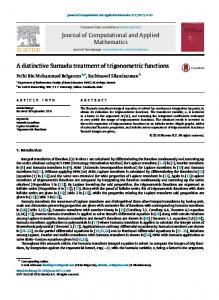
Fig. 1. Compound system with two types components.
Algorithm 1. GCI and GCLL for R with common scale parameters of Xk:i under different types of random stresses. (1) Generate a realization tk of Tk from LT χ 2 (2nk:1 + 2nk:2 − 4, Wk ), k = 1, . . . , K . Then for given samples Xk:1 , Xk:2 , obtain a realization gk of gk (Tk , Xk:1 , Xk:2 ) from equation Tk (ck ) = tk . (2) Generate a realization of Uk:i from χ 2 (2nk:i ), i = 1, 2. Then compute WR on the basis of Eq. (3.13). (3) Repeat the steps (1) and (2) N times. Then there are N values of WR . (4) Arrange all WR values in ascending order: WR,(1) < WR,(2) < · · · < WR,(N) . Then a 1 − β GCI and GCLL for R can be given by [WR,(N β/2) , WR,(N −N β/2 ) ] and WR,β N , respectively. In addition, based on WR,(1) , WR,(2) , . . . , WR,(N) , the following two point estimators for R are proposed. One is given by Rˆ 3 =
N 1 ∑
N
WR,(s) ,
(3.14)
s=1
and the other, which is based on Fisher Z transformation Ys = log[(1 + WR,(s) )/(1 − WR,(s) ) ], s = 1, 2, . . ., N , is given by ¯
Rˆ 4 = where Y¯ =
eY − 1 eY¯ + 1
∑N
,
s=1 Ys
(3.15)
/N .
3.4. Bootstrap-p confidence interval This subsection uses bootstrap-p method, which was proposed by Efron [46], to obtain BCI and bootstrap-p confidence lower limit (BCLL). On the basis of Kundu and Gupta [47], the following procedures are presented to estimate the BCI of R. Bootstrap-p Confidence Interval Step 1: According to the observed value {xk:i,1 , xk:i,2 , . . . , xk:i,nk:i } of sample {Xk:i,1 , Xk:i,2 , . . . , Xk:i,nk:i }, k = 1, . . . , K , i = 1, 2, compute cˆk , αˆ k:1 and αˆ k:2 . Step 2: Using cˆk and αˆ k:1 generate a bootstrap sample value {x∗k:1,1 , x∗k:1,2 , . . . , x∗k:1,n } and similarly using cˆk and αˆ k:2 k:1 generate a bootstrap sample value {x∗k:2,1 , x∗k:2,2 , . . . , x∗k:2,n }. Based on these sample values, compute the bootstrap estimator of R using Eqs. (3.3)–(3.6), denoted by Rˆ ∗1 . Step 3: Repeat Step 2 N times. Then there are N values of Rˆ ∗1 .
k:2
[
]
Step 4: Arrange all Rˆ ∗1 values in ascending order: Rˆ ∗1,(1) < Rˆ ∗1,(2) < · · · < Rˆ ∗1,(N) . Then Rˆ ∗1,(β N /2 ) , Rˆ ∗1,((N −γ N)/2 ) is a 1 − β BCI for R. And Rˆ ∗1,β N is a 1 − β BCLL for R. 3.5. Simulation study In this subsection, a Monte Carlo simulation study is conducted to assess the finite sample properties of the proposed estimation methods for R with MATLAB software tool. Consider the compound system in Fig. 1, which has two types of components and each type has two common components. Then the survival signature of the system is presented in Table 1. Based on the system in Fig. 1, the proposed four different point estimators are compared with each other in terms of bias and mean square error (MSE). Due to people are more interested in the confidence lower limit (CLL) for R in practice, the proposed GCI and BCI for R are compared in terms of coverage percentage (CP) and average CLL. Notice that the CDF of the GPQ WR does not depend on the scale parameters c1 and c2 . Hence, without loss of generality, fix c2 = 2c1 , α2:i = 2α1:i , n2:i = n1:i = ni , i = 1, 2, and α1:1 = c1 = 1 in the simulation study. The values of shape parameter α1:2 are considered for 3, 7, 12 and 19, respectively. Then the corresponding values of shape parameter α2:2 are 6, 14, 24 and 38, respectively. The sample sizes (n1 , n2 ) are considered for (10, 10), (10, 15), (15, 10) and (15, 15), respectively. The
Y. Liu et al. / Journal of Computational and Applied Mathematics 342 (2018) 375–398
383
Table 1 Survival signature of the system in Fig. 1. l1
l2
Φ (l1 , l2 )
l1
l2
Φ (l1 , l2 )
l1
l2
Φ (l1 , l2 )
0 0 0
0 1 2
0 0 0
1 1 1
0 1 2
0 0 1 /2
2 2 2
0 1 2
0 1 /2 1
Table 2 The biases and MSEs of the 4 different estimators for R (common scale parameters). (α1:1 , α1:2 , c1 )
(n1 , n2 )
R
Rˆ 1 Bias
MSE
Bias
MSE
Bias
MSE
Bias
MSE
(1, 3, 1)
(10, 10) (10, 15) (15, 10) (15, 15)
0.5400
0.0242 0.0210 0.0199 0.0190
0.0131 0.0112 0.0097 0.0084
−0.0127 −0.0120 −0.0152 −0.0102
0.0031 0.0031 0.0029 0.0027
0.0164 0.0125 0.0102 0.0130
0.0108 0.0096 0.0078 0.0071
0.0257 0.0203 0.0176 0.0193
0.0118 0.0103 0.0083 0.0076
(1, 7, 1)
(10, 10) (10, 15) (15, 10) (15, 15)
0.7562
0.0215 0.0212 0.0184 0.0149
0.0069 0.0062 0.0050 0.0045
−0.0126 −0.0146 −0.0105 −0.0102
0.0017 0.0019 0.0016 0.0015
0.0105 0.0147 0.0039 0.0107
0.0053 0.0048 0.0043 0.0041
0.0230 0.0259 0.0139 0.0193
0.0058 0.0054 0.0045 0.0044
(1, 12, 1)
(10, 10) (10, 15) (15, 10) (15, 15)
0.8477
0.0143 0.0145 0.0109 0.0105
0.0033 0.0031 0.0024 0.0023
−0.0112 −0.0089 −0.0098 −0.0089
0.0010 0.0008 0.0007 0.0007
0.0077 0.0118 0.0025 0.0063
0.0026 0.0024 0.0021 0.0018
0.0187 0.0218 0.0112 0.0140
0.0028 0.0027 0.0021 0.0019
(1, 19, 1)
(10, 10) (10, 15) (15, 10) (15, 15)
0.9005
0.0092 0.0087 0.0061 0.0066
0.0016 0.0015 0.0012 0.0011
−0.0077 −0.0081 −0.0070 −0.0077
0.0004 0.0004 0.0004 0.0004
0.0078 0.0096 0.0004 0.0056
0.0012 0.0012 0.0010 0.0008
0.0165 0.0175 0.0073 0.0117
0.0014 0.0013 0.0010 0.0009
Rˆ 2
Rˆ 3
Rˆ 4
Table 3 The CPs and average CLLs of GCI and BCI for R based on confidence level 0.9 and 0.95 (common scale parameters). (α1:1 , α1:2 , c1 )
(n1 , n2 )
R
GCI (0.9)
GCI (0.95)
BCI (0.9)
BCI (0.95)
CP
GCLL
CP
GCLL
CP
BCLL
CP
BCLL
(1, 3, 1)
(10, 10) (10, 15) (15, 10) (15, 15)
0.5400
0.8722 0.8820 0.8844 0.8894
0.4218 0.4292 0.4265 0.4413
0.9420 0.9368 0.9542 0.9422
0.3830 0.3959 0.3902 0.4090
0.7862 0.7780 0.7860 0.7784
0.4428 0.4464 0.4593 0.4672
0.8640 0.8508 0.8648 0.8562
0.4089 0.4095 0.4249 0.4355
(1, 7, 1)
(10, 10) (10, 15) (15, 10) (15, 15)
0.7562
0.8756 0.8688 0.8792 0.8580
0.6582 0.6752 0.6613 0.6776
0.9424 0.9440 0.9468 0.9356
0.6202 0.6365 0.6268 0.6474
0.7336 0.7346 0.7468 0.7362
0.6984 0.6996 0.7012 0.7046
0.8360 0.8220 0.8384 0.8368
0.6635 0.6672 0.6716 0.6773
(1, 12, 1)
(10, 10) (10, 15) (15, 10) (15, 15)
0.8477
0.8606 0.8340 0.8792 0.8758
0.7761 0.7861 0.7785 0.7882
0.9350 0.9240 0.9474 0.9536
0.7459 0.7592 0.7514 0.7644
0.7280 0.7344 0.7362 0.7262
0.8042 0.8105 0.8086 0.8139
0.8266 0.8186 0.8206 0.8340
0.7776 0.7861 0.7860 0.7936
(1, 19, 1)
(10, 10) (10, 15) (15, 10) (15, 15)
0.9005
0.8323 0.8458 0.9066 0.8728
0.8501 0.8582 0.8561 0.8596
0.9186 0.9280 0.9602 0.9488
0.8305 0.8382 0.8383 0.8420
0.6868 0.7344 0.7294 0.7260
0.8722 0.8697 0.8697 0.8711
0.7888 0.8124 0.8160 0.8324
0.8508 0.8512 0.8529 0.8557
confidence level considers β = 0.9 and β = 0.95. After that, we report the results based on 5000 replications in Tables 2 and 3. It is observed from Table 2 that the relationship among MLE Rˆ 1 , MSP estimator Rˆ 2 , and two different point estimators based on GPQ Rˆ 3 , Rˆ 4 in terms of MSEs is Rˆ 2 < Rˆ 3 < Rˆ 4 < Rˆ 1 . The point estimator Rˆ 3 is always superior to Rˆ 1 and Rˆ 4 with respect to biases and MSEs, and its biases have the best performance among these four point estimators when (n1 , n2 ) = (15, 10). However, both the biases and MSEs of Rˆ 2 are superior to the other three point estimators when (n1 , n2 ) = (10, 15). In most cases, Rˆ 2 has the underestimation for R, while the other three point estimators have the overestimation for R. In addition, for fixed n1 and n2 , MSEs of the four different point estimators decrease as αk:2 , k = 1, 2, increase. Especially, both the biases and MSEs of these point estimators decrease as αk:2 increase when R ≥ 0.7562. For fixed αk:2 and n1 , the larger the value of n2 , the smaller the MSEs of all the four different estimators. Similarly, for fixed αk:2 and n2 , the larger the value of n1 , the smaller the MSEs of all the four different estimators. From the above we can find that MSP estimator Rˆ 2 has the best performance in terms of MSEs.
384
Y. Liu et al. / Journal of Computational and Applied Mathematics 342 (2018) 375–398
It is clear from Table 3 that CPs of the proposed GCI for R are quite close to the confidence level, but the deviations between the CPs of BCI and confidence level are relatively large. GCLLs are always smaller than BCLLs at the same confidence level. Moreover, for fixed n1 and n2 , the CPs of BCI decrease as αk:2 , k = 1, 2, increase. For fixed αk:2 and n1 , the larger the value of n2 , the larger the GCLLs and BCLLs. Similarly, for fixed αk:2 and n2 , the larger the value of n1 , the larger the GCLLs and BCLLs. These findings show that the performance of the proposed GCI for R is very satisfactory for all cases. 4. Inference for SSR with unequal scale parameters of Xk :1 and Xk :2 under different types of random stresses Suppose that Xk:i ∼ G(ck:i , αk:i ), k = 1, 2, . . . , K , i = 1, 2, and they are independently distributed. Then Ik can be expressed as ∞
∫ Ik =
[
α
− c k:1 (eck:1 xk:2 −1)
e
k:1
] qk [
0 mk −qk
∑ (m − q ) k k
=
ik
ik =0
(−1)
ik
∑ (m − q ) k k ik
ik =0
∑ (m − q ) k k ik
ik =0
∞
∫
(−1)
ik
αk:2 e
∫
−
(
αk:1 ik +qk ck:1
[
∞
αk:2 /ck:2 [
αk:2 e
(
αk:1 ik +qk
mk −qk
=
k:1
α
]mk −qk [
d 1−e
) (eck:1 xk:2 −1)
− c k:2 (eck:2 xk:2 −1)
eck:2 xk:2 e
k:2
]
α
− c k:2 (eck:2 xk:2 −1) k:2
dxk:2
0
mk −qk
=
α
− c k:1 (eck:1 xk:2 −1)
1−e
(−1) e ik
ck:1
(
)
αk:1 ik +qk α + c k:2 ck:1 k:2
] ) + αk:2 ∫
∞
ck:2
e
−
] −
e
(
)
)c /c αk:1 ik +qk ( ck:2 k:1 k:2 ck:1 αk:2 uk
(
)
) c /c αk:1 ik +qk ( ck:2 k:1 k:2 ck:1 αk:2 uk
αk:2 /ck:2
ck:2
αk:2
uk e−uk
1 ck:2 uk
duk
e−uk duk ,
where uk = αk:2 eck:2 xk:2 /ck:2 . Define [
mk −qk
Ak =
∑ (m − q ) k k ik
ik =0
(−1) e ik
(
αk:1 ik +qk ck:1
) + αk:2 ck:2
]
.
Consider that e−uk =
∞ ∑ (−1)l ul
k
l=0
e
−
(
)
l!
,
) c /c αk:1 ik +qk ( ck:2 k:1 k:2 ck:1 αk:2 uk
=
∞ ∑ (−1)j [αk:1 (ik + qk ) /ck:1 ]j (ck:2 uk /αk:2 )jck:1 /ck:2 , j! j=0
then
∫ ∞ ∞ ∑ (−1)j [αk:1 (ik + qk ) /ck:1 ]j (ck:2 /αk:2 )jck:1 /ck:2 jc /c Ik = Ak uk k:1 k:2 e−uk duk j! αk:2 /ck:2 j=0 [ ] ∫ αk:2 /ck:2 ∞ j j jc / c ∑ (−1) [αk:1 (ik + qk ) /ck:1 ] (ck:2 /αk:2 ) k:1 k:2 jck:1 jc /c Γ( + 1) − uk k:1 k:2 e−uk duk = Ak j! ck:2 0 j=0 [ ] (4.1) ∞ ∞ ∑ (−1)j [αk:1 (ik + qk ) /ck:1 ]j (ck:2 /αk:2 )jck:1 /ck:2 ∑ (−1)l ∫ αk:2 /ck:2 (jc /c )+l+1 jck:1 k:1 k:2 = Ak Γ( + 1) − uk duk j! ck:2 l! 0 j=0 l=0 [ ] ∞ ∞ ∑ ∑ (−1)l (αk:2 /ck:2 )(jck:1 /ck:2 ) +l+1 (−1)j [αk:1 (ik + qk ) /ck:1 ]j (ck:2 /αk:2 )jck:1 /ck:2 jck:1 = Ak Γ( + 1) − . j! ck:2 l![(jck:1 /ck:2 ) + l + 1] j=0
l=0
4.1. Maximum likelihood estimator Let Xk:i,1 , . . . , Xk:i,nk:i be a random sample from G(ck:i , αk:i ), k = 1, 2, . . . , K , i = 1, 2, and xk:i,1 , . . . , xk:i,nk:i be the corresponding observed values. Then, the log-likelihood function based on the above samples is given as follows,
ℓk:i (ck:i , αk:i ; xk:i,1 , . . . , xk:i,nk:i ) = nk:i log αk:i + ck:i
nk:i ∑ j=1
xk:i,j −
nk:i ( αk:i ∑
ck:i
eck:i xk:i,j − 1 .
j=1
)
Y. Liu et al. / Journal of Computational and Applied Mathematics 342 (2018) 375–398
385
Hence, it is facile to obtain that
αˆ k:i =
nk:i cˆk−:i1
∑nk:i ( j=1
).
(4.2)
ecˆk:i xk:i,j − 1
The MLE cˆk:i of ck:i is the solution of following nonlinear equation
wk:i − hk:i (ck:i ) + nk:i /ck:i = 0, ∑nk:i ∑nk:i ∑n ck:i xk:i,j where wk:i = / j=k:1i (eck:i xk:i,j − 1) . Therefore, cˆk:i can be obtained as a solution j=1 xk:i,j and hk:i (ck:i ) = nk:i j=1 xk:i,j e of the nonlinear equation of the form ck:i = H(ck:i ),
(4.3)
where H(ck:i ) = nk:i /(hk:i (ck:i ) − wk:i ) . Then, cˆk:i is a fixed point solution of the nonlinear equation (4.3), its value can be obtained by using Newton iteration method. When we obtain cˆk:i , the MLEs of αk:i , k = 1, . . . , K , i = 1, 2, are obtained from Eq. (4.2). Hence, the MLE of R is obtained from Eqs. (2.3) and (4.1) by using the invariance property of MLE’s, R˜ 1 =
m1 ∑
mK ∑
···
q1 =0
[
) )] K (( ∏ mk ˆ Φ (q1 , q2 , . . . , qK ) , Ik
qK =0
k=1
(4.4)
qk
where ∞ ∑ (−1)j [αˆ k:1 (ik + qk ) /ˆck:1 ]j (cˆk:2 /αˆ k:2 )jcˆk:1 /ˆck:2 Iˆk = Aˆ k j! j=0
[
mk −qk
Aˆ k =
∑ (m − q ) k k ik
ik =0
(−1) e ik
(
)
αˆ k:1 ik +qk αˆ + cˆ k:2 cˆk:1 k:2
[ Γ(
jcˆk:1 cˆk:2
] ∞ ∑ (−1)l (αˆ k:2 /ˆck:2 )(jcˆk:1 /ˆck:2 ) +l+1 + 1) − , l![(jcˆk:1 /ˆck:2 ) + l + 1] l=0
]
.
4.2. Maximum spacing estimator Denote Xk:i = (Xk:i,(1) , . . . , Xk:i,(nk:i ) ), k = 1, 2, . . . , K , i = 1, 2, as the corresponding order statistics of Xk:i,1 , . . . , Xk:i,nk:i . Let xk:i = (xk:i,(1) , . . . , xk:i,(nk:i ) ) be the observed value of Xk:i = (Xk:i,(1) , . . . , Xk:i,(nk:i ) ). On the basis of the MSP method proposed in Section 3.3, we have M(ck:i , αk:i ) nk:i +1
=
∑
[
log Fk:i (xk:i,(j) ) − Fk:i (xk:i,(j−1) )
]
j=1 nk:i +1
=
∑
[ log e
( ) α c x − c k:i e k:i k:i,(j−1) −1 k:i
( )] α c x − c k:i e k:i k:i,(j) −1
−e
k:i
, k = 1, . . . , K , i = 1, 2,
j=1
where xk:i,(0) = 0 and xk:i,(nk:i +1) = +∞. Then taking partial derivatives of M(ck:i , αk:i ) with respect to ck:i and αk:i , we obtain
∂ M(ck:i , αk:i ) ∂ ck:i nk:i +1 ∑ (1 − ck:i xk:i,(j−1) )fk:i (xk:i,(j−1) ) − (1 − ck:i xk:i,(j) )fk:i (xk:i,(j) ) − αk:i (Fk:i (xk:i,(j) ) − Fk:i (xk:i,(j−1) )) [ ] = , ck2:i Fk:i (xk:i,(j) ) − Fk:i (xk:i,(j−1) ) j=1 nk:i +1 ∑ fk:i (xk:i,(j) ) − fk:i (xk:i,(j−1) ) + αk:i (Fk:i (xk:i,(j) ) − Fk:i (xk:i,(j−1) )) ∂ M(ck:i , αk:i ) [ ] = . ∂αk:i ck:i Fk:i (xk:i,(j) ) − Fk:i (xk:i,(j−1) ) j=1
The MSP estimators of parameters ck:i and αk:i , which are respectively denoted by c˜k:i and α˜ k:i can be obtained by the following nonlinear equations
⎧ ∂ M(ck:i , αk:i ) ⎪ ⎪ =0 ⎨ ∂ ck:i ∂ M(ck:i , αk:i ) ⎪ ⎪ ⎩ = 0. ∂αk:i
(4.5)
386
Y. Liu et al. / Journal of Computational and Applied Mathematics 342 (2018) 375–398
It should be noted that, in general, there is no close form for the solution of the nonlinear equations (4.5). Therefore, numerical methods need to be applied in order to find the corresponding parameter estimators. Hence, the MSP estimator for R can be given by R˜ 2 =
m1 ∑
···
q1 =0
mK ∑
) )] K (( ∏ mk ˜ , Φ (q1 , q2 , . . . , qK ) Ik
[
(4.6)
qk
k=1
qK =0
where I˜k = A˜ k
[
∞ ∑ (−1)j [α˜ k:1 (ik + qk ) /˜ck:1 ]j (c˜k:2 /α˜ k:2 )jc˜k:1 /˜ck:2 j!
Γ(
j=0
[
mk −qk
A˜ k =
∑ (m − q ) k k ik
ik =0
(−1)ik e
(
)
α˜ k:1 ik +qk α˜ + c˜ k:2 c˜k:1 k:2
jc˜k:1 c˜k:2
] ∞ ∑ (−1)l (α˜ k:2 /˜ck:2 )(jc˜k:1 /˜ck:2 ) +l+1 , + 1) − l![(jc˜k:1 /˜ck:2 ) + l + 1] l=0
]
.
4.3. Generalized confidence interval and two point estimators based on generalized pivotal quantity Denote X , . . . , Xk:i,)(n) ), k =(1, 2, . . . , K( , i = 1, 2, as the corresponding order statistics of Xk:i,1 , . . . , Xk:i,nk:i . k:i ) (k:i = (Xkα:i,(1) ( )) c X α Therefore,
1−e
c X − c k:i e k:i k:i:(1) −1 k:i
,...,
1−e
− c k:i e k:i k:i,(nk:i ) −1
are the order statistics from the standard uniform
k:i
− 1 /ck:i , j = 1, 2, . . . , nk:i , are the order statistics from distribution U(0, 1) with sample size nk:i . Thus Zk:i,(j) = e the exponential distribution with mean 1/αk:i and sample size nk:i . Define
(
)
ck:i Xk:i,(j)
nk:i −1
Tk:i (ck:i ) = 2
∑
log(Sk:i,nk:i /Sk:i,l ),
(4.7)
l=1
∑l
where Sk:i,l = j=1 Zk:i,(j) + (nk:i − l)Zk:i,(l) , k = 1, 2, . . . , K , i = 1, 2, l = 1, 2, . . . , nk:i . According to Lemma 3.1, we have Tk:i (ck:i ) ∼ χ 2 (2nk:i − 2). Similarly, we can prove that Tk:i (ck:i ) is strictly increasing on (0, +∞), and nk:i −1
∑
lim Tk:i (ck:i ) = 2
ck:i →0+
log(Wk:i,nk:i /Wk:i,l ),
l=1
lim
ck:i →+∞
Tk:i (ck:i ) = +∞,
∑n
∑l
−1
k:i ′ where Wk:i,l = log(Wk:i,nk:i /Wk:i,l ). Therefore, Tk:i (ck:i ) follow left truncated l=1 j=1 Xk:i,(j) + (nk:i − l)Xk:i,(l) . Let W k:i = 2 2 ′ chi square distribution, denoted by LT χ (2nk:i − 2, W k:i ) with degree of freedom 2nk:i − 2 and Tk:i (ck:i ) > W ′ k:i . Let Tk:i ∼ LT χ 2 (2nk:i − 2, W ′ k:i ) and T ′ k:i ∼ χ 2 (2nk:i − 2), then the CDF FTk:i of Tk:i can be given by
FTk:i (tk:i ) =
FT ′ k:i (tk:i ) − FT ′ k:i (W ′ k:i ) 1 − FT ′ k:i (W ′ k:i )
,
where FT ′ k:i is the CDF of T ′ k:i . For a given Tk:i ∼ LT χ 2 (2nk:i − 2, W ′ k:i ) the equation Tk:i (ck:i ) = Tk:i has the unique solution which is denoted by ck:i = gk:i (Tk:i , Xk:i ). Notice that Uk:i = 2αk:i Sk:i,nk:i ∼ χ 2 (2nk:i ), k = 1, . . . , K , i = 1, 2, then αk:i = Uk:i /(2Sk:i,nk:i ). Using the substitution method proposed by Weerahandi [45], we obtain the following GPQ, VR =
m1 ∑
···
q1 =0
mK ∑
[ Φ (q1 , q2 , . . . , qK )
qK = 0
) K (( ∏ m k
qk
k=1
)] Vk
,
(4.8)
where
⎧ [ ]jgk:1 (Tk:1 ,xk:1 )/gk:2 (Tk:2 ,xk:2 ) ∞ ∑ ⎪ (−1)j [Uk:1 (ik + qk )]j 2sk:2,nk:2 gk:2 (Tk:2 , xk:2 ) ⎪ ⎪ × B ⎪ [ ]j jg (T ,x )/g (T ,x ) ⎪ ⎨ k 2sk:1,nk:1 gk:1 (Tk:1 , xk:1 ) j!Uk:2k:1 k:1 k:1 k:2 k:2 k:2 j=0 Vk = [ ] ∞ ⎪ ∑ ⎪ (−1)l (Uk:2 /2sk:2,nk:2 gk:2 (Tk:2 , xk:2 ) )(jgk:1 (Tk:1 ,xk:1 )/gk:2 (Tk:2 ,xk:2 ) )+l+1 jgk:1 (Tk:1 , xk:1 ) ⎪ ⎪ , ⎪ ⎩ Γ ( gk:2 (Tk:2 , xk:2 ) + 1) − l![(jgk:1 (Tk:1 , xk:1 ) /gk:2 (Tk:2 , xk:2 )) + l + 1] l=0 [
mk −qk
Bk =
∑ (m − q ) k k ik =0
ik
(−1)ik e
(
)
Uk:1 ik +qk 2sk:1,n g T ,x k:1 k:1 k:1 k:1
(
)
+
Uk:2 2sk:2,n
(
g T ,x k:2 k:2 k:2 k:2
]
) ,
Y. Liu et al. / Journal of Computational and Applied Mathematics 342 (2018) 375–398
387
Table 4 The CPs and average CLLs of GCI for R based on confidence level 0.9 and 0.95 (unequal scale parameters). (α1:1 , c1:1 , α1:2 , c1:2 )
(n1 , n2 )
R
GCI (0.9)
GCI (0.95)
CP
GCLL
CP
GCLL
(1, 1, 3, 1.5)
(10, 10) (10, 15) (15, 10) (15, 15)
0.5672
0.9382 0.9550 0.9738 0.9778
0.3949 0.4051 0.3878 0.4032
0.9744 0.9864 0.9904 0.9896
0.3515 0.3643 0.3474 0.3657
(1, 1, 7, 1.5)
(10, 10) (10, 15) (15, 10) (15, 15)
0.7667
0.9516 0.9244 0.9706 0.9560
0.6385 0.6562 0.6332 0.6484
0.9790 0.9690 0.9916 0.9866
0.5953 0.6192 0.5962 0.6141
(1, 1, 12, 2)
(10, 10) (10, 15) (15, 10) (15, 15)
0.8566
0.9468 0.9368 0.9522 0.9492
0.7596 0.7751 0.7613 0.7736
0.9818 0.9794 0.9864 0.9794
0.7278 0.7463 0.7322 0.7473
(1, 1, 19, 2)
(10, 10) (10, 15) (15, 10) (15, 15)
0.9046
0.9216 0.9222 0.9532 0.9676
0.8413 0.8481 0.8361 0.8446
0.9696 0.9686 0.9806 0.9852
0.8178 0.8263 0.8139 0.8245
k:i sk:i,nk:i = egk:i (Tk:i ,xk:i )xk:i,(j) − 1 /gk:i (Tk:i , xk:i ) and xk:i = (xk:i,(1) , . . . , xk:i,(nk:i ) ) is the observed value of Xk:i = j=1 (Xk:i,(1) , . . . , Xk:i,(nk:i ) ). Denote VR,β as the β percentile of VR , then [VR,β/2 , VR,(1−β )/2 ] is a 1 − β GCI for R. And VR,β is a 1 − β GCLL for R. The value of VR,β can be obtained by using the following algorithm.
∑n [(
]
)
Algorithm 2. GCI and GCLL for R with unequal scale parameters of Xk:i under different types of random stresses. (1) Generate a realization tk:i of Tk:i from LT χ 2 (2nk:i − 2, W ′ k:i ), k = 1, . . . , K , i = 1, 2. Then for given samples Xk:i , obtain a realization gk:i of gk:i (Tk:i , Xk:i ) from equation Tk:i (ck:i ) = tk:i . (2) Generate a realization of Uk:i from χ 2 (2nk:i ), i = 1, 2. Then compute VR on the basis of Eq. (4.8) (3) Repeat the steps (1) and (2) N times. Then there are N values of VR . (4) Arrange all VR values in ascending order: VR,(1) < VR,(2) < · · · < VR,(N) . Then a 1 − β GCI and GCLL for R is given by [VR,(N β/2) , VR,(N −N β/2 ) ] and VR,N β , respectively. In addition, based on VR,(1) , VR,(2) , . . . , VR,(N) , the following two point estimators for R are proposed. One is given by N ∑ ˜R3 = 1 VR,(s) ,
N
(4.9)
s=1
and the other, which is based on Fisher Z transformation Ys = log[(1 + VR,(s) )/(1 − VR,(s) ) ], s = 1, 2, . . ., N , is given by ¯
R˜ 4 =
eY − 1 Y¯
e +1
,
(4.10)
∑N
where Y¯ = s=1 Ys /N . Because our simulation results based on the settings in Section 4.5 show that CPs of the proposed GCI are always larger than the corresponding confidence level (These simulation results are provided in Table 4.). Hence, we consider the MGCI based on the modified GPQ (MGPQ) proposed by Wang et al. [13]. The MGPQ can be given by
⏐ ⏐ ⏐ ⏐ 1 + VR ⏐ MVR = ⏐log − RZ ⏐⏐ , 1 − VR
(4.11)
where RZ = log[(1 + R˜ 1 )/(1 − R˜ 1 )] and R˜ 1 is the MLE of R. Let MVR,β be the β percentile of MVR , then a 1 − β MGCI for R can be given by
[
eRZ −MVR,(1−β ) − 1 eRZ −MVR,(1−β ) + 1
,
eRZ +MVR,(1−β ) − 1 eRZ +MVR,(1−β ) + 1
]
,
and (eRZ −MVR,(1−2β ) − 1)/(eRZ −MVR,(1−2β ) + 1) is a 1 − β modified GCLL (MGCLL) for R. Similarly, the value of MVR,β can be obtained by using the following algorithm.
388
Y. Liu et al. / Journal of Computational and Applied Mathematics 342 (2018) 375–398
Table 5 The biases and MSEs of the 4 different estimators for R (unequal scale parameters). (α1:1 , c1:1 , α1:2 , c1:2 )
(n1 , n2 )
R˜ 1
R
R˜ 2
R˜ 3
R˜ 4 Bias
MSE
(1, 1, 3, 1.5)
(10, 10) (10, 15) (15, 10) (15, 15)
0.5672
0.0196 0.0207 0.0068 0.0071
0.0138 0.0120 0.0105 0.0089
−0.0025 −0.0003 −0.0026 −0.0028
0.0043 0.0038 0.0034 0.0034
−0.0210 −0.0203 −0.0405 −0.0354
0.0105 0.0085 0.0097 0.0079
−0.0087 −0.0092 −0.0306 −0.0266
0.0105 0.0085 0.0093 0.0076
(1, 1, 7, 1.5)
(10, 10) (10, 15) (15, 10) (15, 15)
0.7667
0.0219 0.0216 0.0093 0.0103
0.0068 0.0060 0.0051 0.0043
−0.0127 −0.0090 −0.0100 −0.0049
0.0024 0.0019 0.0021 0.0017
−0.0169 −0.0058 −0.0287 −0.0223
0.0052 0.0038 0.0051 0.0043
−0.0028
0.0049 0.0039 0.0045 0.0039
(10, 10) (10, 15) (15, 10) (15, 15)
0.8566
0.0141 0.0149 0.0094 0.0077
0.0032 0.0030 0.0024 0.0024
−0.0096 −0.0170 −0.0084 −0.0080
0.0011 0.0013 0.0011 0.0009
−0.0171 −0.0088 −0.0229 −0.0171
0.0028 0.0019 0.0024 0.0021
−0.0051 0.0023 −0.0129 −0.0079
0.0024 0.0018 0.0022 0.0018
(10, 10) (10, 15) (15, 10) (15, 15)
0.9046
0.0109 0.0096 0.0058 0.0058
0.0018 0.0017 0.0015 0.0014
−0.0088 −0.0073 −0.0083 −0.0072
0.0007 0.0005 0.0006 0.0005
−0.0092 −0.0066 −0.0183 −0.0145
0.0013 0.0010 0.0015 0.0011
0.0005 0.0023 −0.0098 −0.0065
0.0011 0.0009 0.0011 0.0008
(1, 1, 12, 2)
(1, 1, 19, 2)
Bias
MSE
Bias
MSE
Bias
MSE
0.0071 −0.0172 −0.0119
Algorithm 3. MGCI and MGCLL for R with unequal scale parameters of Xk:i under different types of random stresses. (1) - (4) are the same as those in Algorithm 2. (5) For given samples Xk:i , obtain the MLEs of αˆ k:i and cˆk:i , k = 1, 2, . . . , K , i = 1, 2, based on Eqs. (4.2) and (4.3). Then compute R˜ 1 by Eq. (4.4). (6) Compute Ys = log[(1 + VR,(s) )/(1 − VR,(s) ) ] and RZ = log[(1 + R˜ 1 )/(1 − R˜ 1 )]. Then compute MVR,s = |Ys − RZ | , s = 1, 2, . . . , N . (7) Arrange all MV [ R values in ascending order: MV ] R,(1) < MVR,(2) < · · · < MVR,(N) . Then a 1 − β MGCI and MGCLL for R can be given by
RZ −MVR,(1−β )N
e
e
RZ −MVR,(1−β )N
RZ +MV
R,(1−β )N −1 e , RZ +MVR,(1−β )N −1 +1 e +1
and
RZ −MVR,(1−2β )N
e
RZ −MVR,(1−2β )N
e
−1 , +1
respectively.
4.4. Bootstrap-p confidence interval Similar to Section 3.4, the following procedures are presented to estimate the BCI of R. Bootstrap-p Confidence Interval Step 1: From the observed value {xk:i,1 , xk:i,2 , . . . , xk:i,nk:i } of sample {Xk:i,1 , Xk:i,2 , . . . , Xk:i,nk:i }, k = 1, . . . , K , i = 1, 2, compute cˆk:i and αˆ k:i . Step 2: Using cˆk:i and αˆ k:i generate a bootstrap sample value {x∗k:i,1 , x∗k:i,2 , . . . , x∗k:i,n }, i = 1, 2, k = 1, . . . , K . Based on k:i
{x∗k:i,1 , x∗k:i,2 , . . . , x∗k:i,nk:i }, compute the bootstrap estimate of R using Eqs. (4.2)–(4.4), denoted by R˜ ∗1 . Step 3: Repeat step 2 N times. Then there are the N values of R˜ ∗1 . [ ] Step 4: Arrange all R˜ ∗1 values in ascending order: R˜ ∗1,(1) < R˜ ∗1,(2) < · · · < R˜ ∗1,(N) . Then R˜ ∗1,(β N /2 ) , R˜ ∗1,((N −γ N)/2 ) is a 1 − β BCI for R. And R˜ ∗ is a 1 − β BCLL for R. 1,β N
4.5. Simulation study In this subsection, the performances of proposed inferential procedures for R are evaluated by Monte Carlo simulation with MATLAB software tool. Consider the compound system in Fig. 1. The proposed four different point estimators are compared with each other in terms of bias and MSE. The comparison for the proposed MGCI and BCI for R based on the CPs and average CLLs is given. In this simulation study, fix α2:i = 2α1:i , c2:i = 2c1:i and n2:i = n1:i = ni , i = 1, 2. The values of (α1:1 , c1:1 , α1:2 , c1:2 ) are considered for (1, 1, 3, 1.5), (1, 1, 7, 1.5), (1, 1, 12, 2) and (1, 1, 19, 2), respectively. Then the corresponding values of (α2:1 , c2:1 , α2:2 , c2:2 ) are (2, 2, 6, 3), (2, 2, 14, 3), (2, 2, 24, 4) and (2, 2, 38, 4), respectively. And the sample size (n1 , n2 ) are considered for (10, 10), (10, 15), (15, 10) and (15, 15), respectively. The confidence level considers β = 0.9 and β = 0.95. After that, we report the results based on 5000 replications in Tables 5 and 6. It is observed from Table 5 that the relationship among MLE R˜ 1 , MSP estimator R˜ 2 and two different point estimators based on GPQ R˜ 3 , R˜ 4 in terms of MSEs is R˜ 2 < R˜ 4 < R˜ 3 < R˜ 1 . Additionally, the MSEs of the point estimators R˜ 3 and R˜ 4 are very close. However, the biases of point estimator R˜ 4 are obviously smaller than the biases of point estimator R˜ 3 . When
Y. Liu et al. / Journal of Computational and Applied Mathematics 342 (2018) 375–398
389
Table 6 The CPs and average CLLs of MGCI and BCI for R based on confidence level 0.9 and 0.95 (unequal scale parameters). (α1:1 , c1:1 , α1:2 , c1:2 )
(n1 , n2 )
R
MGCI (0.9)
MGCI (0.95)
BCI (0.9)
BCI (0.95)
CP
MGCLL
CP
MGCLL
CP
BCLL
CP
BCLL
(1, 1, 3, 1.5)
(10, 10) (10, 15) (15, 10) (15, 15)
0.5672
0.9110 0.9322 0.9292 0.9408
0.4122 0.4123 0.4134 0.4178
0.9592 0.9812 0.9792 0.9834
0.3600 0.3618 0.3663 0.3736
0.8028 0.8022 0.8172 0.8360
0.4690 0.4760 0.4690 0.4813
0.8884 0.8874 0.8852 0.9110
0.4254 0.4353 0.4317 0.4363
(1, 1, 7, 1.5)
(10, 10) (10, 15) (15, 10) (15, 15)
0.7667
0.9082 0.8944 0.9222 0.9174
0.6503 0.6638 0.6562 0.6644
0.9648 0.9526 0.9764 0.9702
0.6046 0.6270 0.6160 0.6346
0.6914 0.7322 0.7764 0.7778
0.7123 0.7128 0.7059 0.7130
0.8040 0.8344 0.8688 0.8580
0.6822 0.6871 0.6762 0.6854
(1, 1, 12, 2)
(10, 10) (10, 15) (15, 10) (15, 15)
0.8566
0.8938 0.8950 0.9020 0.9092
0.7733 0.7771 0.7763 0.7834
0.9600 0.9632 0.9630 0.9630
0.7389 0.7445 0.7461 0.7556
0.6808 0.6968 0.7444 0.7502
0.8249 0.8259 0.8187 0.8237
0.8084 0.8140 0.8520 0.8474
0.8004 0.8026 0.7974 0.8040
(1, 1, 19, 2)
(10, 10) (10, 15) (15, 10) (15, 15)
0.9046
0.8734 0.8768 0.9072 0.9288
0.8482 0.8527 0.8495 0.8572
0.9404 0.9494 0.9592 0.9770
0.8229 0.8284 0.8230 0.8304
0.6718 0.6964 0.7464 0.7410
0.8821 0.8849 0.8764 0.8803
0.7948 0.8136 0.8446 0.8446
0.8644 0.8647 0.8610 0.8660
R = 0.5672, R˜ 2 is evidently superior to the other three point estimators in terms of biases and MSEs. In most cases, the estimators R˜ 2 , R˜ 3 and R˜ 4 have the underestimation for R, while R˜ 1 has the overestimation for R. In addition, for fixed ck:2 , n1 and n2 , MSEs of the four different estimators decrease as αk:2 , k = 1, 2, increase. Especially, both the biases and MSEs of these point estimators decrease as αk:2 increase when R ≥ 0.8566. For fixed αk:2 , ck:2 and n1 , the larger the value of n2 , the smaller the MSEs of all the four different estimators. Similarly, for fixed αk:2 , ck:2 and n2 , the larger the value of n1 , the smaller the MSEs of the point estimators R˜ 1 , R˜ 2 and R˜ 4 . These findings show that the MSP estimator R˜ 2 has the best performance in terms of MSEs. It is clear from Table 6 that CPs of the proposed MGCI for R are quite close to the confidence level, but the deviations between the CPs of BCI and confidence level are relatively large. MGCLLs are always smaller than BCLLs at the same confidence level. Moreover, for fixed ck:2 , n1 and n2 , the CPs of BCI decrease as αk:2 , k = 1, 2, increase. For fixed αk:2 , ck:2 and n1 , the larger the value of n2 , the larger the MGCLLs and BCLLs. Similarly, for fixed αk:2 , ck:2 and n2 , the larger the value of n1 , the larger the MGCLLs. These findings show that the performance of the proposed MGCI for R is very satisfactory for all cases.
5. Inference for SSR with the common random stress Suppose that Xk:1 ∼ G(ck , αk ), k = 1, 2, . . . , K and X2 ∼ G(c , α ). Then I(q1 , q2 , . . . , qK ) can be expressed as I(q1 , q2 , . . . , qK ) K {( ∞∏
∫ = 0
mk qk
k=1
)[
e
α
− c k (eck x2 −1) k
α
]qk [
1−e
− c k (eck x2 −1) k
]mk −qk } [
d 1 − e− c (e α
cx2
−1)
]
⎤⎫ ( ) ⎬ αk ik c x ∑ mk − qk mk − − ( )⎣ (e k 2 −1) ⎦ α ecx2 e− αc (ecx2 −1) dx e ck (−1)ik e ck = 2 ik ⎩ qk ⎭ 0 ik =0 k=1 ⎧ ⎡ ⎤⎫ ) mk −qk ( ) ∫ ∞∏ K ⎨( ⎬ αk (ik +qk ) c x k 2 mk ⎣ ∑ mk − qk − e − 1 ( ) ck ⎦ α ecx2 e− αc (ecx2 −1) dx2 = (−1)ik e ik ⎩ qk ⎭ 0 k=1 ik =0 ⎧⎡ ⎤⎫ ) ∫ ∞ ) ⎬ K ⎨ mk −qk ( αk (ik +qk ) ( cu c /c ∏ ∑ k mk − ( α ) −1 ⎦ ck ⎣ = eα/c e−u (−1)ik e du qk , ik ⎩ ⎭ α/c ik =0 k=1 [ ] [ K ( ] ) m1 −q1 mK −qK ∑ α (i +q ) ck /c ∑K αk (ik +qk ) ∫ ∞ ∑ ∑ ∏ − Kk=1 k kc k ( cu mk α ) α/c ik −u k k=1 ck =e ... (−1) e e e du qk , ik α/c ⎧
∫
K ⎨( ∞∏
i1 =0
where u = α ecx2 /c and
)
α k qk
iK = 0
(
mk q k , ik
⎡
eck x2 −1
mk −qk
k=1
)
=
mk ! qk !ik !(mk −qk −ik )!
.
(5.1)
390
Y. Liu et al. / Journal of Computational and Applied Mathematics 342 (2018) 375–398
Denote B(i1 , . . . , iK ; q1 , . . . , qK ) = −u
e
=
(−1)l ul l=0 l!
∑∞ −
e
e
α/c
−
−u
[
∑K
e
(
αk ik +qk
k=1
ck
) ( cu )ck /c
]
α
αk (ik +qk ) ( c )ck /c ck α
du and Hk (ik , qk ) =
. Consider that
and
ck /c k=1 Hk (ik ,qk )u
[
∑K
∫∞
]
=
∞ ∑ (−1)j [
∑K
Hk (ik , qk )uck /c ]j
[
k=1
]
j!
j=0
=
∞ ∑
u
{(
∑K
k=1 lk ck /c
∑
∏K
lk k=1 [Hk (ik , qk )]
}
j!
{(
(−1)j
∞ ∑ j=0
l1 , . . . , lK −1
l1 + · · · + lK = j l1 ≥ 0, . . . , lK ≥ 0
j=0
=
)
j
)
j
l1 , . . . , lK −1
∑
∏K
lk k=1 [Hk (ik , qk )]
u
j!
l1 + · · · + lK = j l1 ≥ 0, . . . , lK ≥ 0
} ∑K
k=1 lk ck /c
.
Then, B(i1 , . . . , iK ; q1 , . . . , qK )
=
∞ ∑ j=0
=
(−1)j
j
(−1)j
{(
∑ l1 + · · · + lK = j l1 ≥ 0, . . . , lK ≥ 0
I(q1 , q2 , . . . , qK ) = e
∏K
lk k=1 [Hk (ik , qk )]
∞
(∑
K k=1 lk ck
)
/c
e−u du
α/c
(∑ )⎞ ⎡ ⎛ ⎤ (5.2) K }⎢ k=1 lk ck ⎥ ⎝ ⎠ ∏K − ··· j lk ⎥ ⎢Γ 1 + c ⎢ ⎥ k=1 [Hk (ik , qk )] l1 , . . . , lK −1 ⎢ ⎥ { [(∑ ) ]} ⎥ , ⎢ K ⎢∑ ⎥ j! 1 + l + l c / c ∞ k=1 k k ⎢ ⎥ (−1)l (α/c ) ⎣ { [(∑ ) ]} ⎦ K l=0 l! 1 + l + k=1 lk ck /c
mK −qK
∑
∑
...
∫
)
m1 −q1
i1 =0
} u
j!
l1 + · · · + lK = j l1 ≥ 0, . . . , lK ≥ 0
α/c
)
l1 , . . . , lK −1
∑
∞ ∑ j=0
{(
iK =0
[ K ( ] ∑K αk (ik +qk ) ∏ m ) k ik k=1 ck (−1) e B(i1 , . . . , iK ; q1 , . . . , qK ). qk , ik k=1
Hence, Eq. (2.4) can be rewritten as
⎫ ⎧ Φ (q1 , q2 , . . . , qK ) eα/c × · · · ⎪ ⎪ ⎪ ⎪ ⎬ ⎨ ] [ K ( ∑ ∑ m1 −q1 ) mK −qK ∑K αk (ik +qk ) ∑ ∑ ∏ . R= ··· mk ck ⎪ B(i1 , . . . , iK ; q1 , . . . , qK )⎪ ... (−1)ik e k=1 ⎪ q1 =0 qK =0 ⎪ q k , ik ⎭ ⎩ m1
mK
i1 =0
iK =0
(5.3)
k=1
5.1. Maximum likelihood estimator Let Xk:1,1 , . . . , Xk:1,nk:1 and X2,1 , . . . , X2,n2 be random samples from G(ck , αk ), k = 1, 2, . . . , K , and G(c , α ), respectively. In addition, denote xk:1,1 , . . . , xk:1,nk:1 and x2,1 , . . . , x2,n2 as the corresponding observed values. Then the log-likelihood functions based on the above samples are given as follows,
ℓk (ck , αk ; xk:1,1 , . . . , xk:1,nk:1 ) = nk:1 log αk + ck
nk:1 ∑
xk:1,j −
j=1
ℓ(c , α; x2,1 , . . . , x2,n2 ) = n2 log α + c
n2 ∑
x2,i −
i=1
n2 ( α∑
c
nk:1 ( αk ∑
ck
eck xk:1,j − 1 , k = 1, 2, . . . , K ,
)
j=1
ecx2,i − 1 .
)
i=1
Hence, it is facile to obtain that
αˆ k =
nk:1 cˆk−1
∑nk:1 ( j=1
ecˆk xk:1,j − 1
) , k = 1, 2, . . . , K ,
(5.4)
Y. Liu et al. / Journal of Computational and Applied Mathematics 342 (2018) 375–398
αˆ =
n2 cˆ −1
∑n2 ( i=1
).
391
(5.5)
ecˆ x2,i − 1
The MLE of ck , cˆk is the solution of the following nonlinear equation
wk − hk (ck ) + nk:1 /ck = 0, ∑nk:1 ∑nk:1 ∑n ck xk:1,j where wk = / j=k:11 (eck xk:1,j − 1) . Therefore, cˆk can be obtained as the solution j=1 xk:1,j and hk (ck ) = nk:1 j=1 xk:1,j e of the nonlinear equation of the form ck = Hk (ck ), k = 1, 2, . . . , K ,
(5.6)
where Hk (ck ) = nk:1 /(hk (ck ) − wk ) . Since, cˆk is a fixed point solution of the nonlinear equation (5.6), and its value can be obtained by using Newton iteration method. Similarly, it is readily gained the MLE of c , cˆ . When we obtain cˆk and cˆ , the MLEs of αk , k = 1, . . . , K , and α are derived from Eqs. (5.4) and (5.5). Hence, the MLE of R is easily acquired from Eqs. (5.2) and (5.3) by using the invariance property of MLE’s,
⎧ ⎫ α/ˆ ˆ c ⎪ ⎪ e × · · · Φ q , q , . . . , q ) ( 1 2 K ⎪ ⎪ m1 mK ⎨ ⎬ [ K ( ] ∑ ∑ ⌢ ) m1 −q1 mK −qK ∑K αˆ k (ik +qk ) ∑ ∑ ∏ R1 = ··· , mk cˆk ˆ 1 , . . . , iK ; q1 , . . . , qK )⎪ ⎪ ... (−1)ik e k=1 B(i ⎪ q1 = 0 qK =0 ⎪ qk , ik ⎩ ⎭ i1 =0
iK =0
(5.7)
k=1
where
ˆ 1 , . . . , iK ; q1 , . . . , qK ) B(i
{( ) } ⎫ ⎧ ∏K j ⎪ ⎪ lk j ⎪ ⎪ [H ( − 1) (i , q )] ⎪ ⎪ k k k k=1 ⎪ ⎪ l1 , . . . , lK ⎪ ⎪ ⎪ ⎪ ⎪ ⎪ . . . ∞ ⎬ ⎨ ∑ ∑ j! ( ) ) ]} ⎤ . { [(∑ ⎡ ⎛ ⎞ = ∑ ( ) 1+l+ Kk=1 lk cˆk /ˆc K ⎪ ⎪ ∞ ˆ ⎪ ∑ j=0 l + · · · + l = j ⎪ k=1 lk ck (−1)l α/ˆ ˆ c ⎪ ⎪ 1 K ⎪ ⎪ × ⎣Γ ⎝1 + ⎦ ⎠ ⎪ ⎪ { [( ) ]} − ⎪ ⎪ ∑ l1 ≥ 0, . . . , lK ≥ 0 ⎪ ⎪ K cˆ ⎭ ⎩ l! 1 + l + l cˆ /ˆc l=0
k=1 k k
5.2. Maximum spacing estimator Denote Xk:1 = (Xk:1,(1) , . . . , Xk:1,(nk:i ) ) and X2 = (X2,(1) , . . . , X2,(nk:i ) ) as the corresponding order statistics of Xk:1,1 , . . . , Xk:1,nk:1 and X2,1 , . . . , X2,n2 , respectively. Let xk:1 = (xk:1,(1) , . . . , xk:1,(nk:i ) ) and x2 = (x2,(1) , . . . , x2,(nk:i ) ) be the observed value of Xk:1 and X2 . On the basis of the MSP method proposed in Section 3.2, we have M(ck , αk ) nk:1 +1
=
∑
[
]
log Fk:1 (xk:1,(j) ) − Fk:1 (xk:1,(j−1) )
j=1 nk:1 +1
=
∑
[ log e
( ) α c x − c k e k k:1,(j−1) −1 k
−e
( )] α c x − c k e k k:1,(j) −1 k
, k = 1, . . . , K ,
j=1
where xk:1,(0) = 0 and xk:1,(nk:1 +1) = +∞. Then taking partial derivatives of M(ck , αk ) with respect to ck and αk , we obtain
∂ M(ck , αk ) ∂ ck nk:1 +1 ∑ (1 − ck xk:1,(j−1) )fk:1 (xk:1,(j−1) ) − (1 − ck xk:1,(j) )fk:1 (xk:1,(j) ) − αk (Fk:1 (xk:1,(j) ) − Fk:1 (xk:1,(j−1) )) [ ] , = ck2 Fk:1 (xk:1,(j) ) − Fk:1 (xk:1,(j−1) ) j=1 nk:1 +1 ∑ fk:1 (xk:1,(j) ) − fk:1 (xk:1,(j−1) ) + αk:1 (Fk:1 (xk:1,(j) ) − Fk:1 (xk:1,(j−1) )) ∂ M(ck , αk ) [ ] . = ∂αk ck Fk:1 (xk:1,(j) ) − Fk:1 (xk:1,(j−1) ) j=1
The MSP estimators of parameters ck and αk , which are denoted by c˜k and α˜ k , respectively, can be obtained by the following nonlinear equations
⎧ ∂ M(ck , αk ) ⎪ ⎪ =0 ⎨ ∂ ck ∂ M(ck , αk ) ⎪ ⎪ ⎩ = 0. ∂αk
(5.8)
392
Y. Liu et al. / Journal of Computational and Applied Mathematics 342 (2018) 375–398
It should be noted that, in general, no analytical solution exists for the nonlinear equations (5.8). Therefore, numerical methods need to be applied in order to find the corresponding parameter estimators. Similarly, we can obtain the MSP estimators of parameters c and α, which are denoted by c˜ and α, ˜ respectively. Hence, the MSP estimator for R can be given by
⎧ ⎫ ˜ c × ··· Φ (q1 , q2 , . . . , qK ) eα/˜ ⎪ ⎪ ⎪ ⎪ ⎬ [ K ( ] ∑ ∑ ⎨ m −q ⌢ ) m − q 1 1 K K ∑K α˜ k (ik +qk ) ∑ ∑ ∏ ··· R2 = , mk ik k=1 c˜k ˜ 1 , . . . , iK ; q1 , . . . , qK )⎪ ⎪ ... (−1) e B(i ⎪ q1 =0 qK =0 ⎪ qk , ik ⎩ ⎭ m1
mK
i1 =0
iK =0
(5.9)
k=1
where
˜ 1 , . . . , iK ; q1 , . . . , qK ) B(i
} {( ) ⎫ ⎧ ∏K j ⎪ ⎪ lk j ⎪ ⎪ [H (i , q )] ( − 1) ⎪ ⎪ k k k k=1 ⎪ ⎪ l1 , . . . , lK −1 ⎪ ⎪ ⎪ ⎪ ⎪ ⎪ . . . ∞ ⎬ ⎨ ∑ ∑ j! ) ( ]} ) { [( ⎡ ⎛ ⎞ ⎤ = . ∑ ∑ K ( ) 1+l+ k=1 lk c˜k /˜c K ⎪ ⎪ ∞ ˜ ⎪ ∑ j=0 l + · · · + l = j ⎪ k=1 lk ck (−1)l α/˜ ˜ c ⎪ ⎪ 1 K ⎪ ⎪ ⎠− ⎪ × ⎣Γ ⎝1 + { [(∑ ) ]} ⎦⎪ ⎪ l1 ≥ 0, . . . , lK ≥ 0 ⎪ ⎪ ⎪ K c˜ ⎭ ⎩ l! 1 + l + l c˜ /˜c l=0
k=1 k k
5.3. Generalized confidence interval and two point estimators based on generalized pivotal quantity Denote Xk:1 = (Xk:1,(1) , . . . , Xk:1,(nk:1 ) ), k = 1, . . . , K , and X2 = (X2,(1) , . . . , X2,(n2 ) ) as the corresponding order statistics of ( ( )) α
ck Xk:1:(1) −1
− ck e
Xk:1,1 , . . . , Xk:1,nk:1 and X2,1 , . . . , X2,n2 , respectively. As a consequence, it is readily derived that 1 − e α
( 1−e
(
ck Xk:1,(n k:1 )
− ck e k
))
−1
( and
− αc e
(
1−e
cX2,(1)
))
−1
(
,..., 1 − e
,...,
))
cX2,(n ) 2 −1
− αc e
(
k
are the order statistics from the standard
uniform distribution U(0, 1) with sample size nk:1 and n2 . Thus Zk:1,(j) = e − 1 /ck , j = 1, 2, . . .(, nk:1 , are )the order statistics from the exponential distribution with mean 1/αk and sample size nk:1 , in addition to Z2,(i) = ecX2,(i) − 1 /c , i = 1, 2, . . . , n2 , are the order statistics from the exponential distribution with mean 1/α and sample size n2 . Let
(
ck Xk:1,(j)
)
nk:1 −1
∑
Tk:1 (ck ) = 2
log(Sk:1,nk:1 /Sk:1,l ),
(5.10)
l=1 n2 −1
T2 (c) = 2
∑
log(S2,n2 /S2,s ),
(5.11)
s=1
∑s
∑l
where Sk:1,l = j=1 Zk:1,(j) + (nk:1 − l)Zk:1,(l) , k = 1, 2, . . . , K , l = 1, 2, . . . , nk:1 , and S2,s = i=1 Z2,(i) + (n2 − s)Z2,(s) , s = 1, 2, . . . , n2 . According to Lemma 3.1, we have Tk:1 (ck ) ∼ χ 2 (2nk:1 − 2) and T2 (c) ∼ χ 2 (2n2 − 2). Additionally, we can prove that Tk:1 (ck ) and T2 (c) are strictly increasing on (0, +∞), and nk:1 −1
lim Tk:1 (ck ) = 2
∑
ck →0+
log(Wk:1,nk:1 /Wk:1,l ),
l=1
lim Tk:1 (ck ) = +∞,
ck →+∞
n2 − 1
lim T2 (c) = 2
c →0+
where Wk:1,l =
∑
log(W2,n2 /W2,s ),
lim T2 (c) = +∞,
c →+∞
s=1
∑l
∑s
(nk:1 l)Xk:1,(l) and W2,s j=1 Xk:1,(j) n −1 2 l=k:11 log(Wk:1,nk:1 Wk:1,l ) and
+
−
=
i=1 X2,(i)
+ (n2 − s)X2,(s) . ∑n −1
Denote W ′ k:1 = / W ′ 2 = 2 s=2 1 log(W2,n2 /W2,s ). Therefore, Tk:1 (ck ) and T2 (c) follow left truncated chi square distributions, denoted by LT χ 2 (2nk:1 − 2, W ′ k:1 ) with degree of freedom 2nk:1 − 2 and LT χ 2 (2n2 − 2, W ′ 2 ) with degree of freedom 2n2 − 2, respectively, as well as Tk:1 (ck ) > W ′ k:1 and T2 (c) > W ′ 2 . Let Tk:1 ∼ LT χ 2 (2nk:1 − 2, W ′ k:1 ), T ′ k:1 ∼ χ 2 (2nk:1 − 2), T2 ∼ LT χ 2 (2n2 − 2, W ′ 2 ) and T ′ 2 ∼ χ 2 (2n2 − 2), then the CDFs of Tk:1 and T2 , denoted by FTk:1 and FT2 , can be given by
∑
FT2 (t2 ) =
FT ′ 2 (t2 ) − FT ′ 2 (W ′ 2 ) 1 − FT ′ 2 (W ′ 2 )
,
Y. Liu et al. / Journal of Computational and Applied Mathematics 342 (2018) 375–398
FTk:1 (tk:1 ) =
FT ′ k:1 (tk:1 ) − FT ′ k:1 (W ′ k:1 ) 1 − FT ′ k:1 (W ′ k:1 )
393
,
where FT ′ k:1 and FT ′ 2 are the CDFs of T ′ k:1 and T ′ 2 , respectively. For a given T2 ∼ LT χ 2 (2n2 − 2, W ′ 2 ) the equation T2 (c) = T2 has the unique solution which are denoted by c = g2 (T2 , X2 ). Similarly, for a given Tk:1 ∼ LT χ 2 (2nk:1 − 2, W ′ k:1 ) the equation Tk:1 (ck ) = Tk:1 has the unique solution which is denoted by ck = gk:1 (Tk:1 , Xk:1 ). Notice that Uk:1 = 2αk Sk:1,nk:1 ∼ χ 2 (2nk:1 ), k = 1, . . . , K , and U2 = 2α S2,n2 ∼ χ 2 (2n2 ), then αk:1 = Uk:1 /(2Sk:1,nk:1 ) and α = U2 /(2S2,n2 ) . Using the substitution method proposed by Weerahandi [45], we obtain the following GPQ,
⎧ ⎫ ) m∑ ( 1 −q1 ⎪ ⎪ U2 ⎪ ⎪ ⎪ ⎪ ... Φ (q1 , q2 , . . . , qK ) exp ⎪ ⎪ ⎪ ⎪ m1 mK ⎨ 2s2,n2 g2 (T2 , x2 ) ⎬ ∑ ∑ i1 =0 , (5.12) QR = ··· [ )] ( ( ) K K K −qK ⎪ m∑ ⎪ ∏ ∑ ⎪ Uk:1 (ik + qk ) mk q1 =0 qK =0 ⎪ ⎪ ⎪ ik ⎪ ⎪ (−1) exp QB (i1 , . . . , iK ; q1 , . . . , qK )⎪ ⎪ ⎩ ⎭ qk , ik 2sk:1,nk:1 gk:1 (Tk:1 , xk:1 ) iK =0
k=1
k=1
where QB (i1 , . . . , iK ; q1 , . . . , qK )
⎫ ⎧ ) } {( (∑ )⎞ ⎪ ∏K ⎡ ⎛ j ⎪ lk j ⎪ ⎪ K (−1) ⎪ ⎪ k=1 [Hk (ik , qk )] ⎪ ⎪ l1 , . . . , lK k=1 lk gk:1 (Tk:1 , xk:1 ) ⎪ ⎪ ⎪ ⎪ ⎝ ⎣ ⎠ ⎪ ⎪ 1 + Γ . . . ⎪ ⎪ ⎪ ⎪ j ! g (T , x ) ⎪ ⎪ 2 2 2 ∞ ⎨ ⎬ ∑ ∑ { [(∑ ) ]} ⎤ = , K ( ) 1 + l + l g (T , x ) / g (T , x ) 2 2 2 ⎪ ⎪ k=1 k k:1 k:1 k:1 U2 ⎪ l ∞ j=0 l + · · · + l = j ⎪ ⎪ ⎪ ∑ (−1) 2s2,n g2 (T2 ,x2 ) 1 K ⎥ ⎪ ⎪ ⎪ ⎪ 2 ⎪ { [(∑ ) ]} ⎥ l1 ≥ 0, . . . , lK ≥ 0 ⎪ − ⎪ ⎪ ⎪ ⎪ ⎦ K ⎪ ⎪ ⎪ ⎪ l! 1 + l + l=0 ⎩ ⎭ k=1 lk gk:1 (Tk:1 , xk:1 ) /g2 (T2 , x2 ) k:1 2 eg2 (T2 ,x2 )x2,(i) − 1 /g2 (T2 , x2 ) , in addiegk:1 (Tk:1 ,xk:1 )xk:1,(j) − 1 /gk:1 (Tk:1 , xk:1 ) and s2,n2 = sk:1,nk:1 = i=1 j=1 tion to xk:1 = (xk:1,(1) , . . . , xk:1,(nk:1 ) ) and x2 = (x2,(1) , . . . , x2,(n2 ) ) are the corresponding observed value of Xk:1 = (Xk:1,(1) , . . . , Xk:1,(nk:1 ) ) and X2 = (X2,(1) , . . . , X2,(n2 ) ), respectively. If QR,β denotes the β percentile of QR , then [QR,β/2 , QR,(1−β )/2 ] is a 1 − β GCI for R. And QR,β is a 1 − β GCLL for R. The value QR,β can be obtained by using the following algorithm.
∑n
[(
)
]
∑n [(
)
]
Algorithm 4. GCI and GCLL for R with the common random stress. (1) Generate realizations tk:1 of Tk:1 and t2 of T2 from LT χ 2 (2nk:1 − 2, W ′ k:1 ), k = 1, . . . , K , and LT χ 2 (2n2 − 2, W ′ 2 ), respectively. Then for given samples Xk:1 and X2 obtain realizations gk:1 of gk:1 (Tk:1 , Xk:1 ) and g2 of g2 (T2 , X2 ) from equations Tk:1 (ck:1 ) = tk:1 and T2 (c) = t2 . (2) Generate realizations of Uk:1 and U2 from χ 2 (2nk:1 ) and χ 2 (2n2 ), respectively. Then compute QR on the basis of Eq. (5.12). (3) Repeat the steps (1) and (2) N times. Then there are N values of QR . (4) Arrange all QR values in ascending order: QR,(1) < QR,(2) < · · · < QR,(N) . Then a 1 − β GCI and GCLL for R is given by [QR,(N β/2) , QR,(N −N β/2 ) ] and QR,N β . In addition, based on QR,(1) , QR,(2) , . . . , QR,(N) , the following two point estimators for R are proposed. One is given by ⌢
R3 =
N 1 ∑
N
QR,(s) ,
(5.13)
s=1
and the other, which is based on Fisher Z transformation Ys = log[(1 + QR,(s) )/(1 − QR,(s) ) ], s = 1, 2, . . ., N , is given by ⌢
R4 =
¯
eY − 1 eY¯ + 1
∑N
,
(5.14)
where Y¯ = s=1 Ys /N . Because our simulation results show that CPs of the proposed GCLLs are always larger than the corresponding confidence level. (These simulation results are not provided for saving space.) Hence, we consider the MGPQ proposed by Wang
394
Y. Liu et al. / Journal of Computational and Applied Mathematics 342 (2018) 375–398
et al. [13]. The MGPQ can be given by
⏐
⏐
⏐ ⏐ 1 + QR MQR = ⏐⏐log − RZ ⏐⏐ , 1 − QR ⌢
(5.15)
⌢
where RZ = log[(1 + R1 )/(1 − R1 )]. If MQR,β denotes the β percentile of MQR , then a 1 − β MGCI for R can be given by
[
eRZ −MQR,(1−β ) − 1 eRZ −MQR,(1−β ) + 1
,
eRZ +MQR,(1−β ) − 1
]
eRZ +MQR,(1−β ) + 1
,
and (eRZ −MQR,(1−2β ) − 1)/(eRZ −MQR,(1−2β ) + 1) is a 1 − β MGCLL for R. Similarly, the value of MQR,β can be obtained by using the following algorithm. Algorithm 5. MGCI and MGCLL for R with the common random stress. (1)–(4) are the same as those in Algorithm 4. (5) For given samples Xk:1 and X2 , obtain the MLEs of αˆ k:1 , cˆk:1 , k = 1, 2, . . . , K , αˆ and cˆ based on Eqs. (5.4)–(5.6). Then ⌢
compute R1 by Eq. (5.7).
⌢
⌢
(6) Compute Ys = log[(1 + QR,(s) )/(1 − QR,(s) ) ] and RZ = log[(1 + R1 )/(1 − R1 )]. Then compute MQR,s = |Ys − RZ | , s = 1, 2, . . . , N . (7) Arrange all MQR values in ascending order: MQR,(1)]< MQR,(2) < · · · < MQR,(N) . Then a 1 − β MGCI and MGCLL for [ R can be given by
RZ −MQR,(1−β )N
e
RZ −MQR,(1−β )N
e
RZ +MQ
R,(1−β )N −1 e , RZ +MQR,(1−β )N −1 +1 e +1
and (eRZ −MQR,(1−2β )N − 1)/(eRZ −MQR,(1−2β )N + 1), respectively.
5.4. Bootstrap confidence interval Similar to Section 3.4, the following procedures are presented to estimate the BCI of R. Bootstrap-p Confidence Interval Step 1: From the observed value {xk:1,1 , xk:1,2 , . . . , xk:1,nk:1 } and {x2,1 , x2,2 , . . . , x2,n2 } of sample {Xk:1,1 , Xk:1,2 , . . . , Xk:1,nk:1 }, k = 1, . . . , K , and {X2,1 , X2,2 , . . . , X2,n2 } compute αˆ k , cˆk , αˆ and cˆ . Step 2: Using αˆ k , cˆk , αˆ and cˆ generates bootstrap sample values {x∗k:1,1 , x∗k:1,2 , . . . , x∗k:1,n }, and {x∗2,1 , x∗2,2 , . . . , x∗2,n }, 2
k:1
respectively. Based on {x∗k:1,1 , x∗k:1,2 , . . . , x∗k:1,n } and {x∗2,1 , x∗2,2 , . . . , x∗2,n }, compute the bootstrap estimate of R 2
k:1
⌢∗
using Eqs. (5.4)–(5.7), denoted by R1 .
⌢∗
Step 3: Repeat step 2 N times. Then there are N values of R1 . ⌢∗
⌢∗
⌢∗
⌢∗
[⌢∗
⌢∗
]
Step 4: Arrange all R1 values in ascending order: R1,(1) < R1,(2) < · · · < R1,(N) . Then R1,(β N /2 ) , R1,((N −γ N)/2 ) is a 1 − β BCI for R.
5.5. Simulation study In this subsection, the performances of the proposed inferential procedures for R are evaluated by Monte Carlo simulation. Consider the compound system in Fig. 1. The proposed four different point estimators are compared with each other in terms of bias and MSE. The comparison for the proposed MGCLL and BCLL for R based on CPs and average CLLs is given. In this simulation study, fix α2 = 2α1 , c2 = 2c1 and n2:1 = n1:1 = n1 . The values of (α1 , c1 , α, c) are considered for (1, 1, 4, 2), (1, 1, 9, 2), (1, 2, 14, 3) and (1, 2, 24, 3), respectively. And the sample sizes (n1 , n2 ) are considered for (10, 10), (10, 15), (15, 10) and (15, 15), respectively. The confidence level considers β = 0.9 and β = 0.95. We report the results based on 5000 replications in Tables 7 and 8. ⌢
⌢
It is observed from Table 7 that the relationship among MLE, R1 , MSP estimator R2 and two different point estimators ⌢
⌢
⌢
⌢
⌢
⌢
⌢
⌢
based on GPQ, R3 , R4 in terms of MSEs is R2 < R3 < R4 < R1 . Additionally, MSEs of the point estimators R3 and R4 are very ⌢
⌢
close. However, the biases of point estimator R4 are obviously smaller than the biases of point estimator R3 , and they are ⌢
always larger than the biases of R2 . When R ≥ 0.8120, the relationship among the four different point estimators in terms ⌢
⌢
⌢
⌢
⌢
⌢
⌢
⌢
of biases is R1 < R2 < R4 < R3 . In most cases, the estimators R1 , R3 and R4 have the underestimation for R, while R1 has the overestimation for R. For fixed c , n1 and n2 , MSEs of the four different estimators decrease as α increase. In addition, For fixed α, c and n1 (n2 ), the larger the value of n2 (n1 ), the smaller the MSEs of all the four different estimators. These findings ⌢
show that the MSP estimator R2 has the best performance in terms of MSEs. It is clear from Table 8 that CPs of the proposed MGCI for R are quite close to the confidence level, but the deviations between the CPs of BCI and confidence level are relatively large. MGCLLs are always smaller than BCLLs at the same
Y. Liu et al. / Journal of Computational and Applied Mathematics 342 (2018) 375–398
395
Table 7 The biases and MSEs of the 4 different estimators for R (common stress). (α1 , c1 , α, c)
(n1 , n2 )
R
⌢
⌢
R1
⌢
R2
⌢
R3
R4
Bias
MSE
Bias
MSE
Bias
MSE
Bias
MSE
( 1, 1, 4, 2 )
( 10, 10 ) ( 10, 15 ) ( 15, 10 ) ( 15, 15 )
0.5547
0.0123 0.0176 0.0082 0.0122
0.0158 0.0136 0.0137 0.0105
−0.0109 −0.0083 −0.0101 −0.0047
0.0053 0.0048 0.0052 0.0046
−0.0253 −0.0099 −0.0320 −0.0183
0.0126 0.0116 0.0115 0.0098
−0.0116 −0.0021 −0.0206 −0.0087
0.0129 0.0112 0.0115 0.0096
( 1, 1, 9, 2 )
( 10, 10 ) ( 10, 15 ) ( 15, 10 ) ( 15, 15 )
0.7403
0.0142 0.0176 0.0101 0.0115
0.0096 0.0080 0.0086 0.0073
−0.0132 −0.0133 −0.0115 −0.0119
0.0034 0.0028 0.0030 0.0027
−0.0336 −0.0205 −0.0384 −0.0271
0.0094 0.0074 0.0086 0.0071
−0.0173 −0.0163 −0.0249 −0.0157
0.0087 0.0071 0.0080 0.0067
( 1, 2, 14, 3 )
( 10, 10 ) ( 10, 15 ) ( 15, 10 ) ( 15, 15 )
0.8120
0.0114 0.0107 0.0071 0.0085
0.0078 0.0066 0.0062 0.0052
−0.0162 −0.0150 −0.0130 −0.0137
0.0024 0.0024 0.0022 0.0022
−0.0324 −0.0278 −0.0349 −0.0322
0.0074 0.0065 0.0058 0.0048
−0.0257 −0.0151 −0.0311 −0.0202
0.0072 0.0060 0.0056 0.0042
( 1, 2, 24, 3 )
( 10, 10 ) ( 10, 15 ) ( 15, 10 ) ( 15, 15 )
0.8836
0.0066 0.0026 0.0025 0.0021
0.0061 0.0059 0.0050 0.0043
−0.0111 −0.0100 −0.0107 −0.0098
0.0013 0.0011 0.0011 0.0010
−0.0295 −0.0258 −0.0340 −0.0279
0.0044 0.0033 0.0043 0.0031
−0.0160 −0.0138 −0.0228 −0.0182
0.0036 0.0027 0.0032 0.0026
Table 8 The CPs and average CLLs of MGCI and BCI for R based on confidence level 0.9 and 0.95 (common stress). (α1 , c1 , α, c)
(n1 , n2 )
R
MGCI (0.9)
MGCI (0.95)
BCI (0.9)
BCI (0.95)
CP
GCLL
CP
GCLL
CP
BCLL
CP
BCLL
( 1, 1, 4, 2 )
( 10, 10 ) ( 10, 15 ) ( 15, 10 ) ( 15, 15 )
0.5547
0.3663 0.3864 0.3818 0.4018
0.9240 0.9356 0.9452 0.9212
0.3083 0.3314 0.3296 0.3538
0.9762 0.9744 0.9712 0.9634
0.4309 0.4393 0.4349 0.4537
0.8256 0.8412 0.8296 0.8344
0.3864 0.3982 0.3886 0.4172
0.8902 0.9240 0.8994 0.8868
( 1, 1, 9, 2 )
( 10, 10 ) ( 10, 15 ) ( 15, 10 ) ( 15, 15 )
0.7403
0.5840 0.6013 0.5970 0.6136
0.9100 0.9102 0.9264 0.9158
0.5306 0.5518 0.5489 0.5706
0.9638 0.9692 0.9672 0.9542
0.6526 0.6587 0.6583 0.6669
0.7944 0.7722 0.7938 0.7762
0.6118 0.6209 0.6123 0.6347
0.8662 0.8646 0.8660 0.8580
( 1, 2, 14, 3 )
( 10, 10 ) ( 10, 15 ) ( 15, 10 ) ( 15, 15 )
0.8120
0.6696 0.6899 0.6809 0.6985
0.9198 0.8992 0.9142 0.9108
0.6200 0.6450 0.6364 0.6586
0.9670 0.9508 0.9562 0.9634
0.7325 0.7384 0.7366 0.7464
0.7682 0.7544 0.7824 0.7740
0.6963 0.7047 0.7053 0.7176
0.8424 0.8322 0.8678 0.8538
( 1, 2, 19, 3 )
( 10, 10 ) ( 10, 15 ) ( 15, 10 ) ( 15, 15 )
0.8836
0.7871 0.7921 0.7904 0.8005
0.8858 0.9132 0.8924 0.9244
0.7499 0.7578 0.7569 0.7705
0.9468 0.9542 0.9428 0.9662
0.8292 0.8318 0.8309 0.8337
0.7362 0.7340 0.7354 0.7500
0.8090 0.8103 0.8101 0.8110
0.8244 0.8124 0.8392 0.8398
confidence level. Moreover, for fixed c , n1 and n2 , the CPs of BCI decrease as α increase. For fixed α, c and n1 (n2 ), the larger the value of n2 (n1 ), the larger the MGCLLs and BCLLs. These findings show that the performance of the proposed MGCI for R is very satisfactory for all cases. 6. Real data analysis In this section, the proposed estimation methods are used to analyze four real data sets from Lawless [37] and Rao et al. [36,48]. The first and second data sets in Lawless [37] represent failure times, in minutes, for two types of electrical insulation in an experiment in which the insulation is subject to a continuously increasing voltage stress. There are 12 electrical insulations of each type tested and recorded. The failure times of the first type X1:1 are 21.8, 70.7, 24.4, 138.6, 151.9, 75.3, 12.3, 95.5, 98.1, 43.2, 28.6 and 46.9, while the failure times of the second type X2:1 are 219.3, 79.4, 86.0, 150.2, 21.7, 18.5, 121.9, 40.5, 147.1, 35.1, 42.3 and 48.7. The third data set in Rao et al. [48] represents the time in months to first failure of any kind of small electric carts used for internal transportation and delivery in a large manufacturing facility, and it is X1:2 : 0.9, 1.5, 2.3, 3.2, 3.9, 5.0, 6.2, 7.5, 8.3, 10.4, 11.1, 12.6, 15.0, 16.3, 19.3, 22.6, 24.8, 31.5, 38.1 and 53.0. The fourth data set in Rao et al. [36] is the number of million revolutions before failure for each of the 23 ball bearings in the life test, and it is X2:2 : 17.88, 28.92, 33.00, 41.52, 42.12, 45.60, 48.80, 51.84, 51.96, 54.12, 55.56, 67.80, 68.64, 68.64, 68.88, 84.12, 93.12, 98.64, 105.12, 105.84, 127.92, 128.04, and 173.40, respectively. Consider the compound system in Fig. 1. In the case where the system bears two different types of random stresses, check whether the Gompertz distributions with common scale parameters ck , k = 1, 2, proposed in Section 3 fit the four data sets (X1:1 , X1:2 , X2:1 , X2:2 ), or not, firstly. For this reason, the MLE of the unknown parameters αk:i and ck are obtained separately for Xk:i , k = 1, 2, i = 1, 2. The Kolmogorov–Smirnov (K–S) test statistic and corresponding p-values are computed by
396
Y. Liu et al. / Journal of Computational and Applied Mathematics 342 (2018) 375–398 Table 9 Estimated parameters, K–S distance, and p-values of the Gompertz distribution (common scale parameters). Data sets X1:1 X1:2 X2:1 X2:2
(k (k (k (k
= 1, i = 1) = 1, i = 2) = 2, i = 1) = 2, i = 2)
αˆ k:i
cˆk
K–S distance
p-value
0.0077 0.0579 0.0046 0.0075
0.0114 0.0114 0.0115 0.0115
0.1183 0.0562 0.2388 0.1976
0.9887 1.0000 0.4333 0.1976
Table 10 Four different point estimators and two different CLLs for R (common scale parameters). Rˆ 1
Rˆ 2
Rˆ 3
Rˆ 4
GCLL (0.9)
GCLL (0.95)
BCLL (0.9)
BCLL (0.95)
0.5312
0.4897
0.5601
0.5668
0.4377
0.4088
0.4175
0.3811
Table 11 Estimated parameters, K–S distance, and p-values of the Gompertz distribution (unequal scale parameters). Data sets X1:1 X1:2 X2:1 X2:2
(k (k (k (k
= 1, i = 1) = 1, i = 2) = 2, i = 1) = 2, i = 2)
αˆ k:i
cˆk:i
K–S distance
p-value
0.0075 0.0604 0.0073 0.0054
0.0119 0.0086 0.0067 0.0163
0.1236 0.0531 0.1581 0.1553
0.9822 1.0000 0.8802 0.5829
Table 12 Four different point estimators and two different CLLs for R (unequal scale parameters). R˜ 1
R˜ 2
R˜ 3
R˜ 4
MGCLL (0.9)
MGCLL (0.95)
BCLL (0.9)
BCLL (0.95)
0.4599
0.4368
0.4240
0.4314
0.3045
0.2642
0.3521
0.3129
Table 13 Four different point estimators and two different CLLs for SSR under the common stress. R˜ 1
R˜ 2
R˜ 3
R˜ 4
MGCLL (0.9)
MGCLL (0.95)
BCLL (0.9)
BCLL (0.95)
0.7897
0.7504
0.7767
0.7880
0.6744
0.6354
0.7099
0.6770
using MLE. The estimated parameters, K–S distances between the empirical distribution functions and the fitted distribution functions, as well as corresponding p-values are presented in Table 9. Based on the K–S distances and p-values, one cannot reject the hypothesis that the four data sets are coming from the Gompertz distributions. Using the proposed methods in Section 3, the four different point estimators and two different CLLs with confidence levels 0.9 and 0.95 for R are presented in Table 10. Then, check whether the Gompertz distributions with unequal scale parameters ck:i , k = 1, 2, i = 1, 2, proposed in Section 4 fit the four data sets (X1:1 , X1:2 , X2:1 , X2:2 ) or not. For this reason, the MLE of the unknown parameters αk:i and ck:i are obtained separately for Xk:i . The Kolmogorov–Smirnov (K–S) test statistic and corresponding p-values are computed by using MLE. The estimated parameters, K–S distances between the empirical distribution functions and the fitted distribution functions, as well as corresponding p-values are presented in Table 11. Based on the K–S distances and p-values, one cannot reject the hypothesis that the four data sets are coming from the Gompertz distributions. Using the proposed methods in Section 4, the four different point estimators and two different CLLs with confidence levels 0.9 and 0.95 for R are presented in Table 12. In the case where the system bears the common random stress X2 = X1:2 , the four different point estimators and two different CLLs with confidence levels 0.9 and 0.95 proposed in Section 5 for R are presented in Table 13 based on Table 11. Comparing Tables 9 and 11, it is clear that the Gompertz distributions with unequal scale parameters fit the four data sets better than the Gompertz distributions with common scale parameters. Moreover, it is obviously observed that estimate for R with the assumption of common scale parameters will lead to an overestimate based on Tables 10 and 12. 7. Conclusion In this paper, we study the stress–strength reliability for system with multiple types of components based on survival signature. Consider that the system is consisted of K (K ≥ 2) types of components, the following two cases are discussed. In the case where the different types of components bear different types of random stresses, it is assumed that the underlying distributions for both strengths variables Xk:1 and stresses variables Xk:2 , k = 1, 2, . . . , K , are the Gompertz distributions. We derive four different point estimators (MLE, MSP estimator and two other point estimators based on GPQ) and two different confidence intervals (GCI and BCI) for the system SSR with or without the assumption of common scale
Y. Liu et al. / Journal of Computational and Applied Mathematics 342 (2018) 375–398
397
parameters of Xk:1 and Xk:2 . According to the simulation study, it is observed that MSP estimator is superior to three other estimators in terms of MSEs with the assumptions of common and unequal scale parameters of Xk:1 and Xk:2 . Additionally, in the situation that Xk:1 and Xk:2 have common scale parameters, GCI has better performance than BCI in terms of CP. In the situation that Xk:1 and Xk:2 have unequal scale parameters, MGCI is superior to BCI in terms of CP. In the other case where the different types of components bear the common random stress, it is assumed that the underlying distributions for both strengths variables Xk:1 , k = 1, 2, . . . , K , and stress variable X2 are also the Gompertz distributions. The four aforementioned point estimators and two aforesaid confidence intervals for the system SSR are also considered. In the light of the simulation study, it is observed that MSP estimator is superior to three other estimators in terms of MSEs. Additionally, MGCI is superior to BCI in terms of CP. Acknowledgments This work is supported by the National Natural Science Foundation of China (71571144, 71401134, 71171164, 11701406), The Natural Science Basic Research Program of Shaanxi Province, China (2015JM1003), The Program of international Cooperation and Exchanges in Science and Technology Funded by Shaanxi Province, China (2016KW-033). References [1] [2] [3] [4] [5] [6] [7] [8] [9] [10] [11] [12] [13] [14] [15] [16] [17] [18] [19] [20] [21] [22] [23] [24] [25] [26] [27] [28] [29] [30] [31] [32] [33] [34] [35] [36]
R.A. Johnson, Stress-strength models for reliability, Handbook of Statist. 7 (88) (1988) 27–54. S. Kotz, M. Pensky, The Stress-Strength Model and Its Generalizations: Theory and Applications, World Scientific, 2003. S. Eryılmaz, Multivariate stress-strength reliability model and its evaluation for coherent structures, J. Multivariate Anal. 99 (9) (2008) 1878–1887. S. Eryılmaz, Consecutive k-Out-of-n : G system in stress-strength setup, Comm. Statist. Simulation Comput. 37 (3) (2008) 579–589. S. Eryılmaz, On system reliability in stress-strength setup, Statist. Probab. Lett. 80 (2010) 834–839. S. Eryılmaz, F. İşçioğlu, Reliability evaluation for a multi-state system under stress-strength setup, Comm. Statist. Theory Methods 40 (3) (2011) 547–558. S. Eryılmaz, A new perspective to stress-strength models, Ann. Inst. Statist. Math. 63 (1) (2011) 101–115. S. Eryılmaz, On stress-strength reliability with a time-dependent strength, J. Qual. Reliab. Eng. 2013 (2013) 1–6. Y. Liu, Y. Shi, X. Bai, P. Zhan, Reliability estimation of a N-M-cold-standby redundancy system in a multicomponent stress-strength model with generalized half-logistic distribution, Physica A 490 (2018) 231–249. A.H. Khan, T. Jan, Estimation of multi component systems reliability in stress-strength models, J. Mod. Appl. Stat. Methods 13 (2) (2014) 21. F. Kızılaslan, M. Nadar, Classical and Bayesian estimation of reliability inmulticomponent stress-strength model based on Weibull distribution, Rev. Colombiana Estadíst. 38 (2) (2015) 467–484. M. Nadar, F. Kızılaslan, Estimation of reliability in a multicomponent stress-strength model based on a Marshall-Olkin Bivariate Weibull distribution, IEEE Trans. Reliab. 65 (1) (2016) 370–380. B.X. Wang, Y. Geng, J.X. Zhou, Inference for the generalized exponential stress-strength model, Appl. Math. Model. 53 (2018) 267–275. G.S. Rao, K. Rosaiah, M.S. Babu, Estimation of stress-strength reliability from exponentiated fréchet distribution, Int. J. Adv. Manuf. Technol. 86 (9–12) (2016) 3041–3049. N.A. Mokhlis, E.J. Ibrahim, D.M. Gharieb, Stress-strength reliability with general form distributions, Comm. Statist. Theory Methods 46 (3) (2017) 1230–1246. J. Chen, C. Cheng, Reliability of stress-strength model for exponentiated Pareto distributions, J. Stat. Comput. Simul. 87 (4) (2017) 791–805. S. Dey, J. Mazucheli, M. Anis, Estimation of reliability of multicomponent stress–strength for a Kumaraswamy distribution, Comm. Statist. Theory Methods 46 (4) (2017) 1560–1572. R.L. Sales Filho, E. López Droguett, I.D. Lins, M.C. Moura, M. Amiri, R.V. Azevedo, Stress-strength reliability analysis with extreme values based on q-Exponential distribution, Qual. Reliab. Eng. Int. 33 (3) (2017) 457–477. S. Eryılmaz, G.Y. Tütüncü, Stress strength reliability in the presence of fuzziness, J. Comput. Appl. Math. 282 (2015) 262–267. F.J. Samaniego, System Signatures and their Applications in Engineering Reliability, vol. 110, Springer Science & Business Media, 2007. F.P. Coolen, T. Coolen-Maturi, Generalizing the signature to systems with multiple types of components, Complex Systems and Dependability (2012) 115–130. S. Eryılmaz, Computing reliability indices of repairable systems via signature, J. Comput. Appl. Math. 260 (2014) 229–235. S. Eryilmaz, F.P. Coolen, T. Coolen-Maturi, Marginal and joint reliability importance based on survival signature, Reliab. Eng. Syst. Saf. 172 (2018) 118–128. F.P. Coolen, T. Coolen-Maturi, A. Al-nefaiee, A. Aboalkhair, Recent advances in system reliability using the survival signature, in: Proceedings Advances in Risk and Reliability Technology Symposium, Loughborough, 2013, pp. 205–217. L.J. Aslett, F.P. Coolen, S.P. Wilson, Bayesian inference for reliability of systems and networks using the survival signature, Risk Anal. 35 (9) (2015) 1640–1651. F.P. Coolen, T. Coolen-Maturi, On the structure function and survival signature for system reliability, Saf. Reliab. 36 (2) (2016) 77–87. S. Eryılmaz, A. Tuncel, Generalizing the survival signature to unrepairable homogeneous multi-state systems, Nav. Res. Logist. (NRL) 63 (8) (2016) 593–599. Z. Pakdaman, J. Ahmadi, M. Doostparast, Signature-based approach for stress-strength systems, Statist. Papers (2017) 1–17. B. Gompertz, On the nature of the function expressive of the law of human mortality, and on a new mode of determining the value of life contingencies, Philos. Trans. R. Soc. Lond. 115 (1825) 513–583. ¯ Ser. A (1967) 141–156. J. Ahuja, S.W. Nash, The generalized gompertz-verhulst family of distributions, Sankhya, Z.F. Jaheen, A Bayesian analysis of record statistics from the Gompertz model, Appl. Math. Comput. 145 (2) (2003) 307–320. S. Chang, T.-R. Tsai, Point and interval estimations for the Gompertz distribution under progressive type-II censoring, Metron 61 (3) (2003) 403–418. J.-W. Wu, W.-L. Hung, C.-H. Tsai, Estimation of parameters of the Gompertz distribution using the least squares method, Appl. Math. Comput. 158 (1) (2004) 133–147. C.-C. Wu, S.-F. Wu, H.-Y. Chan, MLE and the estimated expected test time for the two-parameter Gompertz distribution under progressive censoring with binomial removals, Appl. Math. Comput. 181 (2) (2006) 1657–1670. A. El-Gohary, A. Alshamrani, A.N. Al-Otaibi, The generalized Gompertz distribution, Appl. Math. Model. 37 (1) (2013) 13–24. G.S. Rao, Estimation of reliability in multicomponent stress-strength based on generalized exponential distribution, Rev. Colombiana Estadíst. 35 (1) (2012) 67–76.
398
Y. Liu et al. / Journal of Computational and Applied Mathematics 342 (2018) 375–398
[37] J.F. Lawless, Statistical Models and Methods for Lifetime Data, vol. 362, John Wiley & Sons, 2011. [38] B. Saraçoğlu, M.F. Kaya, A. Abd-Elfattah, Comparison of estimators for stress-strength reliability in the Gompertz case, Hacet. J. Math. Stat. 38 (3) (2009) 339–349. [39] B. Saraçoğlu, M.F. Kaya, Maximum likelihood estimation and confidence intervals of system reliability for Gompertz distribution in stress-strength models, Selçuk J. Appl. Math. 8 (2) (2007) 25–36. [40] N.S. Karam, One, Two and multi-component Gompertz stress-strength reliability estimation, Mathe. Theory Model. 6 (3) (2016) 77–92. [41] R. Cheng, N. Amin, Estimating parameters in continuous univariate distributions with a shifted origin, J. R. Stat. Soc. Ser. B Stat. Methodol. 45 (3) (1983) 394–403. [42] B. Ranneby, The maximum spacing method. An estimation method related to the maximum likelihood method, Scand. J. Stat. 11 (2) (1984) 93–112. [43] M. Ekström, Alternatives to maximum likelihood estimation based on spacings and the Kullback-Leibler divergence, J. Statist. Plann. Inference 138 (6) (2008) 1778–1791. [44] G. Arslan, S.Y. Oncel, Parameter estimation of some kumaraswamy-g type distributions, Math. Sci. 11 (2) (2017) 131–138. [45] S. Weerahandi, Generalized Inference in Repeated Measures: Exact Methods in MANOVA and Mixed Models, vol. 500, John Wiley & Sons, 2004. [46] B. Efron, The Jackknife, the Bootstrap and Other Resampling Plans, vol. 38, SIAM, 1982. [47] D. Kundu, R.D. Gupta, Estimation of p[y < x] for generalized exponential distribution, Metrika 61 (3) (2005) 291–308. [48] G.S. Rao, M. Aslam, D. Kundu, Burr-XII distribution parametric estimation and estimation of reliability of multicomponent stress-strength, Comm. Statist. Theory Methods 44 (23) (2015) 4953–4961.