Self-organizing feature maps. Introduction. Goals. The goal of ... Read through
these instructions carefully in order to understand what is ex- pected of you. ...
Load the three data sets into matlab with the following command. This will create
the ...
Lab 3: Self-organizing feature maps
Introduction Goals The goal of this assignment is to learn how to use self-organizing feature maps (sofms) to analyze and visualize data, and to create mappings from higher to lower dimensional domains.
Preparations Read through these instructions carefully in order to understand what is expected of you. Read the relevant sections in the course book.
Report Hand in a report according to the instructions in General information for the lab course. The report should contain answers to all questions, and all requested plots.
Files You will need the files sphere_data.mat, rgb_data.mat, plot_colors.m and unknown_data.mat, found on the course web page. Place them in your working directory.
1
Task 1:
Training on simple 3-dimensional data
In this task you will let a sofm learn a mapping from a three-dimensional space (the input space) to a two-dimensional space (the sofm “grid”). The data that you will use are points given by their Cartesian coordinates (x, y, z), that lie on the unit sphere (x2 + y 2 + z 2 = 1). The data points are drawn from two different probability distributions, F1 and F2 , forming two different clusters. There are three data sets, P10, P20 and P30, each with 100 points drawn from F1 and 100 points drawn from F2 . The two clusters are centered around the same points in all three data sets, but they have a different amount of spread, as can be seen in Figure 1. The name of each data set indicates the standard deviation of the angle between each data point in the set and the center of the cluster that it is from. The standard deviations are 10◦ , 20◦ and 30◦ , respectively.
1
1.2 1
0.5
0.8 0.6 z
z
0
0.4 0.2
−0.5
0 −1 −0.5
−0.2 −0.5
0
0 0.5 1 y
1.2
1
0.4
0.6
0.8
0
0.2
0.5
−0.2
1 y
x
1
0.8
0.4
0.6
0.2
0
−0.2
−0.4
x
(a) P10
(b) P20
1
z
0.5
0
−0.5
−1 −1 −0.5 0 0.5 1 y
1
0.8
0.6
0.4
0.2
0
−0.2
−0.4
−0.6
x
(c) P30
Figure 1: The three data sets.
Load the three data sets into matlab with the following command. This will create the matrices P10, P20 and P30.
2
load sphere_data
Create a 10 by 10-node sofm using the newsom command.
som = newsom(P10, [10 10], 'hextop', 'linkdist', 100, 5)
The parameters to newsom are, in order: 1. Representative input data that is used for node initialization. 2. The size of the network (10 by 10 in this case). 3. The map topology (hextop will produce a hexagonal grid where each node has six neighbors). 4. The distance function to be used during training (linkdist is the number of hops from one node to another). 5. The number of training epochs before the neighborhood size has shrunk to size 1 (the number of epochs in the ordering phase). 6. The initial neighborhood size. The sofm implementation in matlab uses batch learning by default. The learning rate is fixed to 1, and the neighborhood function is simply 1 for all nodes that are in the neighborhood, and 0 elsewhere. This means that after each epoch, a node’s position will be the average over the data points for which the node or one of its neighbors was the winner (the closest node). The size of the neighborhood decreases linearly from the specified initial value to 1, in a specified number of epochs (this called the ordering phase). Afterwards the neighborhood size is fixed to 1 for the remaining training epochs (this is called the tuning phase). Now train the sofm using the P10 data set. The training will continue for 200 epochs by default (it can be changed by writing to som.trainParam.epochs). During the first 100 epochs the neighborhood size will shrink linearly from the initial size 5 to size 1 (size 1 includes only the immediate neighbors). During the remaining 100 epochs the neighborhood size will be fixed to 1.
[som_P10, stats] = train(som, P10)
3
In the training window that is opened you can visualize different aspects of the sofm. The SOM Topology and SOM Neighbor Connections windows are selfexplanatory. The SOM Neighbor Distances window visualizes the distances between the nodes in the sofm using a color-coding (darker color means longer distance). The SOM Weight Planes window visualizes the weights of the nodes per input dimension (lighter color means larger value). The SOM Sample Hits window shows the number of input patterns that each node is the “winner” of (how many data points that it is closest to). Lastly, the SOM Weight Positions window plots the input data and the sofm’s nodes (in input space) with lines between neighboring nodes. Unfortunately, only the first two input dimensions are plotted. Try all these buttons and make sure that you understand the plots that they show. Also keep some of the windows opened while you rerun the training. Watch as the plots change over the 200 epochs. The first 100 points in P10 are from cluster F1 , and the last 100 are from cluster F2 . To see which nodes are the winners for points from each cluster, you can use the plotsomhits function manually, and specify exactly which data points to use:
plotsomhits(som_P10, P10(:,1:100)) % Winning nodes for F1. plotsomhits(som_P10, P10(:,101:200)) % Winning nodes for F2.
The SOM Weight Positions window only showed two input dimensions, but we can use matlab to plot the sofm’s weights in three dimensions. The following three commands will plot the sofm’s weights (as red dots) and the input data (as black crosses) in three dimensions:
plotsom(som_P10.iw{1,1}, som_P10.layers{1}.distances) hold on plot3(P10(1,:), P10(2,:), P10(3,:), '+k')
Now train sofms using also the P20 and P30 data sets. Save three trained sofms, som_P10, som_P20 and som_P30, each trained on one of the data sets. The P20 and P30 data sets are also split into two clusters, consisting of points 1-100 and 101-200, respectively.
Question 1: Use plotsomhits to study the overlap between the winning nodes for the two clusters, as above. What amount of overlapping do you see for each different data set? Now use plotsomhits to study the winning nodes of a sofm that is trained on some other data set (e.g., use som_P10 on the P30 data set).
4
Question 2: What is the response of a network that is trained on a data set with a large standard deviation, when used on a data set with a small standard deviation? Why?
Question 3: What is the response of a network that is trained on a data set with a small standard deviation, when used on a data set with a large standard deviation? Why?
Task 2:
Mapping of RGB color data
Here you will again create a mapping from three to two dimensions, for which you will see how the sofm preserves the “topology” of the data. The input data are from the three-dimensional rgb color space. Colors are represented in this space by their red, green and blue components, each ranging from 0 (no color) to 1 (full color). As examples, white would be represented in this color space as (1, 1, 1), black as (0, 0, 0), pure green as (0, 1, 0), light purple as (1, 0, 1), and darker purple as (0.5, 0, 0.5). Load the rgb data in the following way.
load rgb_data
This will create a matrix RGB containing 4096 color samples evenly spread out in the rgb space. Now create a 10 by 10-node sofm with a rectangular grid pattern. Such a sofm is created by specifying gridtop as the layout when creating the network, instead of the hexagonal layout hextop. Try training the network with different settings for the number of epochs in the ordering phase and the tuning phase, as well as the initial neighborhood size. (Remember that the total number of epochs is specified by setting som.trainParam.epochs, and the number of epochs in the ordering phase is specified when the network is created.) Study the weight planes to see how the network’s weights move in the rgb space during the training. You can use the plot_colors command to display the sofm grid, color coded according to each node’s position (it’s weights) in the rgb space.
plot_colors(trained_som)
5
Study the plot from plot_colors for sofms trained with different settings. Try to get as “smooth” results as possible, i.e., with colors that change only gradually between neighboring nodes.
Plot 1: Include a plot from plot colors that shows the smoothest results that you have been able to produce. Indicate what settings you used.
Question 4: What relation between ordering phase and tuning phase seems to be best in order to get a smooth color map? Why do you think that is?
Task 3:
Analysis of wine data
In this task you will revisit the data set with chemical analysis of wine, that you saw in the supervised learning lab. Start by loading the data.
load wine_dataset
Create a 5 by 5-node sofm for this data. Use hextop and linkdist, and pick some suitable numbers for the initial neighborhood size and the number of epochs for the ordering and tuning phases. Train the sofm on the wineInputs data (we will not use the wineTargets since this is unsupervised learning). As you might remember, the data set contains three classes, corresponding to three different grape types. The three classes consist of data points 1-59, 60-130 and 131-178, respectively. Study the overlapping of the winning nodes for the three classes.
Question 5: What training parameters did you use? How well does the trained sofm separate the classes in your opinion? Is some class easier to separate then the rest? If so, which one? Now repeat the same procedure as above with a 10 by 10-node sofm.
Question 6: What training parameters did you use? What major differences do you see in the results compared to the 5 by 5-node sofm? For the supervised learning of multilayer perceptrons, it turned out that normalizing this data could be very helpful. Normalize it again, and see if it helps also with the unsupervised sofm training.
6
normWineInputs = mapminmax(wineInputs)
Now train a 5 by 5 and 10 by 10-node network on the normalized data.
Question 7: data?
How well do the sofms separate the classes in the normalized
Task 4:
Analysis of flower data
Now you will analyze a task set containing measured attributes of Iris flowers. There are 150 samples, and each sample consists of the following four attributes: 1. Sepal length in cm. 2. Sepal width in cm. 3. Petal length in cm. 4. Petal width in cm. Load the data in the following way.
load iris_dataset
The samples are measured from flowers of three different species, namely Iris Setosa (samples 1-50), Iris Versicolour (samples 51-100) and Iris Virginica (samples 101-150). Create a 10 by 10-node sofm with suitable parameters and train it on the irisInputs data. Study the winning nodes using sample hits plots as with the wine data.
Question 8:
How well does the sofm separate the classes, in your opinion?
Now open up the SOM Neighbor Distances window, and see if you can find any interesting characteristics.
7
Question 9: If you did not already know that the data came from three different species of Iris flowers, could you have found any evidence in the neighbor distances plot to indicate that the data are not from a single species? What evidence would that be, and what does it imply about the distribution of the data? Describe your reasoning. Open up the SOM Weight Planes window and study the plots.
Question 10: Do any of the attributes seem particularly correlated? Which ones? Explain your reasoning. Now study the weight planes in combination with the sample hits plots for the three separate classes from before.
Question 11: Which species has the smallest petals? Which species has the largest petals? Explain your reasoning.
Task 5:
Analysis of unknown data
In this task you will analyze some (artificial) data with unknown properties. In particular, you will try to figure out if there are any well-separated clusters in this data. Load the data in the following way.
load unknown_data
This will create a matrix unknown_data of 880 samples with 10 dimensions. It will also create five single data points: point1, point2, point3, point4 and point5. Analyze the unknown_data using a sofm, in some suitable way.
Question 12: How many well-separated clusters are there in the data set? Explain how you found out your answer. Include figures if necessary. Now consider the five single data points. Try to figure out if any of them are from the same cluster.
Question 13: Which data points are from the same cluster? How did you figure it out? Include figures if necessary.
8
Task 6:
Wrapping up
You have now practiced how to use self-organizing feature maps and unsupervised learning. The problems in this lab have not been very difficult (i.e., the data have been nicely structured and easy to analyze), but they have hopefully helped to illustrate the workings of sofms.
Question 14: Propose a real-world problem that you consider interesting and that you believe can be solved using a sofm. Explain in a few sentences how the sofm would be used, and what kind of data that it would be trained on.
9