ISSN: 0001-5113 AADRAY
ACTA ADRIAT., 58(3): 373 - 390, 2017
ORIGINAL SCIENTIFIC PAPER
Lagrangian coherent structures in the Rijeka Bay current field Stefan IVIĆ1, Iva MRŠA HABER2 and Tarzan LEGOVIĆ3 Faculty of engineering, University Rijeka, Department of Fluid mechanics and computational engineering, Croatia 1
Faculty of tourism and hospitality management Opatija, Department of quantitative economics, Croatia
2
3
Ruđer Bošković Institute, Division for Marine and Environmental Research, Zagreb, Croatia *Corresponding author; e-mail:
[email protected]
Some of the major European oil supply routes pass through the Adriatic Sea representing a potential to endanger the whole basin with an oil spill. Particularly high ecological vulnerability of Rijeka Bay is due to its geospatial characteristics as semi-enclosed basin. The simulated onemonth sea surface velocity field of Rijeka Bay was analyzed using Lagrangian coherent structures (LCSs) to assess the diffusion and chaotic advection of passive pollutants (dye). LCSs were extracted by the Finite-Time Lyapunov Exponents (FTLE), hypergraphs, Lagrangian advection alone and advection-diffusion methods. Results show relatively complex nonstationary flow dynamics in Rijeka Bay. Areas of ridges and valleys of FTLE fields spread in north-south and northeast-southwest directions, and they move toward east. Similarly, the hypergraphs method shows areas of attraction and areas of mixing that can be observed in stripes that stretch in directions north-south and northeast-southwest. In addition, the stripes of mesohyperbolic area spread toward east. To assess the potential of passive pollutant spreading, Gaussian pollutant source was simulated at the middle of the bay. The pollutant spreads in the same direction (north-south and northeast-southwest) with lateral diffusion of material proportional to diffusion coefficient. Key words: Rijeka Bay, Lagrangian coherent structures, FTLE, hypergraphs, Lagrangian advection, advection-diffusion methods
INTRODUCTION Rijeka Bay is a basin with very complex and variable hydrographic and hydrodynamic characteristics (DEGOBBIS et al., 1978.) The hydrographic characteristics of Rijeka Bay depend on the seasonal thermohaline cycle, inflow of freshwater, currents and meteorological conditions. It was noticed that changes in the surface layer
are much more pronounced than in the bottom layer. The intermediate layer is characterized by the thermocline in the summer period, which stratifies surface layer from the bottom layer. The bottom layer has much more homogenous characteristics, both geographical and seasonal. During the summer, when bottom currents are of lowest intensity, the temperature, salinity and density of the bottom layer very little. In winter,
374
ACTA ADRIATICA, 58(3): 373 - 390, 2017
because of convective mixing, the temperature tends to equalize in the water column. The inflow from freshwater in numerous bottomwells located in Bakar Bay and on the northern coast of Rijeka Bay is most intensive in winter. For that reason, stratification of the water column in the winter period is determined by differences in salinity. The currents in all three channels that connect Rijeka Bay with adjacent waters are of similar intensities. Since the cross-section of Great and Middle Gate is ten times greater than the cross-section of Tihi Kanal, the contribution of water exchange through Tihi Kanal is negligible in comparison to the exchange through the two gates. In winter, water masses enter the Bay through the whole water column by way of the Middle Gate and flow out through the Great Gate. In this period there is no stratification in the whole Rijeka Bay. On the contrary, in the summer there is pronounced stratification. According to LEGOVIĆ & VUČAK (1981) in Rijeka Bay two distinct circulation patterns were identified in the Rijeka Bay. Water moves in a clockwise direction from approximately mid-May to mid-August. Counterclockwise circulation was identified for the other months of the year. The exchange rate was found to be greater during the winter season (counterclockwise movement). The exchange time might vary as much as ten folds in a course of a year. The minimum exchange time was one to two weeks and occurred during the middle of the winter. The maximum time of approximately ten weeks occurred twice a year, once in the summer, once in the winter, in both cases one month prior to the beginning of the new season. The exchange rates of for the Bakar Bay and Omišalj Bay did not show consistent seasonal variations. The exchange time is four days for the Bakar Bay and one day for the Omišalj Bay. LONČAR et. al. (2012) have analyzed several hypothetical cases of oil spills from tankers in the Kvarner and Rijeka Bay using three-dimensional circulation models coupled with oil spill model. They simulated spreading of the oil pollution from three hypothetical positions of
Fig. 1. Left: Adriatic Sea, (WIKIMEDIA, 2015), Right: Rijeka Bay, (GOOGLE MAPS, 2015)
tanker accidents in the local model domain for the period of 10 days during winter and summer seasons. Their results show that the hypothetical tanker accidents in the center of the Rijeka Bay are the most dangerous for the studied area in both seasons. The case of summer season showed significantly worse situation from the ecological point of view. During summer, oil spills spread on the larger area due to stratification while mixing present during the winter period reduce oil slick effect. Some of the major European oil supply routes include transit through the Republic of Croatia (Adriatic oil pipeline transportation system, JANAF) from terminal Omišalj to domestic and foreign refineries in Eastern and Central Europe (Fig. 1). The installed capacity is 20 x 106 t annually (JUGOVIĆ, & NAHTIGAL, 2009) and since 2003, about 7 x 10⁶ t is realized in the average (LUŠIĆ & KOS, 2006). In addition, the Adriatic Sea is a place of oil transport routes from Otranto Strait to the northern Adriatic ports (Trieste, Venice, Omišalj and Koper), transporting around 58 x 106 t of oil annually (LONČAR & MARADIN, 2009).
An intensive transport through the Adriatic Sea represents a potential to endanger the whole basin and forces the development of efficient protection service with high-quality oil spill simulation and prediction system being one of the important ingredients (LONČAR et al., 2012). The Bay of Rijeka is characterized by a high ecological vulnerability being a semi-
Ivić et. al.: Lagrangian coherent structures in the Rijeka Bay current field...
enclosed basin along with intensive tanker transport and oil transshipment in the Omišalj port and potential pollution accidents in the Rijeka city industrial port. Since pollutant dispersion could influence water quality and contribute to eutrophication, the Rijeka Bay has been chosen for predicting potential spreading of pollutant concentration. The methods used in this work are applicable for other coastal semi-enclosed bays with similar surface velocity fields. The velocity field of Rijeka Bay fromAFebruary, 13 2008 to March 13, 2008 at 00:00 a.m., is analyzed with different methods to assess the diffusion and advection of passive pollutants. The analysed velocity fields are results of realistic numerical simulations with MIKE 3 model (ANDROČEC et. al., 2009). As an example of the Lagragian methods application, we employ the formulation by HERNANDEZ-CARRASCO et al., 2013. They studied coastal transport processes in the Bay of Palma, a small semi-enclosed region of the island of Mallorca in a Lagrangian framework, by using model velocity data at high resolution. They have applied two complementary Lagrangian methods (Finite size Lyapunov exponents, FSLEs and residence time, RT) to analyze small scale coastal currents. The LCSs have been detected as high ridges of FSLE, and virtual experiments with particle trajectories have shown that these structures really act as barriers in most cases, organizing the coastal flow. Regions with different values of RT are generally separated by ridges of FSLE, proving the fact that FSLE separates regions of qualitatively different dynamics also in small coastal regions. Another example of the Lagragian methods application is LCS of Monterey Bay (SHADDEN LAB, 2005). Structures in the flow uncovered by LCS are often completely non-obvious when viewing the Eulerian velocity field or even particle paths. LCS computed in the ocean can be used for a number of interesting applications. For instance, estimating if pollution released in one area of the ocean will recirculate near the coast, or if it will flush out to the open water, as done in the paper by LEKIEN, et. al., 2004.
375
Another example could be to help understand the transport of plankton, as these organisms are essential to the biological well-being of the ocean. Additionally, it has been shown that LCS can closely resemble fronts in the ocean such as temperature, salinity and even biological fronts.
MATERIALS AND METHODS Modelling velocity field B Mixing of passive scalars (e.g. dye) in unsteady flows distinctly depend on the chaotic character of Lagrangian particles paths. As neighboring particles separate faster one from another, mixing can be more effective because the observed set of particles will extend in fibers of small width which will spread and mix throughout all fluid. This phenomenon is known as the „chaotic advection“. Process of stretching a dye fleck is equivalent to a growth of dyestuff gradient perpendicular to stretching direction, which leads to the usage of idea of dynamic systems. Strong dispersion of particles results in nonlocal mixing which has to be distinguished physically from local diffusive mixing. One of the ways to evaluate chaotic non-diffusive mixing is to calculate exponential separation of particles. Velocity field of Rijeka Bay is obtained by numerical simulation using Mike 3 software (MOHARIR et al., 2014; WARREN & BACH, 1992).
Mike serves for modelling 2D and 3D flows with free surface in complex oceanographic and coastal regions but also in land flows, as it simulates floods and cracking of dams. The model consists of continuity, momentum, temperature, salinity and density equations connected with turbulent scheme. Density does not depend on pressure, just on temperature and salinity. The Rijeka Bay domain was covered by finite differences grid with 232m by 165m horizontal and 2 m vertical resolution. The time step was 20 seconds. For the purpose of this paper the sea surface velocity field was used for the period starting from 13 February 2008 at 00 am, until 13 March 2008 at 00 am.
376
ACTA ADRIATICA, 58(3): 373 - 390, 2017
Fig. 2. Rijeka Bay surface velocity fields for the following time instants: a) 14 February, 2008 at 00:00 a.m.; b) 14 February, 2008 at 6:00 a.m.; c) 14 February, 2008 at 12:00 a.m.; d) 14 February, 2008 at 06:00 p.m.
The boundary conditions were: sea height, salinity and temperature fields calculated on open boundaries from Regional Ocean Modelling System (SHCHEPETKIN & MCWILLIAMS, 2005) ROMS simulation on a larger domain of the Adriatic Sea, and no slip condition on coastal boundaries. Besides the sea height, the forcing of the sea flow was made also by momentum, heat and water fluxes at the air-sea interface calculated using surface wind, air humidity and temperature extracted from ALADIN atmos-
pheric simulation with 8 km space resolution and 3 hours “time resolution”. Velocity fields for chosen time instants are presented in Fig. 2. Lagrangian coherent structures The diffusion and advection of passive pollutants are best assessed by the Lagrangian coherent structures (LCSs) (HALLER, 2015). The LCS acronym was coined by HALLER & YUAN
Ivić et. al.: Lagrangian coherent structures in the Rijeka Bay current field...
to describe the most repelling, attracting, and shearing material surfaces that form skeletons of Lagrangian particle dynamics. Uncovering such surfaces from experimental and numerical flow data promises a simplified understanding of the overall flow geometry, an exact quantification of material transport, and opportunity to forecast, large-scale flow features and mixing events. The theory of LCS seeks to isolate the root cause of flow coherence by uncovering special surfaces of fluid trajectories that organize the rest of the flow into ordered patterns. LCSs are robust features of Lagrangian fluid motion that enable a systematic comparison of models with experiments and with each other. Objective Lagrangian diagnostics include relative and absolute dispersion (PROVENZALE, (2000)
1999; BOWMAN, 2000; JONES & WINKLER, 2002),
finite-time Lyapunov exponents (FTLEs), finitesize Lyapunov exponents (FSLEs) (AURELL et al. 1997; JOSEPH & LEGRAS, 2002, D’OVIDIO et al., 2004), effective diffusivity (NAKAMURA, 1996; HAYNES & SHUCKBURGH, 2000, SHUCKBURGH & HAYNES, 2003), stretching in particle-fixed frames (TABOR & KLAPPER, 1994; LAPEYRE et al., 1999; HALLER & IACONO, 2003), affine versus
nonaffine decomposition of material deformation (KELLEY & OUELLETTE, 2011) and invariants of the Cauchy-Green strain tensor. Consider a dynamical system of the form
(1) with a smooth vector field v(x, t) defined on the n-dimensional bounded, open domain U over a time interval [α, β], and with the dot denoting differentiation with respect to the time variable t. The finite length of the time interval [α, β] reflects temporal limitations to the available experimental or numerical flow data. At time t, a trajectory of (10) system is denoted by x(t, t0, x0), starting from the initial condition x0 at time t0 (HALLER, 2011). The flow map maps the flow from the initial position x0 of the trajectory at instant t0, to its position at instant t, for each
(2)
377
Finite-time Lyapunov exponent The finite time Lyapunov exponent FTLE is an indicator of chaoticity of a scalar field . It shows the rate of separation of infinitesimally close trajectories around a point in a finite time interval [t, t+T] (PEACOCK & DABIRI, 2010; HALLER, 2011). For most flows of practical importance, FTLE is an unsteady scalar field (dependent on place and time). In practice, mixing flows in oceans and seas can be visualized by the analysis of finite-time Lyapunov exponent (WAUGH & ABRAHAM, 2008). An infinitesimal perturbation ξ0 to the trajectory x(t, t0, x0) at time t0 evolves into the vector at time t under the linearized flow map. The largest singular value of the deformation gradient , gives the largest possible infinitesimal stretching along x(t, t0, x0) over the time interval [t0, t]. We introduce the right Cauchy–Green strain tensor , (3) with the star denoting the transponse (Haller, 2011). This symmetric tensor is positive definite owing to the invertibility of . We will use the notation, , for an orthonormal eigenbasis of , with the corresponding eigenvalues: (4) that satisfy (5) The finite-time Lyapunov exponent (FTLE) is defined as: (6) where denotes the operator norm of the deformation gradient . This norm is equal to the square root of , the maximum eigenvalue of the right Cauchy–Green strain tensor. When T > 0 we will refer to , as the forward FTLE.
378
ACTA ADRIATICA, 58(3): 373 - 390, 2017
In the scalar FTLE, ridges and valleys in the field separate velocity field into dynamically different domains (DING & LI, 2007). Areas of media attraction are the maximums (ridges) of FTLE field, while minimums (valleys) of FTLE field signify areas of repulsion. Calculation of FTLE Calculation of finite-time Lyapunov exponent is carried out on a grid of points, and for simplicity, it is common to use rectangular mesh. For each mesh point (x), the location of particle at instant t+T, which begins to move from point x at the moment t, has to be calculated using a flow map (7). (7)
hyperbolicity could be organized spatially along the dominant streamlines (Fig. 4b and 4c) or on the whole area (Fig. 4d). Figures 4b and 4c show typical behavior in the vicinity of distinguished invariant manifolds. The case on the Fig. 5b is stable, while the case shown on the Fig. 4c is an unstable manifold on the hyperbolic fixed point. In the part of the system where this kind of hyperbolicity occurs, a particle moves away from the dominant streamline (4b) or towards it (4c). The case on the Fig. 4d is characteristic for systems with strong chaotic mixing. In this case, in a unit of time very small amount of media will spread through whole region.
Deformation gradient is calculated approximately as: (8)
MIKE 3 horizontal mesh was used for FTLE and hypergraphs calculations. Mesohyperbolicity Hyperbolicity is a property of particle movement that occurs near a saddle of two dimensional vector fields (Fig. 4a), and represents the main reason of complex behavior of dynamical systems. In two dimensional vector fields, local
Fig. 3. Sketch of calculation from the point [x, t] to [x, t+T]
Fig. 4. Hyperbolicity in a velocity field, (MEZIĆ et al., 2010)
Analysis of mixing and chaoticity of flow with mesohyperbolic theory (MEZIĆ et al., 2010) is based on the averaged Lagrangian velocity field
379
Ivić et. al.: Lagrangian coherent structures in the Rijeka Bay current field...
gradients in time interval [t0,t0+T]. From mesohyperbolicity analysis, a long term behavior can be inferred by checking over selected period T. The diagnostics with mesohyperbolicity tries to identify trajectories that are hyperbolic on the average in defined time interval. Mesochronic velocity represents the average Lagrange velocity during the interval [t0,t0+T]. (9) The location of a particle at the instant t0+T, which was initially at the point (x0, y0), at the instant t0 can be calculated from the mesochronic velocity: (10) (11) The derivation of flow map is achieved using the Jacobian (12) (13) The eigenvalues λ , that characterize stretching, satisfy:
Mesohyperbolic
Mesoelliptic
Mesohyperbolic
Fig. 5. A visualization of and a partition on regions of mesohyperbolicity and mesoellipticity
In the diffuse blue-red zones chaotic mixing occurs. Advection in a velocity field Advective spreading of a scalar, or particle tracking, on a given velocity field can be solved relatively easy with Lagrangian method (JOBARD et al., 2001). The chosen region in a given instant t0 has to be discretized in a way that is favorable for visualization. Uniform rectangular mesh enables detailed and high quality flow field visualization. Let x0 be the coordinate of observed point at the instant t0. The Lagrangian method of determining advective motion of scalar in a velocity field can be split into two steps. The first step involves solving the equation of motion backward in time, and the second step is concentration determination along the trajectory forward in time (Fig. 6).
(14) (15) where from it follows that if λ(x0) is an eigenvalue of the Jacobian , than is an eigenvalue of . If
Fig. 6. A scheme for solving advective spreading of a scalar by the Lagrangian method
the path is mesohyperbolic, and the path is mesoelliptic if
(16)
(17) on the interval [t0, t0+T]. The conditions for mesohyperbolicity follow from the expressions (23) and (24): (18) or (19) and conditions for mesoellipticity: . (20)
Solving equation 1 backwards, until wanted instant t0-T gives initial location of particles (in instant t0-T), as well as particle positions for all the interval [t0-T, t0] i.e. trajectories for each particle. The initial condition for a system of two ordinary differential equations (1) is . The next step is the calculation of concentration, c, along the trajectory in the interval [t0-T, t0]. Concentration along the trajectory is affected by a change of concentration caused by the
380
ACTA ADRIATICA, 58(3): 373 - 390, 2017
source q as described by the ordinary differential equation: (21) where x(t) is calculated trajectory of the observed particle. The initial condition for the differential equation (21) is a concentration in the instant t0-T at the location x (t0-T): (22) The solution of the equation (21) on the interval [t0-T, t0], with the initial condition (22), gives the desired concentration c. Advective-diffusive spreading of scalar Brownian motion is the random motion of particles suspended in a fluid (a liquid or a gas) resulting from their collision with the quick atoms or molecules in the gas or liquid. The direction of the force of atomic bombardment is constantly changing, and at different times, the particle is hit more on one side than another, leading to the seemingly random nature of the motion. Diffusion process (Brownian motion specifically) is described in physics as a mathematical model of motion of singular molecules undergoing sudden collisions with other molecules in a gas or liquid (MA & YONG, 1999). Long before mathematical fundaments of diffusion process have been established, Albert Einstein discovered a relation between volatility of parameter of sudden processes and diffusion constant of differential equation (Poisson equation) which describes diffusive spreading. Poisson equation in two dimensions is: (23) where D is the diffusion coefficient, and q source of scalar c. Stochastic differential equation which describes diffusive motion, known as the Langevin equation is defined with the expression: (24) where W is an independent Wiener Process. Matrix B is defined by the expression (25)
which directly connects it to the diffusion tensor D. For an isotropic diffusion , where I is unit matrix. Euler scheme for stochastic differential equation (24), with isotropic diffusion in 2D velocity field (Dx = Dy = D), can be simply written as: (26) where r is a vector of random values (one for every dimension) generated according the normal distribution (with the mean value and the standard deviation ) and with the coefficient of diffusion D. By solving the stochastic equation of motion, backward from t0 to t0-T, one gets a trajectory of particle, which differs from the advective trajectory independent of intensity of chaotic Brownian motion. In order to determine the concentration in the instant x(t0) = x0 and at the observed point it is necessary to determine many stochastic trajectories (Fig. 7), and for each of them solve the related differential equation of the concentration of the scalar (21). The resulting concentration c(x0, t0) is equal to the average concentration in the instant for all stochastic trajectories (Fig.7).
Fig. 7. Different trajectories obtained by solving the stochastic differential equation of motio
RESULTS Rijeka Bay FTLE field Calculation of finite-time Lyapunov exponent from February 13, 2008 at 00:00 a.m. to February 24, 2008 at 00:00 a.m. is done on the Rijeka Bay velocity field (as described in calculation of FTLE field) for periods T (3 days, 5 days and 10 days). Based on obtained results, the interval of 5 days is chosen as a relevant one, because there was no significant difference
Ivić et. al.: Lagrangian coherent structures in the Rijeka Bay current field...
381
Fig. 8. Rijeka Bay FTLE field for the following dates: a) 14 February, 2008 at 00 am, b) 14 February, 2008 at 06 am, c) 14 February, 2008 at 12 am, d) 14 February, 2008 at 06 pm
between the results for 5 and 10 days periods, while this was not the case between 3 and 5 days periods. Short video clip of selected winter period FTLE field is available from the authors as a supplementary material. Results presented in Fig. 8 for chosen day of February 14 show relatively complex flow dynamics in the Rijeka Bay. Areas of media attraction are the maximums (ridges) of FTLE field (red), while minimums (valleys) of FTLE field signify areas of repulsion (blue). Areas
of ridges and valleys of the FTLE field mostly spread in north-south direction and northeastsouthwest, and their movement direction is toward east. Accordingly, FTLE ridges and valleys separate zones of passive pollutant convergence and divergence. Hypergraphs of Rijeka Bay As well as in calculating finite-time Lyapunov exponent, the chosen period is 5 days for
382
ACTA ADRIATICA, 58(3): 373 - 390, 2017
Fig. 9. Hypergraphs of velocity field of Rijeka Bay for the following dates: a) 14 February, 2008 at 00:00 a.m.; b) 14 February, 2008 at 06:00 a.m.; c) 14 February, 2008 at 12 a.m. and d) 14 February, 2008 at 06:00 p.m.
hypergraphs too. For the period starting from February 13, 2008 at 00:00 a.m. to March 04, 2008 at 00:00 a.m., hypergraphs (as well as Lyapunov exponent field) were calculated and presented in the video clips attached to the paper. The four pictures of hypergraphs of velocity field for one representative day, 14 February, are given in Fig.9. This day was chosen because of changing wind direction from Bora (600) to Ponente (2600) to Bora (600) again (see wind data in Fig.10) which caused longer retention of pollutant in the Bay. This causes longer period of the pollutant residence time in the bay. Wind
was the main forcing for surface water dynamics. Results of the field of determinant , similarly to FTLE analyses (see Fig.11), show stripes that stretch in directions north south in the west part of the bay and east-west in the east part, dividing areas of attractions from areas of mixing. In addition, the stripes of mesohyperbolic area spread toward east. A similarity in the structure of FTLE field and the field of determinant is expected because of the existing relationship between those two metrics of dynamic systems.
Ivić et. al.: Lagrangian coherent structures in the Rijeka Bay current field...
383
Fig. 10. Wind speed and direction in Rijeka Bay from February 14, 2008 at 00:00 a.m. to February 19, 2008 at 4:00 p.m.
Simulation of scalar advective spreading in the Rijeka Bay Particle tracking is calculated at nodes of the rectangular (MIKE 3) mesh. The source of scalar is set as a stationary Gaussian area which gives a normal distribution of source densities in a neighborhood of its center . The Gaussian area source is defined as: (27) where is the intensity of source, Ϭ is the standard deviation, and xs is the source center location. Initial concentration of the pollutant was zero. The simulation of scalar advective spreading in the Rijeka Bay is carried out for source center at the position 45°13´N, 14°25´E, with the intensity q0 = 1000 s-1m-1 and standard deviation Ϭ = 500 m. The backward advection is done starting from February 18 at 00:00 a.m. with a pollutant source released on February 13 at 00:00 a.m. Images show the advection of the pollutant surface sea speed of 0.1 ms-1.
The four phases of advective spreading of the scalar of one representative day, 14 February, are given in the Fig. 11. The Fig. 11 shows that initially advection causes spreading the pollutant in the north-south direction, and then splitting pollutant fleck in two pieces of which the larger one stays close to the initial pollutant source position, i.e. it remains in the middle of the bay. Advective-diffusive passive scalar spreading in the Rijeka Bay The simulation of an advective-diffusive passive scalar (e.g. dye) spreading is done on the velocity field of the Rijeka Bay. The spreading of passive scalar is considered from a stationary Gaussian area source (expression 27) centered at the position 45°13´N, 14°25´E, with intensity q0 = 1000 s-1m-1 and the standard deviation Ϭ = 500 m, starting from February 18, at 00:00 a.m. with a pollutant source released on February 13 at 00:00 a.m. similar to the calculation of advective passive scalar spreading. Spatial distribution of passive scalar is calculated at nodal points of the rectangular mesh as the mean value of 200 different paths. The
384
ACTA ADRIATICA, 58(3): 373 - 390, 2017
Fig. 11. Advective spreading of scalar in Rijeka Bay for the following dates: a) 14 February, 2008 at 00:00 a.m.; b) 14 February, 2008 at 06:00 a.m.; c) 14 February, 2008 at 12:00 a.m.; d) 14 February, 2008 at 06:00 p.m. The white cross presents the pollutant source position
paths are obtained by solving the stochastic differential equation (23) where the Brownian motion is defined by a coefficient of diffusion D. It is very hard to strictly determine D because it depends on physical properties of primary (sea water) and secondary (scalar) medium, and on the velocity field (SADHURAM et.al., 2003; OKUBO, 1971). The diffusion coefficient equal to D=0.001m2/s is considered initially as relevant for the diffusive spreading in seawater. Fig. 12 gives results for advective-diffusive spreading of scalar for four different diffusion coefficients 36 hours after release. The effects of diffusion are clearly visible: spatial concentration spreading and a decrease of maximal concentrations.
Advective-diffusive spreading dominantly has the same direction north-south as in the advective spreading, but the fleck stays connected and lateral diffusion is observed.
CONCLUSIONS The finite time diffusion and advection of passive pollutants are the best assessed by Lagrangian coherent structures (LCSs). They describe the most repelling, attracting, and shearing regions that form the skeletons of Lagrangian particle dynamics. Uncovering such surfaces from numerical flow data gives a simplified understanding of the overall flow geometry, an exact quantification of material transport,
Ivić et. al.: Lagrangian coherent structures in the Rijeka Bay current field...
385
Fig. 12. Advective-diffusive spreading of scalar. Figures represent spatial distribution of scalar 36 hours after release for different coefficients of diffusion: a) D=0 m2/s (pure advection), b) D=0.0001m2/s, c) D= 0.01m2/s, and d) D=1m2/s, on February 14, 2008 at 12:00 p.m. The white cross presents the pollutant source position
and a tool to forecast large-scale flow features and mixing events. Observing fluid flow as a dynamic system gives a detailed depiction of velocity field characteristics. Finite-time Lyapunov exponent enables estimation of chaoticity of velocity field, while hypergraphs extend analyses and allow to locate the area of chaotic mixing. Elaborate analyses for Rijeka Bay velocity field give better insight into flow dynamics in the bay, which is not obvious from velocity field alone. Apart from flows in seas and oceans, similar analysis can be done on flows around obstacles in general (GARTH et al., 2007) or
atmospheric flows (RUTHEFORD, 2010). Besides analysis of velocity field, the simulations of advective and advective-diffusive spreading of pollutant by models based on Lagrangian principle are given. Advective spreading of any scalar corresponds to FTLE and mesohyperbolic predictive analysis. Conclusions about accumulation and mixing of the pollutant based on observing FTLE field and hypergraphs are compared with simulation of advective spreading, with favorable agreement. Results of LCS, advection and advection-diffusion show that the dominant advection and dispersion of a pollutant is along the LCS curves. Calculation of finite-
386
ACTA ADRIATICA, 58(3): 373 - 390, 2017
time Lyapunov exponent for the period from February 13, 2008 at 00:00 a.m. to 24 February, 2008 at 00:00 a.m. is done on the Rijeka Bay velocity field for periods of 3 days, 5 days and 10 days. Areas of ridges and valleys of 5 days FTLE field spread in north-south direction and northeast-southwest, and they move toward east. Accordingly, zones of passive pollutant concentrations and dispersion are separated by FTLE ridges and valleys. For the selected period from February 13, 2008 at 00:00 a.m. to March 04, 2008 at 00:00 a.m., hypergraphs (as well as Lyapunov exponent field) were calculated. The February 14, 2008 from 00:00 a.m. was chosen as a representative day because of changing wind direction from Bora (600) to Ponente (2600) and back to Bora (600). This causes longer period of pollutant residence in the Bay. Our main goal was to simulate the pollutant spreading for case with the long residence time, which is the case when the winds are changing directions, as it was on the February 14. Another interesting approach to this problem that has not been considered so far would be to simulate consequences of strong wind forcing (both Bora and Sirocco) for longer time period. Observing the results (the field of determinant), similarly to FTLE analyses, the stripes that stretch in directions north-south in the west part of the bay and east-west in the east part, divide areas of attractions and areas of mixing.
Also, the stripes of mesohyperbolic area spread in time toward east. A similarity in the structure of FTLE field and the field of determinant is expected because of the existing relationship between those two metrics of dynamic systems. To assess the potential of passive pollutant spreading, Gaussian pollutant source was simulated at the middle of the bay. The pollutant spreads in the same direction (north-south and northeast-southwest) with lateral diffusion of material proportional to the diffusion coefficient. Advective-diffusive spreading analysis has shown that impact of diffusion is not negligible, although the effect of lateral diffusion is small for shorter periods of spreading. The LCS analysis of Eulerian nonstationary one month simulated velocity field of Rijeka Bay shows characteristic structures of conserved material areas divided by stretching material curves. Fluid trajectories, that organize the rest of the flow into ordered patterns, stretch dominantly in north south direction changing to northeast-southwest with time. This cannot be inferred from Eulerian velocity fields alone, which qualifies LCS analysis as valuable method. In the case of oil pollution, this analysis shows that oil will be attracted to the lines of maximal FTLE (as well as hypergraphs and LCS). In this way, it would be possible to predict the direction of future spread for a longer period of pollutant residence in the Bay.
REFERENCES ANDROČEC, V., G. BEG PAKLAR, V. DADIĆ, T. ĐAKOVAC, B. GRBEC, I. JANEKOVIĆ, N. KRSTULOVIĆ, G. KUŠPILIĆ, N. LEDER, G. LONČAR, I. MARASOVIĆ, R. PRECALI, M. ŠOLIĆ. 2009. Coastal cities water pollution
control project, Part C1: Strengthening of coastal water monitoring network. The Adriatic Sea monitoring program – Final Report, MZOPUG, Zagreb.
AURELL, E., G. BOFFETTA, A. CRISANTI, G. PALADIN & A. VULPIANI. 1997. Predictability in the
large: an extension of the concept of Lyapu-
nov exponent. J. Phys. A 30:1–26 Manifold geometry and mixing in observed atmospheric flows. Unpublished manuscript, Texas A&M Univ. Available at:http://people.tamu.edu/~kbowman/ pdf/Bowman%201999.pdf
BOWMAN, K. 2000.
DEGOBBIS, D., D. ILIĆ, L. JEFTIĆ, I. NOZINA, N. SMODLAKA & Z. VUČAK. 1987. Hydro-
graphic and hydrodynamic characteristics or Rijeka Bay. Journees Etud. Pollutions, Antalya.C.I.E.S.M. 551-554.
D’OVIDIO, F., V. FERNANDEZ, E. HERNANDEZ-
Ivić et. al.: Lagrangian coherent structures in the Rijeka Bay current field...
Mixing structures in the Mediterranean Sea ´ from finite size Lyapunov exponents. Geophys. Res. Lett. 31:L17203. DING, R. & J. LI. 2007. Nonlinear finite-time Lyapunov exponent and predictability. Physics Letters A, 364 (5):396–400. GARCIA & C. LOPEZ. 2004.
GARTH, C., F. GERHARDT, X.TRICOCHE & H. HAGEN, H. 2007. Efficient computation and
visualization of coherent structures in fluid flow applications. Visualization and Computer Graphics, IEEE Transactions on, 13(6):1464–1471. GOOGLE MAPS.2015. https://www.google.hr/ maps/place/ , (accessed April 14, 2017) HALLER, G. & R. IACONO. 2003. Stretching, alignment, and shear in slowly varying velocity fields. Phys. Rev. E 68:056304. HALLER, G. & G. YUAN. 2000. Lagrangian coherent structures and mixing in two-dimensional turbulence. Physica D 147:352–70. HALLER, G. 2011. A variational theory of hyperbolic Lagrangian coherent structures. Physica D: Nonlinear Phenomena, 240 (7):574– 598. HALLER, G. 2015. Lagrangian Coherent Structures,Annu. Rev. Fluid Mech. 2015. 47:137–62. HAYNES, P. & E. SHUCKBURGH. 2000. Effective diffusivity as a diagnostic of atmospheric transport. 1. Stratosphere. J. Geophys. Res. 105:22777–94.
HERNÁNDEZ-CARRASCO I., C. LOPEZI, A. ORFILA & E. HERNÁNDEZ-GARCÍA. 2013. Lagrangian
transport in a microtidal coastal area: the Bay of Palma, island of Mallorca, Spain. Nonlinear Processes in Geophysics. 20: 921933.
OBARD, B., G. ERLEBACHER & M.Y. HUSSAINI. 2001. Lagrangian Eulerian advection for
unsteady flow visualization. In Proceedings of the conference on Visualization’01, IEEE Computer Society, pp. 53–60. JONES, C.K.R.T. & S. WINKLER. 2002. Invariant manifolds and Lagrangian dynamics in the ocean and atmosphere. In Handbook of Dynamical Systems. In: B Fiedler (Editor), 2:55–92.
387
Relation between kinematic boundaries, stirring, and barriers for the Antarctic polar vortex. J. Atmos. Sci., 59:1198–212. JUGOVIĆ, T.P. & D. NAHTIGAL. 2009. Integration of the Republic of Croatia into the global flows of oil generating products, Pomorstvo, 23 (2):569-587. KELLEY, D.H. & N.T. OUELLETTE. 2011. Separating stretching from folding in fluid mixing. Nat. Phys., 7:477–80 LAPEYRE, G., P. KLEIN, P. & B.L. HUA. 1999. Does the tracer gradient vector align with the strain eigenvectors in 2-D turbulence? Phys. Fluids, Vol.11, Issue 12:3729–3737, https:// doi.org/10.1063/1.870234. LEGOVIĆ, T. & Z. VUČAK. 1981. Kinematics of water exchange in the Rijeka Bay. Thalassia Jugoslavica 17 (3-4): 155-175. JOSEPH, B. & B. LEGRAS. 2002.
F. LEKIEN, C. COULLIETTE, A. J. MARIANO, E. H. RYAN, L. K. SHAY, G. HALLER, AND J.E. MARSDEN 2004. Pollution release tied to invariant
manifolds: A case study for the coast of Florida. Physica D, 210: 1-20.
LONČAR, G., G. BEG PAKLAR, & I. JANEKOVIĆ. 2012. Numerical Modelling of Oil Spills in
the Area of Kvarner and Rijeka Bay (The Northern Adriatic Sea), Journal of Applied Mathematics, Volume 2012, 20 pp; Article ID 497936, DOI 10.155/2012/497936. LONČAR, J. & M. MARADIN. 2009. Environmental challenges to sustainable development in the Croatian North Adriatic littoral region, Razgledi, 1:159-173, available at: http://www. ff.uni-lj.si/oddelki/geo/publikacije/dela / files/dela-31/10-loncar.pdf LUŠIĆ, Z. & S. KOS. 2006. The main sailing routes in the Adriatic, Naše More, 53 (5-6):198205. MA, J. & J. YONG. 1999. Forward-backward stochastic differential equations and their applications. Springer-Verlag ,1,2,6,11,22,25,49. MEZIĆ, I., S. LOIRE, V.A. FONOBEROV & P. HOGAN. 2010. A new mixing diagnostic and gulf oil
spill movement. Science, 330(6003):486– 489.
MOHARIR, R.V., K. KHAIRNAR & W.N. PAUNIKAR. 2014. MIKE 3 as a modeling tool for flow
388
ACTA ADRIATICA, 58(3): 373 - 390, 2017
characterization: A review of applications on water bodies, International Journal of Advanced Studies in Computer Science & Engineering, 3 (3):32-43. NAKAMURA, N. 1996. Two-dimensional mixing, edge formation, and permeability diagnosed in area coordinates. J. Atmos. Sci., 53:1524– 37. OKUBO, A. 1971. Oceanic diffusion diagrams. In: Deep Sea research and oceanographic abstracts, Elsevier, 18: 789–802. PEACOCK, T. & J. DABIRI. 2010. Introduction to focus issue: Lagrangian coherent structures. Chaos: An Inter-discplinary Journal of Nonlinear Science, 20(1): 017501, https://doi. org/10.1063/1.3278173 PROVENZALE, A. 1999. Transport by coherent barotropic vortices. Annu. Rev. Fluid Mech., 31:55–93. RUTHERFORD, B. 2010. Lagrangian mixing and transport in hurricanes. Ph.D. Thesis, Colorado State University, 183. SADHURAM, Y., T.V. RAMANA MURTY, B. PRABHAKARA RAO & V. V.SARRMA, 2003. Eddy
diffusion coefficients in the coastal waters of north Andhra Pradesh and Orissa, Proceedings of AP Akademi of Sciences, Vol.7, No.2, 2003, pp 125-128.
SHADDEN
LABORATORY,
BERKELEY.
2005.
Lagrangian Coherent Structures. http:// shaddenlab.berkeley.edu/uploads/LCS-tutorial/oceancurrents.html (accessed April 14, 017). SHCHEPETKIN, A.F. & J. MCWILLIAMS. 2005. The regional oceanic modelling system (ROMS): a split-explicit free-surface, topography-following-coordinate oceanic model, Ocean Modelling, 9 (4):347-404. SHUCKBURGH, E. & P. HAYNES. 2003. Diagnosing transport and mixing using a tracer-based coordinate system. Phys. Fluids, 15:3342– 57. TABOR, M. & I. KLAPPER. 1994. Stretching and alignment in chaotic and turbulent flows. Chaos Solitons Fractals, 4:1031–55. WARREN, I.R. & H.K. BACH. 1992. MIKE 21 a modelling system for estuaries, coastal waters and seas. Environmental Software, 7 (4):229-240. WAUGH, D.W. & E.R. ABRAHAM. 2008. Stirring in the global surface ocean. Geophysical Research Letters, 35(20), doi:10.1029/2008GL035526, WIKIMEDIA.2015 .http://upload.wikimedia.org/ wikipedia/commons/thumb/1/1d/Adriatic_Sea_map.png/640px-Adriatic_Sea_map. png, (accessed June 14, 2015)
Received: 8 July 2016 Accepted: 8 November 2017
Ivić et. al.: Lagrangian coherent structures in the Rijeka Bay current field...
389
Lagranževe koherentne strukture strujnog polja Riječkog zaljeva Stefan IVIĆ, Iva MRŠA HABER* i Tarzan LEGOVIĆ *Kontakt adresa, e-pošta:
[email protected] SAŽETAK Neke od glavnih europskih dobavnih ruta ulja prolaze kroz Jadransko more što predstavlja potencijalnu opasnost onečišćenje cijelog zaljeva uljnom mrljom. Posebno visoka ekološka ranjivost Riječkog zaljeva proizlazi iz njenih geoprostornih karakteristika poluzatvorenog zaljeva. Simulirano jednomjesečno površinsko strujno polje voda Riječkog zaljeva analizirano je primjenom Lagranževih koherentnih struktura (LKS) sa stanovišta difuzije i kaotične advekcije pasivnog onečišćenja (bojom). LKS su ekstrahirane metodom konačnih vremenskih Lijapunovih eksponenata (FTLE), hipergrafova, Lagranževe čiste advekcije i metodom advekcije-difuzije. Rezultati pokazuju relativno kompleksnu nestacionarnu dinamiku u Riječkom zaljevu. Dijelovi površine mora sa brijegovima i dolovima FTLE polja se protežu u smjeru sjever-jug i sjeveroistok-jugozapad. Također pruge mezohiperboliciteta šire se prema istoku. Da bi ispitali potencijal širenja pasivnog polutanta simuliran je utjecaj Gauss-ovog izvora onečišćenja u sredini zaljeva. Onečišćujuća tvar se širi u istom smjeru (sjever-jug i sjeveroistok-jugozapad) sa lateralnom difuzijom materijala proporcijonalnom koeficijentu difuzije. Ključne riječi: Riječki zaljev, Lagranževe koherentne strukture, FTLE, hipergrafovi, Lagranževa advekcija, metoda advekcije-difuzije
390
ACTA ADRIATICA, 58(3): 373 - 390, 2017