Large and Diverse Language Models for Statistical Machine Translation Holger Schwenk∗ LIMSI - CNRS France
[email protected]
Philipp Koehn School of Informatics University of Edinburgh Scotland
[email protected]
Abstract
2 Related Work
This paper presents methods to combine large language models trained from diverse text sources and applies them to a state-ofart French–English and Arabic–English machine translation system. We show gains of over 2 B LEU points over a strong baseline by using continuous space language models in re-ranking.
1 Introduction Often more data is better data, and so it should come as no surprise that recently statistical machine translation (SMT) systems have been improved by the use of large language models (LM). However, training data for LMs often comes from diverse sources, some of them are quite different from the target domain of the MT application. Hence, we need to weight and combine these corpora appropriately. In addition, the vast amount of training data available for LM purposes and the desire to use high-order n-grams quickly exceeds the conventional computing resources that are typically available. If we are not able to accommodate large LMs integrated into the decoder, using them in re-ranking is an option. In this paper, we present and compare methods to build LMs from diverse training corpora. We also show that complex LMs can be used in re-ranking to improve performance given a strong baseline. In particular, we use high-order n-grams continuous space LMs to obtain MT of the well-known NIST 2006 test set that compares very favorably with the results reported in the official evaluation. ∗
new address: LIUM, University du Maine, France,
[email protected]
661
The utility of ever increasingly large LMs for MT has been recognized in recent years. The effect of doubling LM size has been powerfully demonstrated by Google’s submissions to the NIST evaluation campaigns. The use of billions of words of LM training data has become standard in large-scale SMT systems, and even trillion word LMs have been demonstrated. Since lookup of LM scores is one of the fundamental functions in SMT decoding, efficient storage and access of the model becomes increasingly difficult. A recent trend is to store the LM in a distributed cluster of machines, which are queried via network requests (Brants et al., 2007; Emami et al., 2007). It is easier, however, to use such large LMs in reranking (Zhang et al., 2006). Since the use of clusters of machines is not always practical (or affordable) for SMT applications, an alternative strategy is to find more efficient ways to store the LM in the working memory of a single machine, for instance by using efficient prefix trees and fewer bits to store the LM probability (Federico and Bertoldi, 2006). Also the use of lossy data structures based on Bloom filters has been demonstrated to be effective for LMs (Talbot and Osborne, 2007a; Talbot and Osborne, 2007b). This allows the use of much larger LMs, but increases the risk of errors.
3 Combination of Language Models LM training data may be any text in the output language. Typically, however, we are interested in building a MT system for a particular domain. If text resources come from a diversity of domains, some may be more suitable than others. A common strat-
Neural Network input
output layer
probability estimation
wj−n+1
projection layer
p1 = P (wj =1|hj )
hidden layer
M cl
wj−n+2
oi dj
pi = P (wj =i|hj )
V
shared projections
H wj−1
P
N
discrete continuous representation: representation: indices in wordlist P dimensional vectors
pN = P (wj =N|hj ) N
LM probabilities for all words
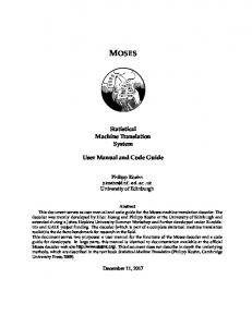
Figure 1: Architecture of the continuous space LM. egy is to divide up the LM training texts into smaller parts, train a LM for each of them and combine these in the SMT system. Two strategies may be employed to combine LMs: One is the use of interpolation. LMs are combined into one by weighting each based on their relevance to the focus domain. The weighting is carried out by optimizing perplexity of a representative tuning set that is taken from the domain. Standard LM toolkits like SRILM (Stolcke, 2002) provide tools to estimate optimal weights using the EM algorithm. The second strategy exploits the log-linear model that is the basis of modern SMT systems. In this framework, a linear combination of feature functions is used, which include the log of the LM probability. It is straight-forward to use multiple LMs in this framework and treat each as a feature function in the log-linear model. Combining several LMs in the log domain corresponds to multiplying the corresponding probabilities. Strictly speaking, this supposes an independence assumption that is rarely satisfied in practice. The combination coefficients are optimized on a criterion directly related to the translation performance, for instance the BLEU score. In summary, these strategies differ in two points: linear versus log-linear combination, and optimizing perplexity versus optimizing BLEU scores.
4 Continuous Space Language Models
sic idea is to convert the word indices to a continuous representation and to use a probability estimator operating in this space. Since the resulting distributions are smooth functions of the word representation, better generalization to unknown n-grams can be expected. This approach was successfully applied to language modeling in small (Schwenk et al., 2006) an medium-sized phrase-based SMT systems (D´echelotte et al., 2007). The architecture of the continuous space language model (CSLM) is shown in Figure 1. A standard fully-connected multi-layer perceptron is used. The inputs to the neural network are the indices of the n−1 previous words in the vocabulary hj =wj−n+1 , . . . , wj−2 , wj−1 and the outputs are the posterior probabilities of all words of the vocabulary: P (wj = i|hj )
662
(1)
where N is the size of the vocabulary. The input uses the so-called 1-of-n coding, i.e., the ith word of the vocabulary is coded by setting the ith element of the vector to 1 and all the other elements to 0. The ith line of the N × P dimensional projection matrix corresponds to the continuous representation of the ith word.1 Let us denote cl these projections, dj the hidden layer activities, oi the outputs, pi their softmax normalization, and mjl , bj , vij and ki the hidden and output layer weights and the corresponding biases. Using these notations, the neural network performs the following operations: dj
= tanh
oi =
X
X
mjl cl + bj
!
(2)
l
vij dj + ki
(3)
j
pi = eoi /
N X
eor
(4)
r=1
The value of the output neuron pi corresponds directly to the probability P (wj = i|hj ). Training is performed with the standard backpropagation algorithm minimizing the following error function: E=
This LM approach is based a continuous representation of the words (Bengio et al., 2003). The ba-
∀i ∈ [1, N ]
N X i=1
1
ti log pi + β
X
m2jl +
jl
Typical values are P = 200 . . . 300
X ij
2 vij
(5)
5 Language Models in Decoding and Re-Ranking LM lookups are one of the most time-consuming steps in the decoding process, which makes timeefficient implementations essential. Consequently,
663
the LMs have to be held in the working memory of the machine, since disk lookups are simply too slow. Filtering LMs to the n-grams which are needed for the decoding a particular sentence may be an option, but is useful only to a degree. Since the order of output words is unknown before decoding, all n-grams that contain any of output words that may be generated during decoding need to be preserved. 0.16 ratio of 5-grams required (bag-of-words)
where ti denotes the desired output. The parameter β has to be determined experimentally. Training is done using a resampling algorithm (Schwenk, 2007). It can be shown that the outputs of a neural network trained in this manner converge to the posterior probabilities. Therefore, the neural network directly minimizes the perplexity on the training data. Note also that the gradient is back-propagated through the projection-layer, which means that the neural network learns the projection of the words that is best for the probability estimation task. In general, the complexity to calculate one probability is dominated by the output layer dimension since the size of the vocabulary (here N =273k) is usually much larger than the dimension of the hidden layer (here H=500). Therefore, the CSLM is only used when the to be predicted word falls into the 8k most frequent ones. While this substantially decreases the dimension of the output layer, it still covers more than 90% of the LM requests. The other requests are obtained from a standard back-off LM. Note that the full vocabulary is still used for the words in the context (input of the neural network). The incorporation of the CSLM into the SMT system is done by using n-best lists. In all our experiments, the LM probabilities provided by the CSLM are added as an additional feature function. It is also possible to use only one feature function for the modeling of the target language (interpolation between the back-off and the CSLM), but this would need more memory since the huge back-off LM must be loaded during n-best list rescoring. We did not try to use the CSLM directly during decoding since this would result in increased decoding times. Calculating a LM probability with a backoff model corresponds basically to a table look-up, while a forward pass through the neural network is necessary for the CSLM. Very efficient optimizations are possible, in particular when n-grams with the same context can be grouped together, but a reorganization of the decoder may be necessary.
0.14 0.12 0.1 0.08 0.06 0.04 0.02 0 0
20
40
60 80 sentence length
100
120
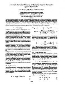
Figure 2: Ratio of 5-grams required to translate one sentence. The graph plots the ratio against sentence length. For a 40-word sentence, typically 5% of the LM is needed (numbers from German–English model trained on Europarl). See Figure 2 for an illustration that highlights what ratio of the LM is needed to translate a single sentence. The ratio increases roughly linear with sentence length. For a typical 30-word sentence, about 4% of the LM 5-grams may be potentially generated during decoding. For large 100word sentences, the ratio is about 15%.2 These numbers suggest that we may be able to use 5–10 times larger LMs, if we filter the LM prior to the decoding of each sentence. SMT decoders such as Moses (Koehn et al., 2007) may store the translation model in an efficient on-disk data structure (Zens and Ney, 2007), leaving almost the entire working memory for LM storage. However, this means for 32-bit machines a limit of 3 GB for the LM. On the other hand, we can limit the use of very large LMs to a re-ranking stage. In two-pass de2
The numbers were obtained using a 5-gram LM trained on the English side of the Europarl corpus (Koehn, 2005), a German–English translation model trained on Europarl, and the WMT 2006 test set (Koehn and Monz, 2006).
English 1.0M 33.8M
300 280
28 Bleu scores
Table 1: Combination of a small in-domain (News Commentary) and large out-of-domain (Europarl) training corpus (number of words). coding, the initial decoder produces an n-best list of translation candidates (say, n=1000), and a second pass exploits additional features, for instance very large LMs. Since the order of English words is fixed, the number of different n-grams that need to be looked up is dramatically reduced. However, since the n-best list is only the tip of the iceberg of possible translations, we may miss the translation that we would have found with a LM integrated into the decoding process.
6 Experiments In our experiments we are looking for answers to the open questions on the use of LMs for SMT: Do perplexity and B LEU score performance correlate when interpolating LMs? Should LMs be combined by interpolation or be used as separate feature functions in the log-linear machine translation model? Is the use of LMs in re-ranking sufficient to increase machine translation performance? 6.1
29
Dev Test
Interpolation
In the WMT 2007 shared task evaluation campaign (Callison-Burch et al., 2007) domain adaptation was a special challenge. Two training corpora were provided: a small in-domain corpus (News Commentary) and the about 30 times bigger out-of-domain Europarl corpus (see Table 1). One method for domain adaptation is to bias the LM towards the indomain data. We train two LMs and interpolate them to optimize performance on in-domain data. In our experiments, the translation model is first trained on the combined corpus without weighting. We use the Moses decoder (Koehn et al., 2007) with default settings. The 5-gram LM was trained using the SRILM toolkit. We only run minimum error rate training once, using the in-domain LM. Using different LMs for tuning may change our findings reported here. When interpolating the LMs, different weights
664
260
27
240
26
220
25 Dev perplexity
200
BLEU score
French 1.2M 37.5M
Perplexity
News Commentary Europarl
24
180 0
0.2
0.4 0.6 0.8 Interpolation coefficient
1
Figure 3: Different weight given to the out-ofdomain data and effect on perplexity of a development set (nc-dev2007) and on the B LEU score of the test set (nc-devtest2007). TM combined combined 2 features 2 features
LM 2 features interpolated 0.42 2 features interpolated 0.42
BLEU (test) 27.30 27.23 27.64 27.63
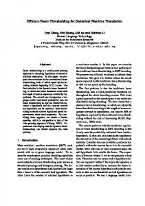
Table 2: Combination of the translation models (TM) by simple concatenation of the training data vs. use of two feature functions, and combination of the LM (LM) by interpolation or the use of two feature functions. may be given to the out-of-domain versus the indomain LM. One way to tune the weight is to optimize perplexity on a development set (nc-dev2007). We examine values between 0 and 1, the EM procedure gives the lowest perplexity of 193.9 at a value of 0.42. Does this setting correspond with good B LEU scores on the development and test set (ncdevtest2007) ? See Figure 3 for a comparison. The B LEU score on the development data is 28.55 when the interpolation coefficient is used that was obtained by optimizing the perplexity. A slightly better value of 28.78 good be obtained when using an interpolation coefficient of 0.15. The test data seems to be closer to the out-of-domain Europarl corpus since the best BLEU scores would be obtained for smaller values of the interpolation coefficient. The second question we raised was: Is interpolation of LMs preferable to the use of multiple LMs
as separate feature functions. See Table 2 for numbers in the same experimental setting for two different comparisons. First, we compare the performance of the interpolated LM with the use of two feature functions. The resulting B LEU scores are very similar (27.23 vs. 27.30). In a second experiment, we build two translation models, one for each corpus, and use separate feature functions for them. This gives a slightly better performance, but again it gives almost identical results for the use of interpolated LMs vs. two LMs as separate feature functions (27.63 vs. 27.64). These experiments suggest that interpolated LMs give similar performance to the use of multiple LMs. In terms of memory efficiency, this is good news, since an interpolated LM uses less memory. 6.2
Re-Ranking
Let us now turn our attention to the use of very large LMs in decoding and re-ranking. The largest freely available training sets for MT are the corpora provided by the LDC for the NIST and G ALE evaluation campaigns for Arabic–English and Chinese– English. In this paper, we concentrate on the first language pair. Our starting point is a system using Moses trained on a training corpus of about 200 million words that was made available through the G ALE program. Training such a large system pushes the limits of the freely available standard tools. For instance, GIZA++, the standard tool for word alignment keeps a word translation table in memory. The only way to get it to process the 200 million word parallel corpus is to stem all words to their first five letters (hence reducing vocabulary size). Still, GIZA++ training takes more than a week of compute time on our 3 GHz machines. Training uses default settings of Moses. Tuning is carried out using the 2004 NIST evaluation set. The resulting system is competitive with the state of the art. The best Corpus Parallel training data (train) AFP part of Gigaword (afp) Xinhua part of Gigaword (xin) Full Gigaword (giga)
Words 216M 390M 228M 2,894M
Table 3: Size of the training corpora for LMs in number of words (including punctuation)
665
Px Bleu score Decode LM eval04 eval04 eval06 3-gram train+xin+afp 86.9 50.57 43.69 3-gram train+giga 85.9 50.53 43.99 4-gram train+xin+afp 74.9 50.99 43.90 Reranking with continuous space LM: 5-gram train+xin+afp 62.5 52.88 46.02 6-gram train+xin+afp 60.9 53.25 45.96 7-gram train+xin+afp 60.5 52.95 45.96 Table 4: Improving MT performance with larger LMs trained on more training data and using higher order of n-grams (Px denotes perplexity). performance we obtained is a B LEU score of 46.02 (case insensitive) on the most recent eval06 test set. This compares favorably to the best score of 42.81 (case sensitive), obtained in 2006 by Google. Casesensitive scoring would drop our score by about 2-3 B LEU points. To assess the utility of re-ranking with large LMs, we carried out a number of experiments, summarized in Table 4. We used the English side of the parallel training corpus and the Gigaword corpus distributed by the LDC for language modeling. See Table 3 for the size of these corpora. While this puts us into the moderate billion word range of large LMs, it nevertheless stresses our resources to the limit. The largest LMs that we are able to support within 3 GB of memory are a 3-gram model trained on all the data, or a 4-gram model trained only on train+afp+xin. On disk, these models take up 1.7 GB compressed (gzip) in the standard ARPA format. All these LMs are interpolated by optimizing perplexity on the tuning set (eval04). The baseline result is a B LEU score of 43.69 using a 3-gram trained on train+afp+xin. This can be slightly improved by using either a 3-gram trained on all data (B LEU score of 43.99) or by using a 4-gram trained on train+afp+xin (B LEU score of 43.90). We were not able to use a 4-gram trained on all data during the search. Such a model would take more than 6GB on disk. An option would be to train the model on all the data and to prune or quantize it in order to fit in the available memory. This may give better results than limiting the training data. Next, we examine if we can get significantly better performance using different LMs in re-ranking.
To this end, we train continuous space 5-gram to 7gram LMs and re-rank a 1000-best list (without duplicate translations) provided by the decoder using the 4-gram LM. The CSLM was trained on the same data as the back-off LMs. It yields an improvement in perplexity of about 17% relative. With various higher order n-grams models, we obtain significant gains, up to just over 46 B LEU on the 2006 NIST evaluation set. A gain of over 2 B LEU points underscores the potential for reranking with large LM, even when the baseline LM was already trained on a large corpus. Note also the good generalization behavior of this approach : the gain obtained on the test data matches or exceeds in most cases the improvements obtained on the development data. The CSLM is also very memory efficient since it uses a distributed representation that does not increase with the size of training material used. Overall, about 1GB of main memory is used.
7 Discussion In this paper we examined a number of issues regarding the role of LMs in large-scale SMT systems. We compared methods to combine training data from diverse corpora and showed that interpolation of LMs by optimizing perplexity yields similar results to combining them as feature functions in the log-linear model. We applied for the first time continuous space LMs to the large-scale Arabic–English NIST evaluation task. We obtained large improvements (over 2 B LEU points) over a strong baseline, thus validating both continuous space LMs and re-ranking as a method to exploit large LMs. Acknowledgments This work has been partially funded by the French Government under the project I NSTAR (ANR JCJC06 143038) and the DARPA Gale program, Contrat No. HR0011-06-C-0022 and the EuroMatrix funded by the European Commission (6th Framework Programme).
References Yoshua Bengio, Rejean Ducharme, Pascal Vincent, and Christian Jauvin. 2003. A neural probabilistic language model. JMLR, 3(2):1137–1155.
666
Thorsten Brants, Ashok C. Popat, Peng Xu, Franz J. Och, and Jeffrey Dean. 2007. Large language models in machine translation. In EMNLP, pages 858–867. Chris Callison-Burch, Cameron Fordyce, Philipp Koehn, Christof Monz, and Josh Schroeder. 2007. (Meta-) evaluation of machine translation. In Second Workshop on SMT, pages 136–158. Daniel D´echelotte, Holger Schwenk, Hlne BonneauMaynard, Alexandre Allauzen, and Gilles Adda. 2007. A state-of-the-art statistical machine translation system based on Moses. In MT Summit. Ahmad Emami, Kishore Papineni, and Jeffrey Sorensen. 2007. Large-scale distributed language modeling. In ICASSP. Marcello Federico and Nicola Bertoldi. 2006. How many bits are needed to store probabilities for phrasebased translation? In First Workshop on SMT, pages 94–101. Philipp Koehn and Christof Monz. 2006. Manual and automatic evaluation of machine translation between European languages. In First Workshop on SMT, pages 102–121. Philipp Koehn et al. 2007. Moses: Open source toolkit for statistical machine translation. In ACL Demo and Poster Sessions, pages 177–180, June. Philipp Koehn. 2005. Europarl: A parallel corpus for statistical machine translation. In MT Summit. Holger Schwenk, Marta R. Costa-juss`a, and Jos´e A. R. Fonollosa. 2006. Continuous space language models for the IWSLT 2006 task. In IWSLT, pages 166–173. Holger Schwenk. 2007. Continuous space language models. Computer Speech and Language, 21:492– 518. Andreas Stolcke. 2002. SRILM - an extensible language modeling toolkit. In ICSLP, pages II: 901–904. David Talbot and Miles Osborne. 2007a. Randomised language modelling for statistical machine translation. In ACL, pages 512–519. David Talbot and Miles Osborne. 2007b. Smoothed Bloom filter language models: Tera-scale LMs on the cheap. In EMNLP, pages 468–476. Richard Zens and Hermann Ney. 2007. Efficient phrasetable representation for machine translation with applications to online MT and speech translation. In NACL, pages 492–499. Ying Zhang, Almut Silja Hildebrand, and Stephan Vogel. 2006. Distributed language modeling for n-best list re-ranking. In EMNLP, pages 216–223.