TELKOMNIKA Indonesian Journal of Electrical Engineering Vol.12, No.1, January 2014, pp. 10 ~ 19 DOI: http://dx.doi.org/10.11591/telkomnika.v12i1.2729
10
Latin Hypercube Sampling with Evolutionary Algorithm for Static Security Risk Assessment Junfang Li The Research Centre of Power Grid Plan/Guangdong Power Grid Co., Ltd. Dongfengdong Road, No. 757, Guangzhou, 510080, China e-mail:
[email protected]
Abstract Due to correlation coefficient matrix of initialized samples are not always positive definite, this paper presents the improved Latin Hypercube Sampling (LHS) methods with Evolutionary Algorithm (EA) to control correlation and handle power system probability analysis problem. To deal with the non-positive definite correlation matrix, an improved median Latin hypercube sampling with evolutionary algorithm (EA) called MLHS-EA into Monte Carlo simulationis proposed and investigatedusing IEEE 118-bus system with wind farms. This paper also discusses the misunderstandings about the non-positive definite correlation matrix and application of LHS in power system probabilistic analysis. With the proposed method in this paper, the correlation can be controlledmore effectively than previous LHS methods. The accuracy of LHSfor the static security assessment can also be improved further for solving the probabilistic analysis problem in power system. The effectiveness of the method is validated with the Matlabsimulation results. Keywords: Latin hypercube sampling, risk assessment, evolutionary algorithm, power system Copyright © 2014 Institute of Advanced Engineering and Science. All rights reserved.
1. Introduction To evaluate theimpact of the load forecasting uncertainty on power systems’ security, probabilistic analysis of the static security risk has attracted a large amount of interest from 1990s to recent years [1]-[3]. The probabilistic load flow (PLF) proposed by Borkowska in 1974 in[4] can be adopted to calculate the risk indices of line overload and bus over-voltage to evaluate the potential static security risk and weak points in power system.Monte Carlo simulation (MCS) [1]-[3], [5] is the most accurate, flexible and robust method when samples are enough. The theory of MCSwith variance reduction technique is introduced in [3], [6],[7], better than MCS with simple random sampling (SRS). For a deterministic function Yf(X), where YR and XRK and f(·) is expensive to compute which may use a more complicated sampling scheme, McKay et al. described Latin hypercube sampling (LHS) first in 1979 [8]. LHS is a stratified sampling with a great merit in solving this problem with high efficiency. LHS has two steps: sampling and correlation control. The Median LHS (MLHS)to select the midpoint of each interval is the dominant approach. Correlation controlto reduce undesired random correlation and to introduce prescribed correlation is important [9], because the correlation between the input variables has a profound impact on the uncertainty of the outputs. Combined with correlation control methods, the LHS methodshave many variants:LHS with Rank Gram-Schmidt(RGS) [9], LHS with random permutation (LHSRP) [10], LHS withCholesky decomposition [11], [12], optimal LHS [13], LHS with Genetic Algorithm (GA) or columnwise-pairwise (CP) [14], LHS with simulated annealing [15] and single-switch-optimized sample ordering scheme (SSO) [16]. The performance in [14] indicates that CP methods are most efficient for small and medium size Latin hypercube, while an adopted GA performs better for large Latin hypercube. Crossover operator is important in GA. However, to a specified problem like PLF, it’s difficult to use crossover operator. Based on the research on the quasiMonte Carlosimulation, Latin hypercube Hammersley sequence sampling (LHHS)was developed [17]. LHHS generates the sample values with LHS and pairs these values with Hammersley sequence sampling (HSS) [17], [18]. LHHS needs enough prime numbers for different random variables. This fact limits its application when a problem has the high-
Received March 21, 2013; Revised July 6, 2013; Accepted September 8, 2013
11
ISSN: 2302-4046
TELKOMNIKA
dimensional random variables. Theoretically, the consistency and unbiasedness about LHS with dependence are proved in [19]. The input distribution type for LHS methods is summarized [20]. The Cholesky decomposition needs that the correlation coefficient matrix is a positive definite matrix. However, in real applications, of input random variables can be non-positive definitewhen obtained by the samples in the first step. In this paper, to improve the correlation control of LHS effectively when the correlation matrix is a non-positive definite matrix, correlation controlled bythe Evolutionary Algorithm (EA) is presented. Many previous literatures in [21] rarely take into account the generator’s reactive output constraint when calculating PLF. This paper considers the reactive power limit of the generators and the independence in different nodes when evaluating the steady-state security risk. The remainder of the paper is organized as follows. Section II introduces the related background of LHS, presents the improved methods and analyzes the correlation matrix aftersampling in the first step. Section III describes the simulation in the static risk assessment. Section IV appliesthe methods inIEEE30- and 118-bus system. Section V concludes the paper.
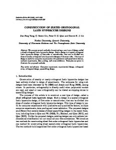
2. The Proposed Method 2.1. Related Background of Latin Hypercube Sampling The main idea of MLHS is described as follows. Let Yk is the cumulative distribution function of Xk, namely YkFk(Xk), Xk{X1,…,XK}. Then the domain of each variable is divided into equal probable separated intervals, and one sample value of Xk is selected from each interval directly from Yk, namelyXk=Fk1(Yk).In MLHS method, due to adopting the midpoint value from each interval, the nth sample of Xk is chosen according to xk,n=Fk1((n-0.5)/N).Assume that the cumulative distribution curves of two random variables following normal distribution N(10MW,(4MW)2) are divided into N equal sections, respectively, and N=6. The cumulative distribution function (CDF) and probabilistic distribution function (PDF)of the random variable are shown in Figure1(a)-(b), respectively.
(a) CDF (b) PDF
Figure 1. Sampling of MLHS, LHSRP method In Figure 1(a), x1,kn and x2,kn represent the random pointusing MLHSand LHSRP, respectively. Forthree LHS methods, the random point in each interval is determined as follows. 1
MLHS [12]: x1,kn Fk
n 0.5 N 1
LHSRP [22]: x2,kn Fk 1
rk ,n
(1)
N ( n 1) N
(2)
(3) LHHS [18]: xH,kn Fk hk ,n N ( n 1) N The roles of parameter rk,n and hk,n are the random number generators in [0, 1]. The value of rk,n is a pseudo-random number. The value of parameter hk,n is from the Hammersley points. The details on the process to generate the Hammersley points can be found in [18]. For all LHS methods, the CDF of the input variable must be strictly increasing continuous function to ensure that the inverse function exists. TELKOMNIKA Vol. 12, No. 1, January 2014: 10 – 19
ISSN: 2302-4046
12
2.2. Description of EA for Correlation Control The correlation control can be achieved by the permutation method. The main process of the EA is that random permutation for enough times and taking the best one when theobjective correlation reaches an acceptable value. Inspired by the asexual propagation, the optimization permutation is called as “EA”. The size of chromosomes represents the number of random variables. Each chromosome has the same size of genes, namely the sample size N. The fitness function evaluation is a minimization optimization problem of objective correlation function.The gene has a mutation behavior. In the context of the EA paradigm, mutation is seen as a change with a random element [23]. Thus, the update or change of the arrangement by a random permutation of N sampled values of Xkis called as “mutation”.“Selection” means that the specific generation with a smaller objective value than all previous generations is selected as the best generation to survive, andthe previous generations are eliminated. Let X1,…,XKbe a group of random variables and construct a K-dimensional random vector X=[X1,…,XK]T. Each random variable has Nsampling values, and constructs a K×N sampling matrixM.The covariance of random variables Xi and Xjis defined as:
cij E ([ X i E ( X i )][ X j E ( X j )])
(4)
The correlation coefficient ij between Xi and Xj are defined by Pearson product-moment correlation coefficient:
ij
cij
(5)
cii c jj
The correlation matrix with elements ijis symmetric. Before correlation control, two situations need to be distinguished. Situation 1: of the independent variables can be denoted by an identity matrix. Situation 2: an objective correlation matrix *has most of elementsij(i≠j) in the interval (0, 1) or (-1, 0). Situation 1 is possible to happen in power system. The predetermined objective correlation matrix * in Situation 2 in a bulk system is unrealistic. The reason for this is that it’s very difficult to accurately give all realistic or approximately realistic non-diagonal elements in advance for a K×Kmatrix * and ensure * a positive definite matrix when K value is high. For example, in the IEEE 118-bus system, there are 99 active loads. If Situation 2 is considered, the matrix * has 99×99 elements. To accurately give more than 9000 non-diagonal elements in the interval (0, 1) and ensure the positive definite matrix is unrealistic. Thus, the Situation 2 is unrealistic. In a bulk system, the forecasting uncertainties of some load nodes are considered as approximate independent. The loads with a correlation coefficientequaling one can be denoted by linear correlation. The correlation matrix is an identity matrix. The optimization problem in the correlation control has afitness function. To solve the situation 1, because completely independent variables strictly satisfying the correlation coefficient element ij=0(i≠j) are not easy to achieve, but approximate to zero. updating the sample permutation to get a minimum value of correlation objective function, Thus, the root mean square correlation among X1,…,XKis adopted as the objective function, that is, K
j 1
min s 2 ij2 / [( K 1) K ]
(6)
j 2 i 1
The objective function s represents the root mean square value of off-diagonal lower triangular or upper triangular elements of . If s is close to zero, the correlation between variables is small. The direction of mutation is to get a new arrangement with a minimum objective value s. The objective function s is calculated using the updated sampling matrix M.
Latin Hypercube Sampling with Evolutionary Algorithm for Static Security Risk ... (Junfang Li)
13
ISSN: 2302-4046
TELKOMNIKA
2.3. Steps of LHS Method with EA The above three LHS methods with EA can be denoted by MLHS-EA, LHSRP-EA and LHHS-EA. Assume there are K random variables. For the above-mentioned Situation 1, the steps of LHS with EA are as follows. Step 1: Generate an initialized K×N sampling matrix M0 for one of three LHS methods according to the Eq. (1)-(3). It can be deduced that the elements of M0 are sorted in an ascending order from the Eq. (1). Take MLHS-EA for example:
x1,11 x 1,21 M0 = x1, K 1
x1,12 x1,22 x1, K 2
x1,1N x1,2 N x1, KN K N
(7)
Step 2: Calculate the initialized correlation matrix of the matrix M0. For example, using MLHS-EA, IEEE 14-, 30-, 57- and 118-bus systems are tested after the first step. Thematrix is found to be a non-positive definite matrix with all elements equalling one, namely:
1 1 1
1 1 1 1 1 1 K K
(8)
If using LHSRP-EA, IEEE 14-, 30-, 57- and 118-bus systems are found that the offdiagonal elements of are all in the interval (0.9, 1.0), and very close to one. Step 3: Control correlation using EA. Set the maximum generation is G, and initialize the objective function value smin=1. The matrix Mg in the gth generation (1≤g≤G) can be seen as a cell. Each row of the cell is a chromosome with N genes. Thus, the cell Mg has K chromosomes and total K×Ngenes. After each evolution, the sequence of genes in each chromosome will be sorted randomly again. For example, the Mg evolves to be the following form after gth iterations.
x1,1N x 1,22 Mg = x1, KN
x1,11
x1,13
x1,21
x1,2 N
x1, K 2
x1, K 3
x1,12 x1,23 x1, K 1 K N
(9)
Then calculate the s in the gth generation. If s≤smin, set smin=s. Step 4: Continue iterations when g1, positive integer), are yN-1 and yN, respectively, the percentage changing rate r is calculated as Eq. (17). Criterion B: Each output random variable’ sample variance is within 0.01% of the expected value in above 90% probability.
r y N y N 1 100% y N 1
(17)
Referring to the previous articles [12], [16], for IEEE 118-bus system, 30000 times of MCS with SRS for the PLF is enough.
4. Results and Discussion The validity of the proposed method in the static risk assessment is demonstrated on IEEE 118-bus system. The program is developed with MATPOWER 4.0 on Dual Core 2.71GHz PC with 1.75G of RAM. The wind power and the load are seen as independentrandom variables. The forecasted wind power values from different wind farms are independent.The wind power uncertainty is modelled as Beta distribution [24], the mean value of which equals the average forecasted power and the standard deviation is estimated as 30% of the mean value. The nodal active and reactive power distributions of loads follow normal distribution.The mean value is the same as the original data provided byMATPOWER 4.0. And the standard deviation of loadis equal to10% ofthe mean value, namely =10%. 4.1. IEEE 30-bus System For testing the efficiency of controlling correlation, take IEEE 30-bus system for example. The numerical data are from MATPOWER 4.0.The curves of s and η of the four methods are shown in Figure 2 (a)-(b).When N=50, the results are acceptable. The computation time for LHSRP, LHHS, MLHS-EA and LHIS-EA when N=50 is 2.37s, 2.31s, 1.94s, 1.97s, respectively.From Figure 2, the correlation can be controlled with EA better than without EA.
(a)s obtained by four methods with and without EA
(b) Comparison of ofs by four methods with and without EA
Figure 2. Comparison of effectiveness of correlation control by EA TELKOMNIKA Vol. 12, No. 1, January 2014: 10 – 19
ISSN: 2302-4046
16
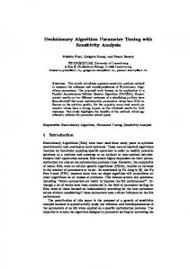
4.2. Modified IEEE 118-bus System with Wind Farms IEEE 118-bus system has 186 lines, shown in Figure 3. There are 189 independent input random variables including 99 active loads and 90 reactive loads. The test system has been modified to include three wind farms having all Doubly Fed Induction Generators in nodes 10, 65 and 89, respectively. Wind power replaces part of the conventional generation in the three nodes, e.g., 120 MW wind power in node 10, 180 MW wind power in node 65, and 162 MW wind power in node 89. After wind power integrated into 118-bus system, the capacities of the thermal units in the nodes 10, 65 and 89 are 330MW, 211MW and 445MW, respectively. [Umin, Umax]=[0.95pu, 1.05pu], and [Pfmin,Pfmax]=[-500MW, 500MW]. We assume that the total rated power of each wind farm is 300MW. The parameters of Beta distribution for each wind farm calculated according to [24] are given in Table 1. The Beta distributions are shown in Figure4. In EA, G=1000. In MLHS, the sample size N is 300. The error of the expected value of voltage magnitude in each node is shown in Figure 5. The indices RiskU and SevU of the first three nodes in a descending order are given in Table 2.The indices RiskLF and SevLF of the first three lines in a descending order are given in Table 3. To analyze the influence of load and wind power uncertainties on the load flow, the situation of =10% is compared with =1%. The indices RiskU and SevU of the first three nodes in a descending order are given in Table 4. The CDF curves of voltage magnitude in node 53 and node 118 are shown in Figure 6. Table 1. The Statistical Parameters for Wind Farms in the Node 10, 65 and 89 Mean (p.u.) Std. (p.u.) Beta distribution Rated power (MW)
Node 10 0.4 0.12 β(6.27, 9.40) 300
Node 65 0.6 0.18 β(3.84, 2.56) 300
Node 89 0.54 0.162 β(4.57, 3.89) 300
Table 2. Sorting table of RiskUand SevU when loads satisfy =10% No. 1 2 3
Node 53 118 2
RiskU 0.9933 0.7100 0
No. 1 2 3
Node 53 118 21
SevU 1.1848 1.0716 0.9660
Table 3. Sorting table of RiskLFand SevLF when loads satisfy =10% No. 1 2 3
Line 9-10 8-9 1-2
RiskLF 0.0667 0.0500 0
No. 1 2 3
Line 9-10 8-9 8-5
SevLF 1.0966 1.0827 0.7516
Table 4. Sorting table of RiskUand SevU when loads satisfy =1% No. 1 2 3
Node 53 118 2
RiskU 1 1 0
No. 1 2 3
Node 53 118 9
SevU 1.0907 1.0193 0.9215
Latin Hypercube Sampling with Evolutionary Algorithm for Static Security Risk ... (Junfang Li)
17
ISSN: 2302-4046
TELKOMNIKA
Figure 3. Wind farms in node 89, 65 and 10 in IEEE 118-bus system
Figure 4. Beta distribution
Figure 5. Error of μof voltage magnitudein 118 nodes
Figure 6. CDF of voltage magnitudes of node 53 and 118 in wind integrated power system
TELKOMNIKA Vol. 12, No. 1, January 2014: 10 – 19
ISSN: 2302-4046
18
4.3. Results Analysis The computation time using MLHS-EA is 8.4 seconds. The expected values of voltage magnitude and active power flow obtained by MLHS-EA for the PLF have error about 0.067% and 2.027%, respectively. The reason for only giving the indices of the first three nodes in Table 2 and Table 3 is that the RiskU of other nodes after the first three nodes are all zero. From Table 2 and Table 3, the nodes 53 and 118 have very high possibilities of over-voltage and severity degree. The lines 9-10 and 8-9 have small possibilities of overload but high severity degree. In Figure 5, the maximum error of the expected values of voltage magnitudes in all 118 nodes is less than 1%. As shown in Figure 6, Table 2 and Table4, the nodes 53 and 118 have high crisis. If the fault events are considered, the system has great crisis. Thus, a prevention control to keep voltage security is necessary. The results show that LHS with EA is effective to solve the PLF problem when the correlation matrix obtained after the sampling initialization is non-positive definite. For a large-scale power system with most independent random variables, the improved methods are effective. 4.4. Discussion This section aims at discussing the misunderstandings about the application of LHS in power system probabilistic analysis. These misunderstandings and questions are as follows: (1) Why the correlation matrix is non-positive definite? Why not generate a positive definite matrix that could be done by the Cholesky decomposition? The answer is that the matrix is the correlation matrix of the matrix M0 formed by the sampling rule (i.e. Eq. (1), (2) and (3)) in the first step of LHS. The sample points are all naturally sorted in an increasing form. The correlation matrix is obtained by calculation, not given in advance. The calculated matrix after the first step using MLHS is a non-positive matrix that can’t be done by Cholesky decomposition. The random variables are completely correlated in the first step. Because the precondition of the PLF problem is that the random variables are independent, it needs to control correlation to make the sample matrix M satisfy the precondition. That is the reason why use EA, not Cholesky decomposition to control correlation in the second step. (2) There exist rare nodes with high errors of expected values of voltage magnitudes, or rare lines with high errors of expected values of active power flow when other nodes or lines have all statistical results with very small errors. Does this show no benefit of using LHS-EA? The answer is that rare nodes or lines with high errors are realistic, especially for a random variable with a very low actual value. For example, if the actual statistical result ±of the voltage magnitude in a node is 0.9871±0.0005pu, and the result obtained using LHS is 0.9881±0.0004pu, it can be found thatusing Eq. (15), the relative error of is 0.1%, and the relative error of is 20% (i.e. |0.0004-0.0005|/0.0005). Because the relative error rate (i.e. /)is quite small, i.e. /=5×10-4, the relative error of has no influence on judging the performance of LHS-EA. IEEE 30-, 57-bus system are also tested and found that the phenomena is very common. Thus, it should pay great attention to the authenticity of the results. The phenomena with high error for rare nodes or lines can’t deny the validity of LHS with EA.
5. Conclusion This paper presents the improved LHS methods with Evolutionary Algorithm to control correlation and handle power system static security risk assessment problem. To deal with the non-positive definite correlation matrix, an improved median Latin hypercube sampling with EA called MLHS-EA into Monte Carlo simulation is proposed and investigatedusing modified IEEE 118-bus systemwith wind farms in this paper. With the method proposed in this paper, the correlation is effectively controlled and the accuracy of the LHSfor the static security assessment can be improved further than previous LHS methods. The methods can be usedfor solving the probabilistic analysis problem in power system.
Latin Hypercube Sampling with Evolutionary Algorithm for Static Security Risk ... (Junfang Li)
19
ISSN: 2302-4046
TELKOMNIKA
References [1] JD McCalley, V Vittal and N Abi-Samra. An overview of risk based security assessment. IEEE Power Engineering Society Summer Meeting. July 18-22, Edmonton, Canada. 1999; 1: 173-178. [2] F Xiao and JD McCalley. Power system risk assessment and control in a multiobjective framework. IEEE Trans. on Power Syst. 2009; 24(1): 78–85. [3] DS Kirschen, D Jayaweera, DP Nedic, et al. A probabilistic indicator of system stress. IEEE Trans. on Power Syst., 2004; 19(3): 1650–1657. [4] B Borkowska. Probabilistic load flow.IEEE Trans. Power App. Syst. 1974; PAS-93(3): 752–759. [5] W Li. Risk Assessment of Power Systems: Models, Methods, and Applications. New York: IEEE Press/Wiley. 2004: 79–86. [6] A Breipohl, FN Lee, J Huang et al. Sample size reduction in stochastic production simulation. IEEE Trans. Power Syst. 1990; 5(3): 984–992. [7] Z Bie and X Wang. Studies on variance reduction technique of Monte Carlo simulation in composite system reliability evaluation. Electric Power Systems Research. 2002; 63(1): 59–64. [8] MD Mckay, RJ Beckman, and WJ Conover. A comparison of three methods for selecting values of input variables in the analysis of output from a computer code.Technometrics. 1979; 21(2): 239–245. [9] AB Owen. Controlling correlations in Latin hypercube samples. Journal of the American Statistical Association. 1994; 89(428): 1517–1522. [10] P Jirutitijaroen and C Singh. Comparison of simulation methods for power system reliability indexes and their distributions. IEEE Trans. Power Syst. 2008; 23(2): 486–493. [11] RL Iman and WJ Conover. A distribution-free approach to inducing rank correlation among input variables.Commun. Statist. –Sim. Comput. 1982; 11(3): 311–334. [12] H Yu, CY Chung, KP Wong et al. Probabilistic load flow evaluation with hybrid Latin hypercube sampling and Cholesky decomposition. IEEE Trans. Power Syst. 2009; 24(2): 661–667. [13] Jeong-Soo Park. Optimal latin-hypercube designs for computer experiments. Journal of Statistical Planning and Inference. 1994; 39(1): 95–111. [14] M Liefvendahl and R Stocki. A study on algorithms for optimization of Latin hypercubes. Journal of Statistical Planning and Inference. 2006; 136(9): 3231–3247. [15] M Vořechovský and D Novák. Correlation control in small-sample Monte Carlo type simulations I: A simulated annealing approach. Probabilistic Engineering Mechanics. 2009; 24(3): 452–462. [16] DE Huntington and CS Lyrintzis. Improvements to and limitations of Latin hypercube sampling. Probabilistic Engineering Mechanics. 1998; 13(4): 245–253. [17] JR Kalgnanam and UM Diwekar. An efficient sampling technique for off-line quality control. Technometrics. 1997; 39(3): 308–319. [18] Urmila M Diwekar. A novel sampling approach to combinatorial optimization under uncertainty. Computational Optimization and Applications. 2003; 24(2-3): 335–371. [19] Packham, Natalie and Schmidt, Wolfgang M. Latin Hypercube Sampling with Dependence and Applications in Finance.Germany: Frankfurt School of Finance & Management, 2008: 1-23. [20] LP Swiler and GD Wyss. A user’s guide to Sandia’s Latin hypercube sampling software: LHS Unix Library/standalone version. Sandia National Laboratories, Albuquerque, NM. Technical Report SAND 2004–2439. [21] P Chen, Z Chen, and B Bak-Jensen.Probabilistic load flow: a review. The 3rd International Conference on Electric Utility Deregulation and Restructuring and Power Technologies. Nanjing, China. 2008; 1: 1586-1591. [22] R Wang, Urmila Diwekar, Catherine E Grégoire Padró. Efficient sampling techniques for uncertainties in risk analysis. Environmental Progress. 2004; 23(2): 141–157. [23] S Das and PN Suganthan. Differential evolution: A survey of the state-of-the-art. IEEE Trans. on Evolutionary Computation. 2011; 15(1): 4–30. [24] Usaola J. Probabilistic load flow in systems with wind generation.Generation, Transmission & Distribution, IET. 2009; 3(12): 1031–1041.
TELKOMNIKA Vol. 12, No. 1, January 2014: 10 – 19