Laughter Classification Using Deep Rectifier Neural

c 2016 by PAN – IPPT Copyright

ARCHIVES OF ACOUSTICS

DOI: 10.1515/aoa-2016-0064

Vol. 41, No. 4, pp. 669–682 (2016)

Laughter Classification Using Deep Rectifier Neural Networks with a Minimal Feature Subset Gábor GOSZTOLYA(1) , András BEKE(2) , Tilda NEUBERGER(2) , László TÓTH(1) (1)

MTA-SZTE Research Group on Artificial Intelligence of the Hungarian Academy of Sciences and University of Szeged Szeged, Hungary; e-mail: {ggabor, tothl}@inf.u-szeged.hu (2)

Research Institute for Linguistics of the Hungarian Academy of Sciences Budapest, Hungary; e-mail: {beke.andras, neuberger.tilda}@nytud.mta.hu (received January 27, 2016; accepted June 23, 2016 )

Laughter is one of the most important paralinguistic events, and it has specific roles in human conversation. The automatic detection of laughter occurrences in human speech can aid automatic speech recognition systems as well as some paralinguistic tasks such as emotion detection. In this study we apply Deep Neural Networks (DNN) for laughter detection, as this technology is nowadays considered state-of-the-art in similar tasks like phoneme identification. We carry out our experiments using two corpora containing spontaneous speech in two languages (Hungarian and English). Also, as we find it reasonable that not all frequency regions are required for efficient laughter detection, we will perform feature selection to find the sufficient feature subset. Keywords: speech recognition; speech technology; computational paralinguistics; laughter detection; deep neural networks.

1. Introduction Non-verbal communication plays an important role in human speech comprehension. Speakers detect information in different sensory modalities (auditory and visual channels) simultaneously during everyday interactions. Besides the visual cues (gestures, facial expressions, eye contact, etc.), some types of messages can be transferred by non-verbal vocalizations (laughter, throat clearing, breathing) as well. The interpretation of speakers’ intentions can be assisted by using paralinguistic information; for instance, to acquire information about the speakers’ emotional state and attitudes, or to recognize equivocation and irony. The automatic detection of laughter could be utilized in a number of ways. For example, laughter detection could assist the determination of speaker emotion (Suarez et al., 2012), or it could be used to search for videos with a humorous content. Incorporating laughter detection in automatic speech recognition (ASR) systems could also help reduce the word error rate by identifying non-speech sounds.

Since their invention a decade ago, Deep Neural Networks (DNN) have gradually replaced traditional Gaussian Mixture Models (GMMs) as the state-of-theart method in the phoneme classification (or phoneme likelihood estimation) subtask of ASR. The main reason for this was because they performed more accurately. Of course, the fact that they are able to handle the large number of examples appearing in this task, and that they can provide high-quality phoneme likelihood estimates (unlike some other state-of-the-art machine learning methods like AdaBoost.MH (Schapire, Singer, 1999) and Support-Vector Machines (SVM ¨ lkopf et al., 2001))) have also played a role in (Scho their success. As the frame-level laughter detection task is quite similar to the phoneme classification one, in this study we shall apply DNNs to laughter classification. We will utilize three popular feature sets, namely MelFrequency Cepstral Coefficients (MFCCs), Perceptual Linear Predictions (PLP) and raw Mel-scale filter bank energies (FBANK). We will perform our experiments on two databases containing laughter segments.

Unauthenticated Download Date | 12/28/16 2:12 PM

670

Archives of Acoustics – Volume 41, Number 4, 2016

The first contains Hungarian speech recorded in a clean environment, while the second consists of English telephone conversations. Phoneme classification appears to be a more complicated task than laughter classification. Therefore, it is quite likely that a feature set developed for the former task is overcomplete for the latter one. With this in mind, we will also perform feature selection to find out which frame-level attributes are actually useful for laughter detection. We will also test the robustness of the selected feature subsets by performing cross-corpus evaluations.

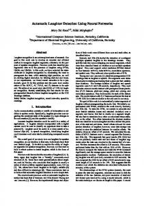
is usually like those of breathy CV syllables (e.g., /hV/ syllable). See Fig. 1 for an oscillogram and spectrogram of a spontaneous laughter.

2. Automatic laughter detection Spontaneous conversations frequently contain various non-verbal vocalizations (hesitation, breathing, throat clearing); laughter is one of the most frequent non-verbal vocalizations. Studies showed that laughter occurs 1–3 times per minute in conversational speech (Holmes, Marra, 2002). However, it is important to note that many factors influence the occurrences of laughter, such as context, speech topic, level of acquaintanceship, hierarchy, culture and personality of the speakers. Laughter is an inborn, species-specific indicator of affection, which is socially constituted and easily decodable. Laughter has been investigated by researchers coming from various fields including psychology, sociology, ethology and linguistics. Across species, laughlike vocalizations appear to signal positive affect and affiliation; and might also be a reliable signal that the producer of the vocalization is unlikely to attack. In humans, spontaneous laughter has important functions in signaling positive affect and cooperative intent (Bryant, Aktipis, 2014). Laughter has also various functions in everyday conversations. It can be a part of social interaction in early infancy (Nwokah et al., 1993), a part of appeasement in situations of dominance/subordination, ¨nger et al., or a part of aggressive behavior (Rothga 1998). It can serve to regulate the flow of the interaction, to mitigate the semantic context of the preceding utterance, or it can function as a stress-reducing strategy. It can also provide cues to the semantic content of utterances in conversations, such as jokes or topic changes and can indicate the boundary of the turns; hence, laughter and other non-verbal sounds are of increasing interest in discourse analysis, e.g. (Glenn, 2003; Gunther, 2002). Laughter has been analyzed on the one hand in relation to the psychology of humor, e.g. (Goldstein, McGhee, 1972; Martin, 2007), and on the other hand, for its acoustic properties, e.g. (Bachorowski et al., 2001; Bickley, Hunnicutt, ¨nger et al., 1998; Vicsi et al., 2012). 1992; Rothga The perceivable sound sequence(s) of typical laughter

Fig. 1. The oscillogram and spectrogram of a spontaneous laughter.

Laughter might acoustically resemble speech sounds due to the fact that they are produced by the same human vocal tract. Speech and laughter were found to be quite similar to each other in their ‘syllable’ durations and in the number of ‘syllables’ uttered per second. In addition, fundamental frequency, formant structure, and RMS (Root-Mean-Square) amplitude of laughter also seem to be rather speech-like (Bickley, Hunnicutt, 1992). Previous acoustic measurements, however, showed that there were measurable differences between laughter and speech depending on mean pitch values and the pattern of voiced/unvoiced portions (Bickley, Hunnicutt, 1992); Truong, van Leeuwen, 2005). It was found that the average duration of laughter ¨ger appeared between 395 ms and 915 ms (Rothgn et al., 1998). For the sake of comparison, the average laughter duration was 911 ms and the standard deviation was 605 ms in the Hungarian BEA database (Neuberger, Beke, 2013a), and in the BMR subset of the ICSI Meeting Recorder Corpus it was 1615 ms with a standard deviation of 1241 ms (Knox, Mirghafori, 2007). The mean fundamental frequency of laughter was between 160 Hz and 502 Hz in women and between 126 Hz and 424 Hz in men (Bachorowski et al., 2001); while in the Hungarian BEA database average F0 values were found to be 207 ± 49 Hz in male laughter, and 247 ± 40 Hz in female laughter (Neuberger, Beke, 2013a). It also seems that one can define several types of laughter depending on the approach to the analysis. Focusing on the discourse function of laughter in everyday conversation, G¨ unther distinguished affiliative laughter, disaffiliative laughter, contextualising laughter, reflexive laughter, and heterogeneous laugh-


G. Gosztolya et al. – Laughter Classification Using Deep Rectifier Neural Networks . . .

¨nther, 2002). Based on the vocal-production ter (Gu modes and acoustics, laughter can occur as voiced song-like, unvoiced grunt-like, unvoiced snort-like, or mixed sounds Bachorowski et al., 2001); Hudenko et al., 2009). They can be differentiated by considering the acoustics and the perceptual impression of the listeners: hearty or mirthful laughs (Tanaka, Campbell, 2011); or by considering the emotion of the speaker: hearty, amused, satirical laugh, or social laugh. The laughter detector developed by Campbell et al. can automatically recognize the latter types in Japanese (the identification rate is above 75%) (Campbell et al., 2005). Various types of features (spectral, cepstral, prosodic, perceptual ones) have been investigated for laughter detection using diverse classification techniques. Truong and van Leeuwen trained GMMs with PLP, pitch and energy, pitch and voicing, and modulation spectrum features to model laughter and speech (Truong, van Leeuwen, 2005). Their results showed equal error rates ranging from 7.1% to 20.0% of the cases. To detect overlapping laughter, Kennedy and Ellis used SVMs trained on four feature sets, namely MFCCs, delta MFCCs, modulation spectrum, and spatial cues (Kennedy, Ellis, 2004). There they achieved a true positive rate of 87%. Truong and van Leeuwen developed a genderindependent laugh detector using different classification techniques and also their combination (GMM, SVM, Artificial Neural Networks (ANNs)) with various types of features (Truong, van Leeuwen, 2007). They observed that SVM performs better than GMM in most cases, but the combination of classifiers improved the performance of the classification. Presegmented laughter and speech segments were classified appropriately in 88% of the test segments by ¨ller (2002) using Hidden Markov Lockerd and Mu Models (HMMs). Cai et al. (2003) also modeled laughter using HMMs and MFCCs together with perceptual features (short-time energy, zero crossing rate). These methods achieved average recall and precision scores of 92.95% and 86.88%, respectively. Campbell (2007) measured pitch, power, duration, and spectral shape in the analysis of laughter and laughing speech; ANNs were successfully trained to identify the nature of the interlocutor (social or intercultural relationships). Knox’s and Mirghafori’s method for non-presegmented frame-by-frame laughter recognition produced an equal error rate of 7.9% (Knox, Mirghafori, 2007). They also used neural networks trained on MFCC, AC PEAK and F0 features. In our previous studies (Neuberger, Beke, 2013a; 2013b; Neuberger et al., 2014) we sought to develop an accurate and efficient method in order to classify laughter and speech segments first and foremost in Hungarian spontaneous speech. A combination of classification techniques with various types of features proved to be a good solution for discriminating be-

671

tween laughter and speech segments. The best result (EER: 2.5%) was obtained when we applied a GMMSVM hybrid method using MFCC and knowledgebased acoustic parameters (APs) (Neuberger et al., 2014).

3. Deep Rectifier Neural Networks Since the invention of Deep Neural Networks in 2006, their role has become ever more important in the phoneme classification (or phoneme posterior estimation) subtask of speech recognition. DNNs differ from traditional Artificial Neural Networks in that besides the input and the output layers, the latter have only one or two hidden layers. The efficient training of a deep network with several hidden layers was not possible though, as the traditional backpropagation method was unable to train the bottom layers. The reason for this is that with the standard sigmoid and tanh activation functions, the gradients in the lower layers tend to be close to zero (“vanishing gradient effect”); hence the weights in those layers barely change and cannot be trained. All this changed when Hinton et al. invented the method they called “DBN Pre-Training” (Hinton et al., 2006). This efficient unsupervised algorithm can be used for learning the connection weights of a Deep Belief Network (DBN) that consists of several layers of restricted Boltzmann machines (RBMs). RBMs are a variant of Boltzmann machines, but their neurons must form a bipartite graph. They have an input layer representing the features of the given task, and a hidden layer which has to learn some representation of the input; and each connection in an RBM must be between a visible unit and a hidden unit. Hinton et al. showed that the weights resulting from their unsupervised pre-training algorithm can be used to initialize the weights of a deep, but otherwise standard, feed-forward neural network. After this initialization step, we can readily apply the backpropagation algorithm to fine-tune the network weights based on a supervised criterion. In the case of the Deep Rectifier Neural Networks it is not the training algorithm that is slightly modified, but the neurons. Instead of the usual sigmoid activation function, here we apply the rectifier function max(0, x) for all hidden neurons (Glorot et al., 2011) (see Fig. 2). There are two main differences between the sigmoid and the rectifier functions. First, the output of rectifier neurons does not saturate as their activity gets higher. Glorot et al. (2011) conjecture that this is very important in explaining their good performance in deep nets: because of this linearity, there is no vanishing gradient effect. Second, the hard saturation at 0 for negative activity values: because of this, only a subset of neurons are active for a given input. One might suppose that this could harm optimization by blocking gradient backpropagation, but the experi-


672


4. Experiments

mental results do not support this view. It seems that the hard nonlinearities do no harm as long as the gradient can propagate along some paths.

We carried out our experiments on two different corpora, containing speech excerpts taken from two different languages, and recorded under different conditions. Now we will describe both corpora in detail, and then we will discuss our experimental setup.

1.5 1 0.5

4.1. The BEA Hungarian Spoken Language Database

0

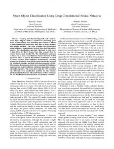
Firstly, we used the BEA Hungarian Spoken Language Database (Gosy, 2012). It is the largest speech database in Hungarian, which contains 260 hours of material produced by 280 speakers (aged between 20 and 90 years), recorded in a sound-proof studio environment. In the present study, we used the conversational speech material, a total of 75 conversations, with an average duration of 16 minutes. The segment boundaries of laughter segments were identified by human transcribers. Our presegmented data contains manually annotated segments, namely 332 laughter and 321 speech segments. Here, we used one-third of the data in the test set and two-thirds in the training set. In the end, we had 240 and 223 segments in the training set, laughter and non-laughter, respectively, while the test set was made up of of 91 laughter and 97 non-laughter segments. The distribution of segment lengths in this database can be seen in the upper part of Fig. 3.

−0.5 sigmoid(x) tanh(x) rectifier(x)

−1 −1.5 −2

−1.5

−1

−0.5

0

0.5

1

1.5

2

Fig. 2. The sigmoid, tanh and linear rectifier functions.

40

40

30

30

No. of occurrences

No. of occurrences

The principal advantage of deep rectifier nets is that they can be trained with the standard backpropagation algorithm, without any pre-training. In our previous experiments on phoneme classification (Grósz, Tóth, 2013); Tóth, 2013), they were found to yield phone recognition scores similar to those of sigmoid networks pre-trained with the DBN algorithm on several databases, but their training times were much shorter. Therefore, in the experiments performed in our study, we decided to employ only Deep Rectifier Neural Networks.

laughter speech both

20

10

0 0

0.5

1

1.5


20

10

0 0

2

0.5

1

80

80

70

70

60

60

50

laughter speech both Gamma dist.

40 30 20 10 0 0

1.5

2

Length (sec)

No. of occurrences

No. of occurrences

Length (sec)

50


40 30 20 10

0.5

1

1.5

Length (sec)

2

2.5

3

0 0

0.5

1

1.5

2

2.5

3

Length (sec)

Fig. 3. The distribution of length of segments belonging to the two classes for the BEA (up) and the SSPNet Vocalization (down) corpus, for the training set (left) and the test set (right).



4.2. The SSPNet Vocalization Database The SSPNet Vocalization Corpus (Salamin et al., 2013) consists of 2763 short audio clips extracted from English telephone conversations taken from 120 speakers, containing 2988 laughter and 1158 filler events. In the public annotation, each frame fell into one of three classes of “laughter”, “filler” and “garbage” (denoting both non-filler, non-laughter speech and silence). Here, we followed the standard train-test division of the database applied in several studies, e.g. (Brueckner, Schuller, 2013; Gosztolya, 2015b); Gosztolya et al., 2013; Gupta et al., 2013; Schuller et al., 2013), adding the development set to the training set. To mirror the set-up of the BEA laughter corpus, we used all the laughter events, and sought to extract similar-sized excerpts of the utterances to provide nonlaughter segments. To do this, we fitted a gamma disćs, 1955) over the length of laughter tribution (Luka segments, and segments containing non-laughter were extracted from the utterances based on this distribution. (Note that, of course, the extracted segments might contain filler events along with silent parts.) We followed this procedure for both the training and test sets, with the exception that the excerpts from the test set were extracted using the probability distribution fitted on the training set. Lastly, we discarded all those segments that were shorter than 100 milliseconds, as we considered them too short to be useful in practice. In the end we had 869 and 964 segments in the training set, while the test set consisted of 280 and 310 excerpts, laughter and non-laughter, respectively. The distribution of the segments of the training set for the SSPNet Vocalization corpus and the fitted (and scaled) Gamma distribution can be seen in the lower part of Fig. 3. 4.3. Experimental setup We used our custom neural network implementation, which achieved outstanding results on several datasets, e.g. (Gosztolya et al., 2014; Grósz et al., 2015; Tóth, 2015; Tóth et al., 2015). Following preliminary tests, we opted for three hidden layers, each one containing 256 rectified neurons, and we applied the softmax activation function in the output layer. We utilized the L2 normalization weight regularization technique. We tested three standard and popular feature sets: we calculated the 12 MFCC, 12 PLP and 40 raw Mel-scale filter banks (FBANK); by adding energy as a further (frame-level) feature, and calculating the first and second order derivatives, we had 39, 39 and 123 attributes for the MFCC, PLP and FBANK feature sets, respectively. It is a well-known fact, e.g. (Blomberg, Elenius, ćs, Tóth, 1992; Bourlard, Morgan, 1993; Kova 2015) that for frame-level phoneme identification, in-

673

cluding the feature values of the neighbouring frames could actually assist the classification process. It is not surprising that the effectiveness of this simple technique has been demonstrated for laughter identification as well, e.g. (Brueckner, Schuller, 2013). Hence we decided to include such a frame context in our laughter classification experiments. Since the optimal number of neighbours is unknown in advance, and could vary depending on the feature set or even on the database, we tested several values; namely, we tried out a training window of 1, 3, 5, . . . , 21 frames wide (i.e. using 0, 1, 2, . . . , 10 neighbouring frames on each side). Instead of using a separate training and development set, we opted for 10-fold cross validation. Since training a neural network is a stochastic procedure due to random weight initialization, we trained five different networks (with different random seed) for each 9-fold training part, resulting in 50 trained networks overall. Then we evaluated them on the remaining fold, and calculated the CV confusion matrix based on the outputs. For the test set we decided to evaluate only five neural networks (with different random seed), since the 9-fold training sets share most of the training data, so training five models on one of these training sets represents all the models quite well. Besides standard accuracy, we also measured precision, recall and F-measure (or F1 -score, being the harmonic mean of precision and recall) for the laughter class. Of course, as the class distribution was quite balanced, the F1 score could be expected to fall quite close to the accuracy score. Apart from performing frame-level classification, we also performed classification of whole segments. We did this in a straightforward way: we multiplied the frame-level posterior scores for both classes, and chose the class for which this score was the highest. This is a viable way of aggregating frame-level likelihoods, especially as Deep Neural Networks are known to provide fairly precise posterior estimation scores.

5. Results The results obtained on the BEA dataset can be seen in Fig. 4, and some notable cases are listed in Table 1. It is clear that using the feature vectors of the neighbouring frames generally helps the classifier, although the optimal value depends on the feature set and evaluation metric (i.e. accuracy or F-measure) used. For MFCC the best results were obtained by using 9–11 frame vectors (4–5 neighbours on each side), while for PLP we had to use a 7–11 frame wide window (3–5 neighbours) to get the highest accuracy scores. Another interesting observation is that the segmentlevel scores are much higher than the frame-level ones. This is expected, though, since it is enough to correctly identify the majority of the frames of a segment to clas-


674


90

100 97.5

80 75 70 Accuracy (CV) F (CV) 1

65 60

Segment accuracy (%)

Frame accuracy (%)

85

1

3

5

7

9

11

13

15

17

92.5 90 Accuracy (CV) F (CV) 1

87.5

Accuracy (test) F (test) 1

95


85

19

21

1

3

5

No. of neighbouring frames



Frame accuracy (%)

13

15

17

1

3

5

7

9

11

13

15

17

Accuracy (test) F1 (test)

95 92.5 90

85

19

21

1

3

5


95

97.5


75


5

7

9

11

13

15

17


100

3

7

9

11

13

15

17

19

21


100

1

21

87.5


19

Accuracy (CV) F1 (CV)

97.5

65

Frame accuracy (%)

11

100

85

70

9


90

60

7

95 92.5 90 Accuracy (CV) F (CV) 1

87.5


85

19

21


1

3

5

7

9

11

13

15

17

19

21


Fig. 4. The frame-level (left) and segment-level (right) accuracy scores and F1 scores obtained by applying the MFCC (upper row), PLP (middle row) and FBANK (lower row) feature sets on the BEA dataset.

sify it correctly. We should also mention that framelevel optimality and segment-level optimality are not always achieved under the same circumstances. For instance, for MFCC, frame-level optimum is achieved by training on 11 frames, while the best segment-level values were obtained with 9 frames. The results obtained by using the FBANK feature set are pretty surprising. We observe that a practically perfect classification was achieved when we used no neighbours at all; and using additional frames only makes the results worse. We think that this good performance is partly due to the high precision of DNNs, the fact that the FBANK feature set is suitable for this classifier, and that the laughter classification task is relatively simple (e.g. compared to phoneme pos-

terior estimation). Still, this score seems too high to be explained by these phenomena alone. Noting that on this dataset similarly high, although no such exceptional scores were reported recently, e.g. (Neuberger, Beke, 2013b; Neuberger et al., 2014), we think that this high score partially reflects the bias of the dataset. Examining Fig. 3 we see that the distribution of lengths of laughter and non-laughter parts differ significantly, which might be due to the manual extraction of the segments. While we cannot suggest any better method for finding laughter parts, in our opinion the non-laughter segments should be extracted automatically to be as similar to the laughter ones as possible (e.g. following the procedure we used for the SSPNet Vocalization corpus).


675

G. Gosztolya et al. – Laughter Classification Using Deep Rectifier Neural Networks . . . Table 1. Some notable accuracy scores obtained by using the different feature sets and number of neighbours on the BEA dataset. Cross-Validation Type

Feature set MFCC

Frame

PLP FBANK MFCC

Segment

PLP FBANK

Test set

N

Prec.

Recall

F1

Acc.

Prec.

Recall

F1

Acc.

9

78.8%

82.3%

80.5%

87.7%

64.1%

85.8%

73.4%

82.8%

11

79.7%

81.5%

80.6%

87.9%

65.7%

84.9%

74.1%

83.6%

7

80.3%

81.4%

80.9%

88.1%

65.8%

85.9%

74.5%

83.7%

9

80.6%

81.9%

81.3%

88.3%

65.1%

86.7%

74.4%

83.4%

1

99.1%

99.8%

99.5%

99.7%

97.6%

99.3%

98.4%

99.1%

9

98.0%

89.1%

93.3%

93.9%

97.5%

95.5%

96.5%

96.4%

11

98.2%

89.1%

93.4%

94.0%

97.4%

93.8%

95.6%

95.5%

7

98.9%

88.9%

93.6%

94.2%

95.0%

97.1%

96.0%

95.9%

9

98.7%

88.3%

93.2%

93.8%

94.4%

97.3%

95.8%

95.6%

1

100.0%

100.0%

100.0%

100.0%

100.0%

100.0%

100.0%

100.0%

The results obtained on the SSPNet Vocalization corpus can be seen in Fig. 5; and some noteworthy cases are listed in Table 2. Firstly, we can see that the accuracy scores obtained in cross-validation mode tend to be higher than those of the test set. While for the frame-level values this was the case for the BEA dataset as well, there the segment-level scores were quite similar to each other, or the values of the test set were even higher. Here, however, we can see that the segment-level values for the test set are 4−5% lower than those for the cross-validation setup, which is a clear sign of overfitting. This is especially in-

triguing as this dataset is much larger than the first one, and we used the same neural network structure for both databases. Another observation is that by increasing the number of neighbouring frame vectors used, the frame-level accuracy scores keep increasing. Segment-level scores, however, have their optimum between 7 and 13 frames, and adding the feature vectors of more neighbouring frames makes the accuracy scores drop (although the differences are probably not significant). Laughter is a social signal that can be expected to be quite language-independent. Therefore it would

Table 2. Some notable accuracy scores obtained by using the different feature sets and number of neighbours on the SSPNet Vocalization dataset. Cross-Validation Type

Feature set MFCC

Frame

PLP

FBANK

MFCC

Segment

PLP

FBANK

Test set

N

Prec.

Recall

F1

Acc.

Prec.

Recall

F1

Acc.

7

83.1%

87.2%

85.1%

84.0%

80.9%

87.3%

84.0%

81.8%

11

83.5%

87.5%

85.5%

84.4%

81.5%

88.6%

84.9%

82.8%

21

84.4%

87.9%

86.1%

85.2%

82.5%

88.7%

85.5%

83.6%

11

83.5%

87.6%

85.5%

84.5%

81.6%

87.8%

84.6%

82.5%

17

84.0%

88.1%

86.0%

85.0%

82.4%

88.3%

85.3%

83.3%

21

84.5%

87.8%

86.1%

85.2%

82.7%

88.3%

85.4%

83.6%

13

84.4%

89.3%

86.7%

85.7%

81.8%

89.7%

85.6%

83.5%

15

84.6%

89.4%

86.9%

85.9%

81.9%

90.0%

85.8%

83.7%

19

85.2%

89.5%

87.3%

86.3%

82.2%

89.9%

85.9%

83.9%

7

95.8%

94.0%

94.9%

94.8%

88.2%

92.0%

90.1%

89.4%

11

96.1%

93.7%

94.9%

94.7%

88.0%

93.3%

90.6%

89.8%

21

95.8%

94.0%

94.9%

94.7%

87.4%

92.3%

89.8%

89.0%

11

95.6%

94.0%

94.8%

94.6%

88.1%

92.8%

90.4%

89.7%

17

95.9%

94.0%

95.0%

94.8%

88.3%

92.5%

90.3%

89.6%

21

95.9%

93.6%

94.7%

94.6%

88.1%

91.8%

89.9%

89.2%

13

96.0%

94.5%

95.3%

95.1%

87.4%

94.5%

90.8%

89.9%

15

96.0%

94.7%

95.3%

95.2%

87.3%

94.1%

90.6%

89.7%

19

96.5%

94.1%

95.3%

95.1%

87.3%

93.4%

90.2%

89.4%


676


90

97.5

85

80 Accuracy (CV) F (CV)


Frame accuracy (%)

95

1

1

1

3

5

7

9

11

13

15

17

90 87.5 Accuracy (CV) F (CV) 1

85


92.5


82.5

19

21

1

3

5


7

9

11

13

15

17

19

21


90

97.5

85

80 Accuracy (CV) F (CV)


Frame accuracy (%)

95

1

1

1

3

5

7

9

11

13

15

17

90 87.5 Accuracy (CV) F (CV) 1

85


92.5


82.5

19

21

1

3

5


7

9

11

13

15

17

19

21


90

97.5

85

80 Accuracy (CV) F (CV) 1


75 1

3

5

7

9

11

13

15

17


Frame accuracy (%)

95 92.5 90 87.5 Accuracy (CV) F (CV) 1

85


82.5

19

21


1

3

5

7

9

11

13

15

17

19

21


Fig. 5. The frame-level (left) and segment-level (right) accuracy scores and F1 scores obtained by applying the MFCC (upper row), PLP (middle row) and FBANK (lower row) feature sets on the SSPNet Vocalization dataset.

be reasonable (and also very interesting) to find out how classifier models trained on one language perform when evaluated on utterances taken from another language. Unfortunately, the recording conditions of the two datasets used in this study differ to such an extent that all our efforts to train on one database and evaluate on the other resulted in very poor accuracy values. Since the BEA database was recorded in a sound-proof, studio-like environment with a studio microphone, while the English one contains mobile phone conversations, it is not that surprising. However, we were still able to identify a language-independent aspect of laughter which could be detected on these two datasets; now we will examine this phenomenon more closely.

6. Feature selection for laughter classification In our experiments we found that, out of the three feature sets tested, the “FBANK” performed best for both databases. In fact, it performed exceptionally well for the BEA dataset. Recall that this feature set consists of features that represent narrow frequency bands and it is very unlikely that all frequency bands have an equal role in the identification of laughter, or even that all of them are necessary. Owing to this, we will next try to select the features which are essential for high-accuracy laughter detection. In the literature we can find a huge variety of feature selection methods, e.g. (Brendel et al., 2010; Busso et al., 2013; Chandrashekar, Sahin, 2014;


677


the corresponding input features. Naturally, as a negative weight can also reflect the degree of importance, we decided to sum up the squared weights for all input neurons (ignoring the bias values). We did this for all the models trained when no neighbouring frame vectors were used, and then, similar to the previous case, we sorted the resulting values in descending order. 6.1. Results Figure 6 shows the frame-level (left) and segmentlevel (right) accuracy scores obtained when using the top-ranked subset of features, when following correlation-based (up) and DNN-based (down) feature ordering on the BEA database. Overall it is clear that a surprisingly compact feature subset is sufficient to provide optimal or near-optimal accuracy scores on both the development and test sets: by using only 28 and 15 features (correlation-based and DNN-based feature ordering, respectively) instead of all the 123 attributes, we were able to reproduce the perfect segment classification, and the frame-level scores dropped by just 1%. The corresponding values obtained on the SSPNet Vocalization corpus are displayed in Fig. 7. The relatively large gap between the scores obtained by using cross-validation and on the test set shows the amount of model overfitting, which was observed previously. The convergence of the feature selection method is also much slower (notice that the horizontal scale of

100

100

98

99


Frame accuracy (%)

Gosztolya, 2015a). However, to test the efficiency of a feature subset, we have to train and evaluate several deep neural networks, which is a time-consuming process. Therefore we opted for a greedy procedure, for which we first sorted the features according to their potential usability. Then, for the nth step, we used the first n features (following the feature ordering) to train our DNNs; then we evaluated them and noted their performance both in the cross-validation setup and on the test set. Obtaining a good feature ordering for the above procedure is not trivial, and it could be carried out in several ways. Here, we applied two ordering strategies. As we have two classes (i.e. laughter and nonlaughter), calculating the correlation of each feature with the frame-level class labels is fairly straightforward. As a negative correlation could also mean that the given feature is useful for laughter detection, we sorted the features according to the absolute value of their correlation score, and in descending order (so as to have higher-correlated features examined first). Another strategy we applied is based on the observation that the lower layers of a deep neural network are responsible for low-level feature extraction, while the higher layers perform more abstract and more taskdependent functions. Since the neurons in the input layer of a DNN correspond to the input features, the connections between the input neurons and those of the first hidden layer might reflect the importance of


90

1

5

10

15

20

25

30

35

40

97 96 Accuracy (CV) F (CV) 1

95

Accuracy (test) F (test)

88

98


94 45

50

5

10

15

100

100

98

99


90

1

88 10

15

20

25

30

No. of features

30

35

40

45

50

35

40


95


25

No. of features


Frame accuracy (%)

No. of features

20


94 45

50

5

10

15

20

25

30

35

40

45

50

No. of features

Fig. 6. Frame-level (left) and segment-level (right) accuracy scores got when using just the top-ranked n features on the BEA dataset. The feature rankings were obtained based on correlation scores (up) and using DNN weights (down).



86

96

84

94


Frame accuracy (%)

678


76

1

10

20

30

40

50

60

70

80

Accuracy (test) F1 (test)

92 90 88 86

Accuracy (test) F (test)

74

Accuracy (CV) F1 (CV)

84 90

100

10

20

30

86

96

84

94


76


74 10

20

30

40

50

60

40

50

60

70

80

90

100

No. of features


Frame accuracy (%)

No. of features

70

80


86


84 90

100

No. of features

10

20

30

40

50

60

70

80

90

100

No. of features

Fig. 7. Frame-level (left) and segment-level (right) accuracy scores got when using just the top-ranked n features for the SSPNet Vocalization dataset. The feature rankings were obtained based on correlation scores (up) and using DNN weights (down).

Figs. 6 and 7 differ): although relatively good accuracy scores can be achieved by using about 40 and 15 attributes (correlation-based and DNN-based feature ordering, respectively), a further 2-3% can be gained by utilizing more features. Because of this, we selected two feature subsets for both ordering strategies: the first had 40 and 15, while the second contained 89 and 68 features, correlation-based and DNN-based ordering, respectively. The reason why the DNN-based feature ordering worked better than the correlation-based one is probably that, although correlation is able to characterize the importance of a given feature for the actual twoclass task quite well, it is suboptimal for feature sets. Features containing similar information are likely to get similar correlation values, so a feature set containing highly-correlated features can expected to be quite a redundant one. As the FBANK feature set consists of overlapping spectral bands, it is not surprising that the neighbouring filter bank features tend to be similar to each other. This results in an unnecessarily large feature subset when we seek optimal performance. 6.2. Feature Subset cross-corpus evaluation Next, we will examine how the optimal feature subsets selected above work when they are used for the

other database. That is, we will take a feature set found optimal or close-to-optimal on the BEA corpus, and train and evaluate our DNNs on the SSPNet Vocalization dataset using just this feature subset; then we will repeat this process the other way around with these two databases. This way, we can test the corpus-independence of the selected feature subsets. Recall that we selected 2 feature sets based on the BEA database and 4 sets based on the SSPNet Vocalization corpus, which, along with the full feature set, results in seven cases in total for both datasets. The resulting accuracy scores can be seen in tables 3 and 4. For the BEA database we were able to achieve a perfect segment classification by using practically any feature subset; the only exception was the smaller subset obtained by relying on the DNN weights of the SSPNet Vocalization dataset. It is not that surprising, though, since this is a very compact feature set, and even on the SSPNet corpus it lagged behind the full feature set by 2−3% in terms of segment-level accuracy scores. Note that this configuration resulted in much lower frame-level accuracy scores (6−15%) on the BEA database, while the segment-level scores dropped only slightly. The results on the SSPNet Vocalization database reveal the differences between the feature selection techniques in more detail, as here we could not achieve


679

G. Gosztolya et al. – Laughter Classification Using Deep Rectifier Neural Networks . . . Table 3. The number of features used and the accuracy scores obtained by feature selection and using no neighbours on the BEA dataset. Training set Cross-Validation Type

Frame

Segment

Test set

Feature set

#F

Prec.

Recall

F1

Acc.

Prec.

Recall

F1

Acc.

Corr. (BEA)

29

96.9%

99.4%

98.1%

98.8%

94.3%

98.0%

96.5%

98.0%

DNN (BEA)

15

97.0%

99.4%

98.2%

98.9%

95.2%

98.7%

96.9%

98.3%

Corr. (SSPNet)

40

97.1%

99.5%

98.3%

98.9%

92.9%

99.0%

95.9%

97.6%

Corr. (SSPNet)

89

98.2%

99.8%

99.0%

99.4%

94.8%

99.2%

96.9%

98.3%

DNN (SSPNet)

15

85.6%

92.3%

88.8%

92.8%

74.2%

89.7%

81.2%

88.5%

DNN (SSPNet)

68

99.1%

99.9%

99.5%

99.7%

96.4%

99.3%

97.8%

98.8%

Full

123

99.1%

99.8%

99.5%

99.7%

97.6%

99.3%

98.4%

99.1%

Corr. (BEA)

29

100.0%

100.0%

100.0%

100.0%

100.0%

100.0%

100.0%

100.0%

DNN (BEA)

15

100.0%

100.0%

100.0%

100.0%

100.0%

100.0%

100.0%

100.0%

Corr. (SSPNet)

40

100.0%

100.0%

100.0%

100.0%

100.0%

100.0%

100.0%

100.0%

Corr. (SSPNet)

89

100.0%

100.0%

100.0%

100.0%

100.0%

100.0%

100.0%

100.0%

DNN (SSPNet)

15

98.3%

100.0%

99.2%

99.2%

96.7%

97.5%

97.1%

97.0%

DNN (SSPNet)

68

100.0%

100.0%

100.0%

100.0%

100.0%

100.0%

100.0%

100.0%

Full

123

100.0%

100.0%

100.0%

100.0%

100.0%

100.0%

100.0%

100.0%

Table 4. The number of features used and the accuracy scores obtained by feature selection and using no neighbours on the SSPNet Vocalization dataset. Training set Cross-Validation Type

Frame

Segment

Test set

Feature set

#F

Prec.

Recall

F1

Acc.

Prec.

Recall

F1

Acc.

Corr. (SSPNet)

40

78.0%

85.9%

81.8%

80.0%

73.6%

86.6%

79.6%

75.8%

Corr. (SSPNet)

89

82.3%

86.7%

84.4%

83.3%

76.6%

88.6%

82.2%

79.0%

DNN (SSPNet)

15

78.8%

82.3%

80.5%

79.2%

75.1%

84.7%

79.6%

76.3%

DNN (SSPNet)

68

82.9%

86.3%

84.6%

83.5%

77.2%

88.6%

82.5%

79.5%

Corr. (BEA)

29

76.7%

83.5%

79.9%

78.1%

73.1%

83.7%

78.0%

74.3%

DNN (BEA)

15

77.5%

82.1%

79.7%

78.1%

74.5%

85.5%

79.7%

76.2%

Full

123

81.9%

86.7%

84.2%

83.0%

78.7%

88.1%

83.2%

80.5%

Corr. (SSPNet)

40

93.4%

94.3%

93.8%

93.6%

82.7%

92.3%

87.2%

85.8%

Corr. (SSPNet)

89

95.5%

94.1%

94.8%

94.6%

84.7%

93.3%

88.8%

87.6%

DNN (SSPNet)

15

93.8%

92.5%

93.2%

92.9%

83.2%

92.2%

87.5%

86.1%

DNN (SSPNet)

68

95.4%

93.4%

94.4%

94.3%

85.0%

94.1%

89.3%

88.1%

Corr. (BEA)

29

91.2%

91.6%

91.4%

91.0%

81.8%

88.0%

84.8%

83.4%

DNN (BEA)

15

91.9%

90.3%

91.1%

90.8%

83.0%

89.8%

86.3%

85.0%

Full

123

95.5%

93.9%

94.7%

94.6%

86.1%

93.7%

89.8%

88.8%

a perfect segment classification. Using the feature subsets selected on the BEA dataset, we got slightly (1– 2%) lower accuracy scores than when we performed feature selection solely on the SSPNet Vocalization corpus. Of course, as this dataset was quite sensitive to the number of features used, and larger feature subsets were selected on it than on the other database, it is not easy to make a fair comparison. Overall, the selected feature subsets seem to be quite robust, as using them on a different dataset did not significantly reduce the accuracy scores.

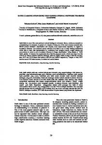
Figure 8 above shows the spectrogram of a laughter segment, its FBANK representation, and the filter bands chosen based on the weights of the DNN for the two datasets. (For the sake of clarity we will show only the first 40 attributes, omitting the first and second order derivatives; if a derivative feature was selected, we highlight the basic frequency band instead.) Surprisingly, quite different attributes were chosen, although specific bands (especially those corresponding to the lower frequencies) of the full spectrum were preferred in both cases. It is quite interesting that when


680


Fig. 8. The spectrogram of a laughter event (upper left), the 40 FBANK features extracted from it (upper right), and the filter bands selected based on the weights of the DNN for the BEA (lower left) and the SSPNet Vocalization (lower right) corpora.

we filtered the features based on the weights of DNNs trained on the BEA database (lower left image), in a region every second filter band was chosen. This is probably because the adjacent filters are redundant to some extent, so every second one encodes enough information to allow high-precision laughter classification. Interestingly, the DNNs were able to detect this phenomenon, and we could extract this information just by examining the weights between the input layer (the filter banks) and the first hidden layer.

7. Conclusions In this work we experimented with detecting laughter events using Deep Rectifier Neural Networks. We carried out our experiments with two databases and utilized three acoustic feature sets. From our results it is seen that DNNs can be effectively applied in this task and they are able to achieve fairly high accuracy scores. We also found that not all frequency regions are required to identify laughter, and that the weights of a trained neural network can be used to find a sufficient feature subset. Furthermore, it seems that these frequency band subsets are quite language-independent, as we were able to carry them over from one database to the other with only a small drop in the overall performance.

8. Acknowledgments This work was supported by the Hungarian Scientific Research Fund (OTKA) 108762. The Titan X graphics card used for this research was donated by the NVIDIA Corporation.

References 1. Bachorowski J.-A., Smoski M.J., Owren M.J. (2001), The acoustic features of human laughter, Journal of the Acoustical Society of America, 110, 3, 1581– 1597. 2. Bickley C., Hunnicutt S. (1992), Acoustic analysis of laughter, [in:] Proceedings of ICSLP, pp. 927–930, Banff, Canada. 3. Blomberg M., Elenius K. (1992), Speech recognition using artificial neural networks and dynamic programming, [in:] Proceedings of Fonetik, p. 57, G¨ oteborg, Sweden. 4. Bourlard H.A., Morgan N. (1993), Connectionist Speech Recognition: A Hybrid Approach, Kluwer Academic, Norwell. 5. Brendel, M., Zaccarelli, R., and Devillers, L. (2010). A quick sequential forward floating feature selection algorithm for emotion detection from speech. [in:] Proceedings of Interspeech, pages 1157–1160, Makuhari, Japan. 6. Brueckner R., Schuller B. (2013), Hierarchical neural networks and enhanced class posteriors for social signal classification, [in:] Proceedings of ASRU, pp. 362–367.



681

7. Bryant G.A., Aktipis C.A. (2014), The animal nature of spontaneous human laughter, Evolution and Human Behavior, 35, 4, 327–335.

¨nther U. (2002), What’s in a laugh? Humour, 23. Gu jokes, and laughter in the conversational corpus of the BNC, Ph.D. thesis, Universit¨ at Freiburg.

8. Busso C., Mariooryad S., Metallinou A., Narayanan S. (2013), Iterative feature normalization scheme for automatic emotion detection from speech, IEEE Transactions on Affective Computing, 4, 4, 386–397.

24. Gupta R., Audhkhasi K., Lee S., Narayanan S.S. (2013), Speech paralinguistic event detection using probabilistic time-series smoothing and masking, [in:] Proceedings of Interspeech, pp. 173–177.

9. Cai R., Lu L., Zhang H.-J., Cai L.-H. (2003), Highlight sound effects detection in audio stream, [in:] Proceedings of ICME, pp. 37–40.

25. Hinton G.E., Osindero S., Teh Y.-W. (2006), A fast learning algorithm for deep belief nets, Neural Computation, 18, 7, 1527–1554.

10. Campbell N. (2007), On the use of nonverbal speech sounds in human communication, [in:] Proceedings of COST Action 2102: Verbal and Nonverbal Communication Behaviours, pp. 117–128, Vietri sul Mare, Italy.

26. Holmes J., Marra M. (2002), Having a laugh at work: How humour contributes to workplace culture, Journal of Pragmatics, 34, 12, 1683–1710.

11. Campbell N., Kashioka H., Ohara R. (2005), No laughing matter, [in:] Proceedings of Interspeech, pp. 465–468, Lisbon, Portugal. 12. Chandrashekar G., Sahin F. (2014), A survey on feature selection methods, Computers & Electrical Engineering, 40, 1, 16–28. 13. Glenn P. (2003), Laughter in interaction, Cambridge University Press, Cambridge, UK. 14. Glorot X., Bordes A., Bengio Y. (2011), Deep sparse rectifier networks, [in:] Proceedings of AISTATS, pp. 315–323. 15. Goldstein J.H., McGhee P.E. (1972), The psychology of humor: Theoretical perspectives and empirical issues, Academic Press, New York, USA. 16. Gósy M. (2012), BEA: A multifunctional Hungarian spoken language database, The Phonetician, 105, 106, 50–61. 17. Gosztolya G. (2015a), Conflict intensity estimation from speech using greedy forward-backward feature selection, [in:] Proceedings of Interspeech, pp. 1339–1343, Dresden, Germany. 18. Gosztolya G. (2015b), On evaluation metrics for social signal detection, [in:] Proceedings of Interspeech, pp. 2504–2508, Dresden, Germany. 19. Gosztolya G., Busa-Fekete R., Tóth L. (2013), Detecting autism, emotions and social signals using AdaBoost, [in:] Proceedings of Interspeech, pp. 220– 224, Lyon, France. 20. Gosztolya G., Grósz T., Busa-Fekete R., Tóth L. (2014), Detecting the intensity of cognitive and physical load using AdaBoost and Deep Rectifier Neural Networks, [in:] Proceedings of Interspeech, pp. 452–456, Singapore. 21. Grósz T., Tóth L. (2013), A comparison of Deep Neural Network training methods for Large Vocabulary Speech Recognition, [in:] Proceedings of TSD, pp. 36– 43, Pilsen, Czech Republic. 22. Grósz T., Busa-Fekete R., Gosztolya G., Tóth L. (2015), Assessing the degree of nativeness and Parkinson’s condition using Gaussian Processes and Deep Rectifier Neural Networks, [in:] Proceedings of Interspeech, pp. 1339–1343.

27. Hudenko W., Stone W., Bachorowski J.-A. (2009), Laughter differs in children with autism: An acoustic analysis of laughs produced by children with and without the disorder, Journal of Autism and Developmental Disorders, 39, 10, 1392–1400. 28. Kennedy L.S., Ellis D.P.W. (2004), Laughter detection in meetings, [in:] Proceedings of the NIST Meeting Recognition Workshop at ICASSP, pp. 118–121, Montreal, Canada. 29. Knox M.T., Mirghafori N. (2007), Automatic laughter detection using neural networks, [in:] Proceedings of Interspeech, pp. 2973–2976, Antwerp, Belgium. 30. Kov´ acs Gy., Tóth L. (2015), Joint optimization of spectro-temporal features and Deep Neural Nets for robust automatic speech recognition, Acta Cybernetica, 22, 1, 117–134. ¨ller F. (2002), LAFCam leveraging 31. Lockerd A., Mu affective feedback camcorder, [in:] Proceedings of CHI EA, pp. 574–575, Minneapolis, MN, USA. ćs E. (1955), A characterization of the Gamma 32. Luka distribution, Annals of Mathematical Statistics, 26, 2, 319–324. 33. Martin R.A. (2007), The psychology of humor: An integrative approach, Elsevier, Amsterdam, NL. 34. Neuberger T., Beke A. (2013a), Automatic laughter detection in Hungarian spontaneous speech using GMM/ANN hybrid method, [in:] Proceedings of SJUSK Conference on Contemporary Speech Habits, pp. 1–13. 35. Neuberger T., Beke A. (2013b), Automatic laughter detection in spontaneous speech using GMM–SVM method, [in:] Proceedings of TSD, pp. 113–120. 36. Neuberger T., Beke A., Gósy M. (2014), Acoustic analysis and automatic detection of laughter in Hungarian spontaneous speech, [in:] Proceedings of ISSP, pp. 281–284. 37. Nwokah E.E., Davies P., Islam A., Hsu H.-C., Fogel A. (1993), Vocal affect in three-year-olds: a quantitative acoustic analysis of child laughter, Journal of the Acoustical Society of America, 94, 6, 3076–3090. ¨nger H., Hauser G., Cappellini A.C., 38. Rothga Guidotti A. (1998), Analysis of laughter and speech sounds in Italian and German students, Naturwissenschaften, 85, 8, 394–402.


682


39. Salamin H., Polychroniou A., Vinciarelli A. (2013), Automatic detection of laughter and fillers in spontaneous mobile phone conversations, [in:] Proceedings of SMC, pp. 4282–4287. 40. Schapire R., Singer Y. (1999), Improved boosting algorithms using confidence-rated predictions, Machine Learning, 37, 3, 297–336. ¨ lkopf B., Platt J., Shawe-Taylor J., 41. Scho Smola A., Williamson R. (2001), Estimating the support of a high-dimensional distribution, Neural Computation, 13, 7, 1443–1471. 42. Schuller B., Steidl S., Batliner A., Vinciarelli A., Scherer K., Ringeval F., Chetouani M., Weninger F., Eyben F., Marchi E., Salamin H., Polychroniou A., Valente F., Kim S. (2013), The Interspeech 2013 Computational Paralinguistics Challenge: Social signals, Conflict, Emotion, Autism, [in:] Proceedings of Interspeech. 43. Suarez M.T., Cu J., Maria M.S. (2012), Building a multimodal laughter database for emotion recognition, [in:] Proceedings of LREC, pp. 2347–2350. 44. Tanaka H., Campbell N. (2011), Acoustic features of four types of laughter in natural conversational speech, [in:] Proceedings of ICPhS, pp. 1958–1961.

45. Tóth L. (2013), Phone recognition with Deep Sparse Rectifier Neural Networks, [in:] Proceedings of ICASSP, pp. 6985–6989. 46. Tóth L. (2015), Phone recognition with hierarchical Convolutional Deep Maxout Networks, EURASIP Journal on Audio, Speech, and Music Processing, 2015, 25, 1–13. 47. Tóth L., Gosztolya G., Vincze V., Hoffmann I., ´ ka ´ski M., Szatlóczki G., Biró E., Zsura F., Pa ´lma ń J. (2015), Automatic detection of Mild CogKa nitive Impairment from spontaneous speech using ASR, [in:] Proceedings of Interspeech, pp. 2694–2698, Dresden, Germany. 48. Truong K.P., van Leeuwen D.A. (2005), Automatic detection of laughter, [in:] Proceedings of Interspeech, pp. 485–488, Lisbon, Portugal. 49. Truong K.P., van Leeuwen D.A. (2007), Automatic discrimination between laughter and speech, Speech Communication, 49, 2, 144–158. 50. Vicsi K., Sztahó D., Kiss G. (2012), Examination of the sensitivity of acoustic-phonetic parameters of speech to depression, [in:] Proceedings of CogInfoCom, pp. 511–515, Kosice, Slovakia.
