Learning-Based Prediction of Visual Attention for Video ... - EPA Lab

IEEE TRANSACTIONS ON IMAGE PROCESSING, VOL. 20, NO. 11, NOVEMBER 2011

1

Learning-Based Prediction of Visual Attention for Video Signals Wen-Fu Lee, Tai-Hsiang Huang, Su-Ling Yeh, and Homer H. Chen, Fellow, IEEE

IE E W E eb P r Ve oo rs f ion

Abstract—Visual attention, which is an important characteristic of human visual system, is a useful clue for image processing and compression applications in the real world. This paper proposes a computational scheme that adopts both low-level and high-level features to predict visual attention from video signal by machine learning. The adoption of low-level features (color, orientation, and motion) is based on the study of visual cells and the adoption of the human face as a high-level feature is based on the study of media communications. We show that such a scheme is more robust than those using purely single low- or high-level features. Unlike conventional techniques, our scheme is able to learn the relationship between features and visual attention to avoid perceptual mismatch between the estimated salience and the actual human fixation. We also show that selecting the representative training samples according to the fixation distribution improves the efficacy of regressive training. Experimental results are shown to demonstrate the advantages of the proposed scheme. Index Terms—Eye tracking experiment, fixation distribution, human visual system, regression, saliency map, visual attention.

I. INTRODUCTION

V

ISUAL attention is an important characteristic of human visual system. It helps our brain to filter out excessive visual information and enables our eyes to focus on particular regions of interest. Supported by the finding that visual attention and eye movement are correlated [1]–[3], eye trackers are used to locate the attended regions in a video. An eye tracker can record various eye movement events, including fixation, saccade, and blink. Among these eye movement events, the fixation is the most indicative of visual attention. The fixation points are usually located in the attended regions; the higher the fixation density, the more attractive the regions. For example, the flower shown in Fig. 1 has the highest fixation density and thus it attracts most attention, whereas the wall and the window shutter behind the flower receive less attention. This example tells us that the

Manuscript received August 11, 2010. revised December 12, 2010; accepted April 03, 2011. This work was supported by Himax Technologies, Inc. The associate editor coordinating the review of this manuscript and approving it for publication was Dr. Alex ChiChung Kot. W.-F. Lee and T.-H. Huang are with the Graduate Institute of Communication Engineering, National Taiwan University, Taipei 10617, Taiwan, R.O.C (e-mail: [email protected], [email protected]). S.-L. Yeh is with the Department of Psychology, National Taiwan University, Taipei 10617, Taiwan, R.O.C (e-mail: [email protected]). H. H. Chen is with the Department of Electrical Engineering, Graduate Institute of Communication Engineering and Graduate Institute of Networking and Multimedia, National Taiwan University, Taipei 10617, Taiwan, R.O.C (e-mail: [email protected]). Color versions of one or more of the figures in this paper are available online at http://ieeexplore.ieee.org. Digital Object Identifier 10.1109/TIP.2011.2144610

Fig. 1. Human fixation data. (a) Original image. (b) Fixation points collected for 5 s of viewing time from 16 subjects.

degree of attention varies from region to region in an image. Many biologically inspired algorithms attempt to mimic this interesting characteristic of human visual systems for various applications, such as image processing [4], [5], video coding [6], and biomedical imaging [7]. For example, by detecting the attended image area, the bit allocation of a video encoder can be improved so that visually more important areas are better preserved in the coding process [6]. Visual attention has been a subject of research in neural science, physiology, psychology, and human vision [8]–[14]. Issues related to the transmission path of a visual signal in the human brain, the visual cells involved in the transmission process, and the change of characteristics of a visual signal caused by the visual cells have been studied. These studies greatly enrich our understanding of the psychophysical aspect of visual attention. Although there is still a long way to fully discover how visual attention is formed in the human brain, existing psychophysical findings can be exploited for visual attention prediction from video signals. A typical visual attention model consists of two parts: extraction of features and fusion of features. The feature extraction takes into account what kind of feature in the image attracts visual attention. It has been found that low-level features such as color, orientation, motion, and flicker attract attention [8]–[12]. These features extracted from the image are further processed by a center-surround mechanism for contrast extraction [15]–[18]. The resulting image, one for each feature, is a feature map, which represents the salience distribution of the feature. The feature maps are then fused to form a saliency map by nonlinear fusion [16], linear fusion with equal weight [17], [18], or linear fusion with dynamic weight [19]–[23]. While the nonlinear fusion approach can better capture the salient region in an image, the other two linear fusion approaches are simpler and more efficient. However, our experiment on eye tracking shows that the salience estimated by a visual attention model using purely low-level features do not always match with human fixations.

1057-7149/$26.00 © 2011 IEEE



2

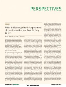
Fig. 2. Mismatch between the actual human fixation and the estimated salience based on low-level features [18]. (a) Original image. (b) Human fixation points overlaid on the estimated saliency map, for which the brightness represents the strength of saliency.

Fig. 3. Eye tracking system. (a) Setup of the eye tracking experiment. (b) Chinand-forehead rest. (c) Nine-point calibration pattern.

II. FIXATION DATA COLLECTION

We find that such a model fails when high-level features such as face and text appear in a video. One such example is shown in the top row of Fig. 2. Since high-level features are common to general video sequences, an attention model using both low-level and high-level features is needed. In addition, even if high-level features do not appear in a sequence, an attention model based on low-level features alone may not always work well. An example is shown in the bottom row of Fig. 2, where the flower has the highest fixation density, but it is not the most salient region despite its high color contrast. This problem is due to improper weight assignment in the feature fusion process. The contributions of this paper are as follows. First, it predicts visual attention from video signal using both low-level and high-level features. Specifically, the proposed scheme uses three low-level features (color, orientation, and motion) and one high-level feature (face). These low-level features are relevant to visual attention [8]–[10], [12], while the face feature conveys information such as happiness or anger that attracts visual attention in social interactions [24], [25]. Experimental results show that this approach is more robust than those that use purely single level features. Second, we develop a computational scheme for visual attention prediction based on machine learning. While previous approaches generate the saliency map by feature fusion explicitly, our approach finds the relationship between the fixation density and the four features by regression. Along with this scheme, novel fixation density estimation and training sample selection techniques are developed that enable the regression model to effectively characterize the relationship between the four features and visual attention in the machine learning process. The remainder of the paper is organized as follows. Section II describes the eye tracking experiment for fixation data collection and the analysis of the resulting fixation distribution. Section III presents the proposed learning-based approach to visual attention prediction. The experimental results are given in Section IV. Finally, the concluding remarks are drawn in Section V.

The fixation data for training a regressor were collected by using an eye tracking system that recorded the fixation of a subject. An experiment was conducted for each subject in a freeviewing fashion without any prior training to ensure that the collected fixation data are stimulus-driven rather than goal-driven. This is important as it allows effective learning of the relationship between features and visual attention for the regressor. Note that, even with the free-viewing fashion, it is impossible to rule out definitively the top-down influences. A. Eye Tracking Apparatus

As shown in Fig. 3(a), the eye tracking system consists of an infrared camera, a host PC, a display PC, and a chin-andforehead rest. The infrared camera tracks the eye movement of the subject, the host PC collects human fixation data, and the display PC presents the stimuli to the subject. The visual angle accuracy of the system is 0.5 . The infrared camera captures 1000 video frames per second. The output video rate on the display PC is 30 frames per second. B. Subjects

Eighteen subjects (nine men and nine women) with different backgrounds and at ages ranging from 20 to 44 were invited to participate in the eye tracking experiment. Every subject had normal or corrected-to-normal vision and no prior experience in the kind of experiment and test content described here. The head of a subject is supported by a chin-and-forehead rest [see Fig. 3(b)] in the experiment. C. Stimuli

We selected 17 video sequences at CIF resolution (352 288 pixels) as the test data of the experiment (see Fig. 4). These sequences (30 Hz, 5.0–10.0 s) were selected because they were conveniently accessible on the Internet. They covered indoor/outdoor scenes, still/moving objects and nature/artificial

LEE et al.: LEARNING-BASED PREDICTION OF VISUAL ATTENTION FOR VIDEO SIGNALS

3


Fig. 5. Configuration of the test data in each trial of the eye tracking experiment. The 17 test sequences are displayed in a random order. The white noise map, which is inserted at the beginning of each test sequence, is displayed for 500 ms before the test sequence starts to play. The combined sequence is displayed at 30 Hz.

TABLE I RESULTS OF THE EYE TRACKING EXPERIMENT

Fig. 4. Test video sequences. (a) Coastguard. (b) Foreman. (c) Highway. (d) MadCyclistL. (e) Paris. (f) Silent. (g) Stefan. (h) Tempete. (i) Weather. (j) Deadline. (k) News. (l) Sign Irene. (m) Students. (n) Waterfall. (o) Vectra. (p) Ice. (q) Soccer.

objects. These test sequences were resized to 640 when displayed to the subjects.

480 pixels

D. Experimental Setup

The viewing distance between the subject and the display PC was four times the height of the display screen, as shown in Fig. 3(a). The horizontal and vertical visual angles of the display are 18.92 and 14.25 , respectively. As the subject’s chin and head were well seated on the chin-and-forehead rest, a camera calibration process started to map the gaze of the subject to the fixation samples on the display PC. In the calibration process, the subject sequentially fixated, one at a time, through a nine-point pattern [see Fig. 3(c)] to complete the construction of a mapping function. Such a pattern ensures that the camera tracks the whole vision of the subject. Then, the subject was instructed to confine the vision within the display screen. This instruction helped prevent the subject from navigating the surrounding environment. Two trials were allowed for each subject. In each trial, the 17 test sequences were displayed in a random order, as shown in Fig. 5. Conventionally, the subjects are asked to fixate at a center point on the screen so that they can keep concentrating on the experiment before the stimulus onsets. However, such an approach may produce a side effect called central bias, resulting in unreliable fixation data. Instead, we used a white noise map as shown in Fig. 5 in our experiment because it could attract the attention of the subject and avoid the central bias problem. In

addition, the white noise map served as an eraser that clears the previous sequence from the subject’s memory. Note that we do not reject any subject in the experiment. E. Results

The results of the eye tracking experiment are shown in Table I. As we can see, there are only two to three fixations per second for a subject. This means that a subject can do at most one fixation per frame. Thus, it is impossible to understand visual attention to video content by observing the fixation distribution of only one subject. To overcome the problem, we add the fixation points of all the subjects to an empty map for each frame to generate a “fixation map.” A region is more attractive (and hence more salient) if it has a higher fixation density. Fig. 6 shows several examples of fixation map. III. PROPOSED LEARNING-BASED APPROACH

The block diagram of the proposed computational scheme for visual attention prediction from video signal is shown in



4

Fig. 8. Fixation density estimation. (a) Original image. (b) Fixation map. (c) The 3-D view of the fixation density map. (d) Fixation density map.

Fig. 6. Results of eye tracking for three test sequences. The top row is the sampled video frames of a test sequence. The bottom row is the corresponding fixation maps.

th fixation point. These fixation points are interpolated by a Gaussian function to generate a fixation density map

(1) where and , respectively, denote the horizontal and vertical is the standard deviation of the positions of a pixel and Gaussian funciton. We determine the value of according to the visual angle accuracy of the eye tracking system. More precisely (2)

Fig. 7. Schematic diagram of salience estimation.

Fig. 7. The empirical fixation data collected by an eye tracker from human subjects are used as the ground truth. The regressor training is applied to determine the regression model that relates the color, motion, orientation and face features to the fixation density based on the ground truth. The regressor thus obtained is used to predict the fixation density and hence the salience of a test video sequence. Details of the scheme are described here. A. Fixation Density Map

The attention of an image region is measured by fixation density. In other words, the salience of an image or a video frame is represented by a fixation density map. The fixation map generated in the data collection process for each video frame of a training sequence is a set of discrete fixation points , where is the total number of fixis the location of the ation points found in a frame and

where is the viewing distance between the subject and the display. We can see from (1) that the fixation density is obtained by taking the Gaussian weighted average of the fixation values. In this way, the value of each fixation pixel is propagated to its neighboring fixation pixels. Therefore, a pixel in a densely populated fixation area is more attractive than a pixel in a sparsely populated fixation area. For the same reason, a region is more attractive if it is brighter on the fixation density map, as shown in Fig. 8(d). B. Feature Extraction

Feature extraction is applied to both training and testing sequences. For each video frame, we generate three low-level feature maps based on the color, orientation and motion information of the video frame, and one high-level feature map based on the face information. 1) Color: The construction of the color map consists of four key steps. First, each frame is converted to the opponent color space developed by Krauskopf et al. [26] so that each video frame can be analyzed in a way similar to how the visual signals are processed by the cone cells of the retina [27]. The primary color components in this color space are achromatic (white–black), chromatic (red–green) and chromatic (blue–yellow). Second, the three primary components are decomposed into a total of 27 subbands, 17 for component and


is the histogram of , is the bin number, is the where is the probability total number of the histogram bins, and of each bin. A low entropy value means that most salience values fall in a small number of bins. In this case, salience distribution is relatively uniform and hence is less conspicuous. Finally, , , the saliency map is obtained by taking the average of . and 2) Motion: In the cortex of the human brain, the neuron cells are found to respond to the motion contrast [9]. The larger the motion contrast, the stronger the response of the neural cells. Based on this finding, we construct a motion map from the relbetween two successive frames of a sequence. ative motion Specifically, a frame is divided into 8 8 blocks, and the block matching approach [30] is applied to estimate the local motion of each block. Then, to take the camera motion into account, we remove the camera-induced motion from the local motion to obtain the relative motion of a block


Fig. 9. Spatial frequency decomposition of the achromatic component of a color signal. From the inner crown to the outmost crown, the frequencies are partitioned into one, four, six, and six subbands, respectively [28].

five for each of and , according to a study on the computation of visual bandwidths [28]. Let denote a primary com. Each subband of the component ponent, of a video frame is defined by

(3)

where is the subband image, is its Fourier transform, and is the index of the crowns (see Fig. 9), given by if if

(4)

where is the orientation index and denotes inverse Fourier transform. Each subband is regarded as the equivalent of the neural image transmitted to the receptive field of a particular population of cortical cells. These cells are tuned to a range of radial spatial frequencies and a particular orientation [28]. Third, each subband image, at its full resolution after decomposition, is convolved with a difference of Gaussian function [29] to compute the color contrast of the subband image. Here, two Gaussian functions with standard deviation 0.573 and 0.6 are used in the modeling of the center-surround mechanism of the cortical cells. By combining the color contrast of each subband, of the component is obtained. the salience distribution is multiplied by a weighting factor as follows: Fourth, (5)

where nent,

5

is the updated salience distribution of the compois the entropy of , and is the maximum of . The choice of the weight is proportional to the entropy of the salience. By definition, we have

(6) (7)

(8)

and are the local motion and the camera-induced where motion, respectively, of a block. Here, the local motion of the still background is caused by the motion of the camera. If the camera is still, the local motions of background blocks are zero. In its simplest form, the simple block matching algorithm generates translational motion estimate, which is a good approximation in many applications, although a more sophisticated motion model can be applied. Once the local motions of all the image blocks are obtained, we use the RANSAC method [31] to extract camera motion from local motion. The affine transform is adopted to represent the camera motion of a block defined by

(9)

is the camera motion of the block, is where the location of the block, and ’s are the parameters of the affine transform. The RANSAC method is implemented in two steps. First, we randomly select three blocks from all the image blocks to calculate the affine transform and take the remaining blocks to validate the result, assuming that the local motions of the three selected blocks are induced by the camera motion. Here, the locations and the local motions of the three selected blocks are used to calculate the six parameters of the affine transform. Second, the resulting affine transform is used to check whether the local motion of each remaining block is induced by the camera motion. This involves measuring the similarity between the local motion of each block and the camera motion calculated by (9) using the affine transform obtained in the first step. If the similarity is high, we consider the local motion of the block an inlier. The final affine transform corresponds to the one with the most inliers. Then, the final camera motion of each block is calculated by using the final affine transform and the relative motion of each block is obtained by (8). The motion map of a video frame contains the magnitude of the relative motion of each block in the video frame.

6



Fig. 10. Similar video frames in the sequence may have different fixation distributions. (a) Original image. (b) Fixation map. (c) Fixation density map. The fixation map can change over time. The top frame: the 8th frame of Waterfall sequence; the bottom frame: the 90th frame.

3) Orientation: The luminance layer of each video frame is filtered in parallel by two low-pass Gaussian filters with different standard deviations. Then the orientation model developed by Itti et al. [18] is applied to extract the local orientation of each pixel of the two low-pass filtered images. The results are two local orientation images. The oriented Gabor filter used in this model is the product of a 2-D Gaussian filter and an oriented cosine grating. This filter is adopted because it approximates the response of orientation-selective neurons in primary visual cortex [32]. The contrast of orientation, which is obtained by computing the difference of the two local orientation images, forms the orientation map. 4) Face: The relationship between human face and attention has been studied in psychology [24], [25]. It is found that even “unexpressive” (or neutral) faces convey emotions and attract visual attention. Thus, human face is selected as a feature in the proposed scheme. The face detector developed by Nilsson et al. [33] is adopted because it is efficient and is able to cope with illumination variation. C. Selection of Training Samples

A training sample consists of the fixation density value and the four feature values of a pixel. Thus, a quintuplet is formed. Given a number of training sequences, there are obviously more training samples than we need for regressor training. A selection process is needed to screen the training samples. 1) Frame Selection: From each video sequence, we select a single frame that has the most representative visual attention of the video sequence. The degree of representativeness is determined by the density of the corresponding fixation points. As we can see, the top fixation density map in Fig. 10 concentrates near the center region, whereas the bottom one spreads across the image. The distribution of the fixation points varies from frame to frame because, as time goes by, each subject has different regions of interest when watching the sequence. However, the subjects will look at more or less the same region of a video frame if it is the most attractive region. In other words, the region will have dense fixation points. Since the spatial fixation distribution of a video frame reflects the degree of attention of the video frame, we find the centroid of the fixation points for each

Fig. 11. Training sample selection (a) The original image (b) the fixation density map (c) the histogram of the block-wise average fixation density values and (d) the selected sample pixels overlaid on the fixation density map.

video frame of a sequence and calculate the mean of the distance between each fixation point and the centroid. The frame with the smallest mean is selected as the representative frame of the sequence. One may select more than one representative frame from each sequence. In the current scheme, since there is no scene change in the selected video sequences, we only select one representative frame. 2) Pixel Selection: Only a relatively small number of pixels are selected from each representative frame as the sample pixels. Once the sample pixels are selected, the training samples are obtained by composing the quintuplets associated with the sample pixels. In our scheme, the sample pixels are selected from the fixation density map according to two guidelines. First, pixels are selected from different parts of the fixation density map to achieve diversity. Second, because most pixels of a fixation density have low values, more pixels are selected from the dense areas of the fixation density map to make the fixation density values uniformly distributed and avoid the regressor training from prediction bias. Under the above guidelines, the selection procedure starts with the partition of a fixation density map into 32 32 blocks, as shown in Fig. 11(b). The average fixation of each block is calculated, where and , density value respectively, denote the horizontal and vertical positions of a , of the average fixblock. Then, the histogram, denoted by ation density values of the blocks is built, as shown in Fig. 11(c). represents the fixation denSpecifically, each bin width of sity interval and each bin height represents the number of blocks whose average density values fall in the interval. According to pixels are selected from the the second guideline, exactly pixels blocks in each bin. Then, as shown in Fig. 11(d), are randomly selected from each block as (10)

where is an operator that returns the index of the bin into which falls. The result is that each interval contains the fixation density values of exactly training samples. Note that, if , the number the value of is not divisible by the number


of selected pixels for the th bin is smaller than is sulting difference between and

. The re-

7

TABLE II PERFORMANCE OF THE REGRESSOR TRAINING

(11) To select more pixels, we randomly select blocks from the and then select one pixel from blocks in the th bin of each of the blocks. In this way, the fixation density values of the resulting training samples are uniformly distributed. D. Regressor Training and Salience Estimation


After the training samples are obtained, the regressor is trained to learn the relationship between the fixation density and the features of the training samples. The popular learning algorithm—support vector regression (SVR)—is adopted for this training process, which mainly consists of two steps. In the first step, the training samples are normalized to make each feature of the training samples have zero mean and unit variance. Note that the same normalization parameters are used for the test samples. In our approach, the radial basis function (RBF) is used to model the relationship between the features and the fixation density because it generally has fewer parameters and better performance than other kernels [34]. In the second step, we determine the parameters for the RBF by grid search [34], which first uses a coarse grid to find the candidate parameter values and then a finer grid in the neighborhood of the candidates for refinement. The search continues until a predefined accuracy is reached. To recap, the regressor training uses the empirical fixation data collected by the eye tracker to construct a regression model that relates the four features (i.e., color, motion, orientation, and face) to the fixation density. In this process, the fixation data of the subjects are collected for the training sequences. On the other hand, in the salience estimation process, the regressor obtained in the training process is used to predict the fixation density (and, hence, the salience) for a test video sequence based on the color, motion, orientation and face features extracted from the test sequence. The same feature extraction algorithm for regressor training is used here in the saliency estimation process. The decision of the best regressor is made by using the leaveone-out (LOO) cross-validation technique, which is known to provide an almost unbiased estimate of the generalization error even when a small dataset is available [35]. As its name suggests, the LOO technique entails partitioning the dataset: One sequence is selected as the test set and the remainder as the training set. In our implementation, the dataset consists of the 17 video sequences described in Section II-C. The LOO procedure is repeated (17 times in our implementation) until every video sequence has been served as a test set. A regressor is generated in each iteration. At the end of the procedure, the one that leads to the fixation density data that are closest to the ground truth is considered the best regressor. IV. EXPERIMENTAL RESULTS

We perform both objective and subjective evaluations of the proposed learning-based approach (LBA) to visual attention prediction. Specifically, we compare: 1) the effect of the

combination of low-level and high-level features on visual attention prediction against that of the single level features and 2) the performance of LBA against that of a well-known linear fusion. In the first comparison, the LBA is implemented with four different feature combinations: 1) all color, orientation, motion, and face features; 2) only color, orientation, and motion features; 3) only color and orientation features; and 4) only face feature. These four feature combinations are denoted COMF, COM, CO and F, respectively. In the second comparison, the LBA is compared with Itti’s approach (noted Itti) [18], which is a linear fusion scheme with equal weight. To have the same basis for comparison, Itti’s features are used in the LBA. In our experiment, we select LIBSVM1 to implement the SVR. A. Performance of Regressor Training

The performance of the regressor training is shown in Table II, where the mean squared error is defined as

(12)

where is the total number of training examples, is the ground truth of the fixation density and is the fixation density predicted by the regressor. We can see that the mean squared errors of the proposed learning-based visual attention scheme are consistently small for all test sequences. Our experiment also shows that there is no outlier on the training samples, indicating that the training sample selection described in Section III-C works effectively. B. Objective Evaluation

Two metrics based on the receiver operating characteristics (ROCs) [17], [36] and the linear correlation coefficient (LCC) [17], [29] are used in the objective evaluation. 1) ROC Analysis: The ROC is used to evaluate how well a saliency map predicts visual attention. The ROC value of a saliency map is obtained as follows. First, the saliency map is 1http://www.csie.ntu.edu.tw/~cjlin/libsvm/



8

Fig. 12. (a) ROC curves for various feature combinations. (b) ROC curves for the LBA and the Itti schemes using the same features.

TABLE III RESULTS OF THE T-TEST FOR ROC CURVES

successively thresholded so that a given percentage of the most salient pixels are retained. Second, for each threshold, we calculate the percentage of fixation points collocated with the retained salient pixels. Plotting the resulting percentage against the threshold yields an ROC curve. Results of the objective evaluation are shown in Fig. 12, where each ROC curve is the average over the 17 testing sequences. The more the ROC curve is near the top left corner of Fig. 12, the better the prediction of visual attention. Note that the dashed line, which is called the chance line, corresponds to the result of a saliency map generated by chance. Fig. 12(a) shows the result of the first comparison. We see that the feature combination COMF leads to better performance than the other feature combinations. Therefore, the combination of both low-level and high-level features is more effective for visual attention prediction. Fig. 12(b) shows the result of the second comparison. We see that the LBA outperforms the Itti scheme. The maximum performance difference is 0.25, which occurs when 30% of the most salient pixels are retained in the thresholded saliency map. Note that all ROC curves in Fig. 12 are above the chance line, indicating that the proposed visual attention modeling scheme performs better than random guess. To statistically measure the dispersion on the ROC curves, a paired-sample t-test [17] is adopted. As shown in Table III, by and large, there is a significant difference (at the level of 0.05) between the feature combination COMF and each of the other feature combinations. Table III also shows a significant difference (at the level of 0.01) between the LBA scheme and the Itti scheme.

2) LCC Analysis: The LCC measures the linear correlation between the saliency map and the fixation density map. It is used to evaluate how close the saliency map is to the fixation density map. Denote the fixation density map by , the saliency map by , and the LCC between and by . Then, by definition [17], we have (13)

where is the covariance between and and and are the standard deviations of and , respectively. The LCC values of the saliency maps for various feature combinations and sequences are shown in Table IV. We see that the average LCC over the 17 testing sequences for COMF is higher than those for the other feature combinations. This shows that, on the average, combining both low- and high-level features is more effective for visual attention prediction than combining the single level features. The paired-sample t-test [17] result also shows that there is a significant difference (at the level of 0.01) between COMF and each of the other feature combinations, indicating that COM and CO, which are purely low-level features, are not as effective as COMF when human faces are present in the sequences (those marked by *). By and large, the feature F, which is a purely high-level feature, is extremely effective for sequences with human faces. The Highway sequence, which contains no human face, receives an LCC value higher than expectation. A careful examination of the results reveals that false faces are generated for the sequence because the face detection algorithm is sensitive to noise for images of low lu-


9


TABLE IV COMPARISON OF LINEAR CORRELATION COEFFICIENT VALUES

Fig. 13. LCC value over time for various feature combinations. Each LCC point is the average over the 17 testing sequences.

minance, which is the case for this sequence. A total of 13 video frames with false faces that happen to overlap with the fixation points are found. These frames contribute to the unexpected high LCC value for the sequence.Table IV also shows that the LBA performs consistently better than the Itti scheme for all sequences. Therefore, the LBA is more effective than the equal-weight linear fusion scheme. The t-test also shows a significant difference (at the level of 0.01) between the LBA scheme and the Itti scheme. In addition, the LBA achieves positive values for all sequences, whereas the Itti scheme gives negative LCC values for three sequences. Therefore, the feature fusion algorithm has a significant impact on the accuracy of visual attention prediction. With the same features as input, two feature fusion algorithms can lead to dramatically different results. Fig. 13 shows the LCC value over time for various feature combinations. It can be seen that the feature combination COMF consistently performs better than the other feature combinations. The consistent performance is important for the proposed scheme to reliably predict visual attention from video signal.

Fig. 14. (a) Original images (of frames 3, 33, and 63, from top to bottom). (b) Corresponding saliency maps estimated by the LBA using the feature combination COMF. (c) Corresponding saliency maps estimated by the Itti scheme using Itti’s features. (d) Corresponding saliency maps estimated by the LBA scheme using Itti’s features. The red overlay dots are the fixation points of the subjects.

C. Subjective Evaluation

The key step of the subjective evaluation is to check whether the saliency map matches with the actual visual attention for each scheme. In other words, we check whether the brighter region in a saliency map corresponds to higher fixation density. Figs. 14–16 show the fixation points obtained from the eye tracking system and the saliency maps for three test sequences. From the fixation points, we see that the focus of visual attention is the flower, the boats and the human faces in Figs. 14–16, respectively. Comparing the fixation points with the saliency maps, we see that the feature combination COMF successfully leads to an estimation that matches with visual attention. We also see that, for the most part, the result of the LBA is much closer to visual attention. Note that both LBA and Itti miss the

10


results demonstrate that the proposed scheme for visual attention prediction from video signal is effective. REFERENCES


[1] C. Maioli, I. Benaglio, S. Siri, K. Sosta, and S. Cappa, “The integration of parallel and serial processing mechanisms in visual search: Evidence from eye movement recordings,” Eur. J. Neurosci., vol. 13, pp. 364–372, Jan. 2001. [2] J. M. Findlay, “Saccade target selection during visual search,” Vis. Res., vol. 37, pp. 617–631, 1997. [3] G. Rizzolatti, L. Riggio, I. Dascola, and C. Umilta, “Reorienting attention across the horizontal and vertical meridians: Evidence in favor of a premotor theory of attention,” Neuropsychologia, vol. 25, no. 1A, pp. 31–40, 1987. [4] Y. S. Wang, C. L. Tai, O. Sorkine, and T. Y. Lee, “Optimized scaleand-stretch for image resizing,” ACM Trans. Graph, vol. 27, no. 5, . 2008 [5] H. Li and K. N. Ngan, “Saliency model-based face segmentation and tracking in head-and-shoulder video sequences,” J. Vis. Commun. Image Representation, vol. 19, no. 5, 2008


[Page numbers?]

[Page num-

bers?]

. [6] C. W. Tang, C. H. Chen, Y. H. Yu, and C. J. Tsai, “Visual sensitivity guided bit allocation for video coding,” IEEE Trans. Multimedia, vol. 8, no. 1, pp. 11–18, Feb. 2006. [7] S. M. Jin, I. B. Lee, J. M. Han, J. M. Seo, and K. S. Park, “Context-based pixelization model for the artificial retina using saliency map and skin color detection algorithm,” in Proc. SPIE Human Vision and Electronic Imaging XIII, Feb. 2008, vol. 6806 . [8] A. P. Hillstrom and S. Yantis, “Visual motion and attentional capture,” Perception Psychophys., vol. 55, no. 4, pp. 399–411, Apr. 1994. [9] J. K. Tsotsos, Y. Liu, J. C. Martinez-Trujillo, M. Pomplun, E. Simine, and K. Zhou, “Attending to visual motion,” Comput. Vis. Image Understanding, vol. 100, no. 1-2, pp. 3–40, 2005. [10] K. R. Ansgar and Z. Li, “Feature-specific interactions in salience from combined feature contrasts: evidence for a bottom-up saliency map in V1,” J. Vis., vol. 7, pp. 1–14, 2007. [11] H. J. Müller and P. M. A. Rabbitt, “Reflexive and voluntary orienting of visual attention: Time course of activation and resistance to interruption,” J. Exper. Psychol.: Human Perception Performance, vol. 15, no. 2, pp. 315–330, May 1989. [12] R. Carmi and L. Itti, “Visual causes versus correlates of attentional selection in dynamic scenes,” Vis. Res., vol. 46, no. 26, pp. 4333–4345, Dec. 2006. [13] U. Engelke, H. J. Zepernick, and A. Maeder, “Visual attention modeling: Region-of-interest versus fixation patterns,” in Proc. IEEE 27th Picture Coding Symp., 2009, pp. 521–524. [14] A. Torralba, A. Oliva, M. S. Castelhano, and J. M. Henderson, “Contextual guidance of eye movements and attention in real-world scenes: The role of global features in object search,” Psycholog. Rev., vol. 113, pp. 766–786, 2006. [15] T. Liu, J. Sun, N. N. Zheng, X. Tang, and H. Y. Shum, “Learning to detect a salient object,” in Proc. IEEE CVPR, 2007, pp. 1–8. [16] Y. F. Ma, X. S. Hua, L. Lu, and H. J. Zhang, “A generic framework of user attention model and its application in video summarization,” IEEE Trans. Multimedia, vol. 7, no. 5, pp. 907–919, May 2005. [17] O. L. Meur, P. L. Callet, and D. Barba, “Predicting visual fixations on video based on low-level visual features,” Vis. Res., vol. 47, pp. 2483–2498, Sep. 2007. [18] L. Itti, N. Dhavale, and F. Pighin, “Realistic avatar eye and head animation using a neurobiological model of visual attention,” in Proc. SPIE 48th Annu. Int. Symp. Opt. Sci. Technol., Aug. 2003, vol. 5200, pp. 64–78. [19] H. Liu, S. Jiang, Q. Huang, and C. Xu, “A generic virtual content insertion system based on visual attention analysis,” in Proc. 16th ACM Int. Conf. Multimedia, 2008, pp. 379–388. [20] Y. Zhai and M. Shah, “Visual attention detection in video sequences using spatiotemporal cues,” in Proc. 14th Annu. ACM Int. Conf. Multimedia, Oct. 2006, pp. 815–824. [21] O. L. Meur, P. L. Callet, D. Barba, and D. Thoreau, “A spatio-temporal model of the selective human visual attention,” in Proc. IEEE Int. Conf. Image Process., 2005, pp. 1188–1191. [22] S. Li and M. C. Lee, “An efficient spatiotemporal attention model and its application to shot matching,” IEEE Trans. Circuits Syst. Video Technol., vol. 17, no. 10, pp. 1383–1387, Oct. 2007.

[Page numbers?]

Fig. 16. (a) Original images (of frames 11, 41, and 71, from top to bottom). (b) Corresponding saliency maps estimated by the LBA using the feature combination COMF. (c) Corresponding saliency maps estimated by the Itti scheme using Itti’s features. (d) Corresponding saliency maps estimated by the LBA using Itti’s features. The red overlay dots are the fixation points of the subjects.

human faces in Fig. 16. This shows the drawback of using purely low-level features, such as the Itti’s features used in this subjective evaluation for both schemes. Combination of both low-level and high-level features gives better performance for visual attention prediction. V. CONCLUSION

Visual attention prediction is useful for many applications. In this paper, we have identified that both low-level and high-level features are critical to visual attention prediction. We have also described a computational scheme that applies machine learning to determine the relationship between visual attention and the low-level and high-level features. In this scheme, the human fixation data collected from an eye tracking system are used as the ground truth for regressor training. To enhance the training efficacy, representative training samples are automatically selected according to the distribution of the fixation points. Experimental


[23] M. Z. Aziz and B. Mertsching, “Fast and robust generation of feature maps for region-based visual attention,” IEEE Trans. Image Process., vol. 17, no. 5, pp. 633–644, May 2008. [24] R. Palermo and G. Rhodes, “Are you always on my mind? Areview of how face perception and attention interact,” Neuropsychologia, vol. 45, no. 1, pp. 75–92, 2007. [25] N. Kanwisher, “Domain specificity in face perception,” Nature Neurosci., vol. 3, no. 8, pp. 759–763, 2000. [26] J. Krauskopf, D. R. Williams, and D. W. Heeley, “Cardinal directions of color space,” Vis. Res., vol. 22, no. 9, pp. 1123–1131, 1982. [27] R. L. De Valois, “Behavioral and electrophysiological studies of primate vision,” in Contributions to Sensory Physiology, W. D. Neff, Ed. : , 1965, vol. 1, pp. 137–138

[Pls provide name and location of publisher.].

Tai-Hsiang Huang received the B.S. degree in electrical engineering from National Taiwan University, Taipei, Taiwan, in 2006, where he is currently working toward the Ph.D. degree at the Graduate Institute of Communication Engineering. His research interests are in the area of perceptualbased image and video processing.

Su-Ling Yeh received the Ph.D. degree in psychology from the University of California, Berkeley. Since 1994, she has been with the Department of Psychology, National Taiwan University, Taipei, Taiwan. She is the Recipient of Distinguished Research Award of National Science Council of Taiwan and is a Distinguished Professor of National Taiwan University. Her research interests lie in the broad area of multisensory integration and effects of attention on perceptual processes. She is an associate editor of the Chinese Journal of Psychology and serves on the editorial board of Frontiers in Perception Science.


[28] H. Senane, A. Saadane, and D. Barba, “The computation of visual bandwidths and their impact in image decomposition and coding,” in Proc. Int. Conf. Signal Process. Applic. Technol., Santa Clara, CA, 1993, pp. 770–776. [29] O. L. Meur, P. L. Callet, D. Barba, and D. Thoreau, “A coherent computational approach to model bottom-up visual attention,” IEEE Trans. Pattern Anal. Mach. Intell., vol. 28, no. 5, pp. 802–817, May 2006. [30] W. Li and E. Salari, “Successive elimination algorithm for motion estimation,” IEEE Trans. Image Process., vol. 4, no. 1, pp. 105–107, Jan. 1995. [31] M. Fischler and R. Bolles, “Random sample consensus: A paradigm for model fitting with application to image analysis and automated cartography,” in Commun. Assoc. Comp. Mach., 1981, vol. 24, pp. 381–395. [32] A. G. Leventhal, The Neural Basis of Visual Function: Vision and Visual Dysfunction. Boca Raton, FL: CRC, 1991, vol. 4. [33] M. Nilsson, J. Nordberg, and I. Claesson, “Face detection using local SMQT features and split up snow classifier,” in Proc. IEEE Int. Conf. Acoust., Speech Signal Process., 2007, vol. 2, pp. 589–592. [34] C. C. Chang and C. J. Lin, LIBSVM: A Library for Support Vector Machines. : , 2001

11


[35] R. O. Duda, P. E. Hart, and D. G. Stork, Pattern Classification. New York: Wiley, 2000. [36] T. Judd, K. Ehinger, F. Durand, and A. Torralba, “Learning to predict where humans look,” in Proc. IEEE 12th Int. Conf. Comput. Vis., 2009 .

[Page numbers?]

Wen-Fu Lee received the B.S. degree in electrical engineering from National Taiwan University, Taipei, Taiwan, in 2008, where he is currently working toward the M.S. degree at the Graduate Institute of Communication Engineering. His research interests are in the area of perceptualbased image and video processing.

Homer H. Chen (S’83–M’86–SM’01–F’03) received the Ph.D. degree in electrical and computer engineering from the University of Illinois at Urbana-Champaign, Urbana. Since August 2003, he has been with the College of Electrical Engineering and Computer Science, National Taiwan University, Taipei, Taiwan, where he is Irving T. Ho Chair Professor. Prior to that, he held various R&D management and engineering positions with U.S. companies over a period of 17 years, including AT&T Bell Labs, Rockwell Science Center, iVast, and Digital Island. He was a U.S. delegate of the ISO and ITU standards committees and contributed to the development of many new interactive multimedia technologies that are now part of the MPEG-4 and JPEG-2000 standards. He served as an associate editorial for Pattern Recognition from 1989 to 1999. His research interests lie in the broad area of multimedia processing and communications. Dr. Chen is an associate editor of the IEEE TRANSACTIONS ON CIRCUITS AND SYSTEMS FOR VIDEO TECHNOLOGY. He served as an associate editor for the IEEE TRANSACTIONS ON IMAGE PROCESSING from 1992 to 1994 and a guest editor for the IEEE TRANSACTIONS ON CIRCUITS AND SYSTEMS FOR VIDEO TECHNOLOGY in 1999.


1

Learning-Based Prediction of Visual Attention for Video Signals Wen-Fu Lee, Tai-Hsiang Huang, Su-Ling Yeh, and Homer H. Chen, Fellow, IEEE

IE E Pr E int P r Ve oo rs f ion

Abstract—Visual attention, which is an important characteristic of human visual system, is a useful clue for image processing and compression applications in the real world. This paper proposes a computational scheme that adopts both low-level and high-level features to predict visual attention from video signal by machine learning. The adoption of low-level features (color, orientation, and motion) is based on the study of visual cells and the adoption of the human face as a high-level feature is based on the study of media communications. We show that such a scheme is more robust than those using purely single low- or high-level features. Unlike conventional techniques, our scheme is able to learn the relationship between features and visual attention to avoid perceptual mismatch between the estimated salience and the actual human fixation. We also show that selecting the representative training samples according to the fixation distribution improves the efficacy of regressive training. Experimental results are shown to demonstrate the advantages of the proposed scheme. Index Terms—Eye tracking experiment, fixation distribution, human visual system, regression, saliency map, visual attention.

I. INTRODUCTION

V

ISUAL attention is an important characteristic of human visual system. It helps our brain to filter out excessive visual information and enables our eyes to focus on particular regions of interest. Supported by the finding that visual attention and eye movement are correlated [1]–[3], eye trackers are used to locate the attended regions in a video. An eye tracker can record various eye movement events, including fixation, saccade, and blink. Among these eye movement events, the fixation is the most indicative of visual attention. The fixation points are usually located in the attended regions; the higher the fixation density, the more attractive the regions. For example, the flower shown in Fig. 1 has the highest fixation density and thus it attracts most attention, whereas the wall and the window shutter behind the flower receive less attention. This example tells us that the

Manuscript received August 11, 2010. revised December 12, 2010; accepted April 03, 2011. This work was supported by Himax Technologies, Inc. The associate editor coordinating the review of this manuscript and approving it for publication was Dr. Alex ChiChung Kot. W.-F. Lee and T.-H. Huang are with the Graduate Institute of Communication Engineering, National Taiwan University, Taipei 10617, Taiwan, R.O.C (e-mail: [email protected], [email protected]). S.-L. Yeh is with the Department of Psychology, National Taiwan University, Taipei 10617, Taiwan, R.O.C (e-mail: [email protected]). H. H. Chen is with the Department of Electrical Engineering, Graduate Institute of Communication Engineering and Graduate Institute of Networking and Multimedia, National Taiwan University, Taipei 10617, Taiwan, R.O.C (e-mail: [email protected]). Color versions of one or more of the figures in this paper are available online at http://ieeexplore.ieee.org. Digital Object Identifier 10.1109/TIP.2011.2144610

Fig. 1. Human fixation data. (a) Original image. (b) Fixation points collected for 5 s of viewing time from 16 subjects.

degree of attention varies from region to region in an image. Many biologically inspired algorithms attempt to mimic this interesting characteristic of human visual systems for various applications, such as image processing [4], [5], video coding [6], and biomedical imaging [7]. For example, by detecting the attended image area, the bit allocation of a video encoder can be improved so that visually more important areas are better preserved in the coding process [6]. Visual attention has been a subject of research in neural science, physiology, psychology, and human vision [8]–[14]. Issues related to the transmission path of a visual signal in the human brain, the visual cells involved in the transmission process, and the change of characteristics of a visual signal caused by the visual cells have been studied. These studies greatly enrich our understanding of the psychophysical aspect of visual attention. Although there is still a long way to fully discover how visual attention is formed in the human brain, existing psychophysical findings can be exploited for visual attention prediction from video signals. A typical visual attention model consists of two parts: extraction of features and fusion of features. The feature extraction takes into account what kind of feature in the image attracts visual attention. It has been found that low-level features such as color, orientation, motion, and flicker attract attention [8]–[12]. These features extracted from the image are further processed by a center-surround mechanism for contrast extraction [15]–[18]. The resulting image, one for each feature, is a feature map, which represents the salience distribution of the feature. The feature maps are then fused to form a saliency map by nonlinear fusion [16], linear fusion with equal weight [17], [18], or linear fusion with dynamic weight [19]–[23]. While the nonlinear fusion approach can better capture the salient region in an image, the other two linear fusion approaches are simpler and more efficient. However, our experiment on eye tracking shows that the salience estimated by a visual attention model using purely low-level features do not always match with human fixations.

1057-7149/$26.00 © 2011 IEEE



2

Fig. 2. Mismatch between the actual human fixation and the estimated salience based on low-level features [18]. (a) Original image. (b) Human fixation points overlaid on the estimated saliency map, for which the brightness represents the strength of saliency.

Fig. 3. Eye tracking system. (a) Setup of the eye tracking experiment. (b) Chinand-forehead rest. (c) Nine-point calibration pattern.

II. FIXATION DATA COLLECTION

We find that such a model fails when high-level features such as face and text appear in a video. One such example is shown in the top row of Fig. 2. Since high-level features are common to general video sequences, an attention model using both low-level and high-level features is needed. In addition, even if high-level features do not appear in a sequence, an attention model based on low-level features alone may not always work well. An example is shown in the bottom row of Fig. 2, where the flower has the highest fixation density, but it is not the most salient region despite its high color contrast. This problem is due to improper weight assignment in the feature fusion process. The contributions of this paper are as follows. First, it predicts visual attention from video signal using both low-level and high-level features. Specifically, the proposed scheme uses three low-level features (color, orientation, and motion) and one high-level feature (face). These low-level features are relevant to visual attention [8]–[10], [12], while the face feature conveys information such as happiness or anger that attracts visual attention in social interactions [24], [25]. Experimental results show that this approach is more robust than those that use purely single level features. Second, we develop a computational scheme for visual attention prediction based on machine learning. While previous approaches generate the saliency map by feature fusion explicitly, our approach finds the relationship between the fixation density and the four features by regression. Along with this scheme, novel fixation density estimation and training sample selection techniques are developed that enable the regression model to effectively characterize the relationship between the four features and visual attention in the machine learning process. The remainder of the paper is organized as follows. Section II describes the eye tracking experiment for fixation data collection and the analysis of the resulting fixation distribution. Section III presents the proposed learning-based approach to visual attention prediction. The experimental results are given in Section IV. Finally, the concluding remarks are drawn in Section V.

The fixation data for training a regressor were collected by using an eye tracking system that recorded the fixation of a subject. An experiment was conducted for each subject in a freeviewing fashion without any prior training to ensure that the collected fixation data are stimulus-driven rather than goal-driven. This is important as it allows effective learning of the relationship between features and visual attention for the regressor. Note that, even with the free-viewing fashion, it is impossible to rule out definitively the top-down influences. A. Eye Tracking Apparatus

As shown in Fig. 3(a), the eye tracking system consists of an infrared camera, a host PC, a display PC, and a chin-andforehead rest. The infrared camera tracks the eye movement of the subject, the host PC collects human fixation data, and the display PC presents the stimuli to the subject. The visual angle accuracy of the system is 0.5 . The infrared camera captures 1000 video frames per second. The output video rate on the display PC is 30 frames per second. B. Subjects

Eighteen subjects (nine men and nine women) with different backgrounds and at ages ranging from 20 to 44 were invited to participate in the eye tracking experiment. Every subject had normal or corrected-to-normal vision and no prior experience in the kind of experiment and test content described here. The head of a subject is supported by a chin-and-forehead rest [see Fig. 3(b)] in the experiment. C. Stimuli

We selected 17 video sequences at CIF resolution (352 288 pixels) as the test data of the experiment (see Fig. 4). These sequences (30 Hz, 5.0–10.0 s) were selected because they were conveniently accessible on the Internet. They covered indoor/outdoor scenes, still/moving objects and nature/artificial


3


Fig. 5. Configuration of the test data in each trial of the eye tracking experiment. The 17 test sequences are displayed in a random order. The white noise map, which is inserted at the beginning of each test sequence, is displayed for 500 ms before the test sequence starts to play. The combined sequence is displayed at 30 Hz.

TABLE I RESULTS OF THE EYE TRACKING EXPERIMENT

Fig. 4. Test video sequences. (a) Coastguard. (b) Foreman. (c) Highway. (d) MadCyclistL. (e) Paris. (f) Silent. (g) Stefan. (h) Tempete. (i) Weather. (j) Deadline. (k) News. (l) Sign Irene. (m) Students. (n) Waterfall. (o) Vectra. (p) Ice. (q) Soccer.

objects. These test sequences were resized to 640 when displayed to the subjects.

480 pixels

D. Experimental Setup

The viewing distance between the subject and the display PC was four times the height of the display screen, as shown in Fig. 3(a). The horizontal and vertical visual angles of the display are 18.92 and 14.25 , respectively. As the subject’s chin and head were well seated on the chin-and-forehead rest, a camera calibration process started to map the gaze of the subject to the fixation samples on the display PC. In the calibration process, the subject sequentially fixated, one at a time, through a nine-point pattern [see Fig. 3(c)] to complete the construction of a mapping function. Such a pattern ensures that the camera tracks the whole vision of the subject. Then, the subject was instructed to confine the vision within the display screen. This instruction helped prevent the subject from navigating the surrounding environment. Two trials were allowed for each subject. In each trial, the 17 test sequences were displayed in a random order, as shown in Fig. 5. Conventionally, the subjects are asked to fixate at a center point on the screen so that they can keep concentrating on the experiment before the stimulus onsets. However, such an approach may produce a side effect called central bias, resulting in unreliable fixation data. Instead, we used a white noise map as shown in Fig. 5 in our experiment because it could attract the attention of the subject and avoid the central bias problem. In

addition, the white noise map served as an eraser that clears the previous sequence from the subject’s memory. Note that we do not reject any subject in the experiment. E. Results

The results of the eye tracking experiment are shown in Table I. As we can see, there are only two to three fixations per second for a subject. This means that a subject can do at most one fixation per frame. Thus, it is impossible to understand visual attention to video content by observing the fixation distribution of only one subject. To overcome the problem, we add the fixation points of all the subjects to an empty map for each frame to generate a “fixation map.” A region is more attractive (and hence more salient) if it has a higher fixation density. Fig. 6 shows several examples of fixation map. III. PROPOSED LEARNING-BASED APPROACH

The block diagram of the proposed computational scheme for visual attention prediction from video signal is shown in



4

Fig. 8. Fixation density estimation. (a) Original image. (b) Fixation map. (c) The 3-D view of the fixation density map. (d) Fixation density map.

Fig. 6. Results of eye tracking for three test sequences. The top row is the sampled video frames of a test sequence. The bottom row is the corresponding fixation maps.

th fixation point. These fixation points are interpolated by a Gaussian function to generate a fixation density map

(1) where and , respectively, denote the horizontal and vertical is the standard deviation of the positions of a pixel and Gaussian funciton. We determine the value of according to the visual angle accuracy of the eye tracking system. More precisely (2)

Fig. 7. Schematic diagram of salience estimation.

Fig. 7. The empirical fixation data collected by an eye tracker from human subjects are used as the ground truth. The regressor training is applied to determine the regression model that relates the color, motion, orientation and face features to the fixation density based on the ground truth. The regressor thus obtained is used to predict the fixation density and hence the salience of a test video sequence. Details of the scheme are described here. A. Fixation Density Map

The attention of an image region is measured by fixation density. In other words, the salience of an image or a video frame is represented by a fixation density map. The fixation map generated in the data collection process for each video frame of a training sequence is a set of discrete fixation points , where is the total number of fixis the location of the ation points found in a frame and

where is the viewing distance between the subject and the display. We can see from (1) that the fixation density is obtained by taking the Gaussian weighted average of the fixation values. In this way, the value of each fixation pixel is propagated to its neighboring fixation pixels. Therefore, a pixel in a densely populated fixation area is more attractive than a pixel in a sparsely populated fixation area. For the same reason, a region is more attractive if it is brighter on the fixation density map, as shown in Fig. 8(d). B. Feature Extraction

Feature extraction is applied to both training and testing sequences. For each video frame, we generate three low-level feature maps based on the color, orientation and motion information of the video frame, and one high-level feature map based on the face information. 1) Color: The construction of the color map consists of four key steps. First, each frame is converted to the opponent color space developed by Krauskopf et al. [26] so that each video frame can be analyzed in a way similar to how the visual signals are processed by the cone cells of the retina [27]. The primary color components in this color space are achromatic (white–black), chromatic (red–green) and chromatic (blue–yellow). Second, the three primary components are decomposed into a total of 27 subbands, 17 for component and


is the histogram of , is the bin number, is the where is the probability total number of the histogram bins, and of each bin. A low entropy value means that most salience values fall in a small number of bins. In this case, salience distribution is relatively uniform and hence is less conspicuous. Finally, , , the saliency map is obtained by taking the average of . and 2) Motion: In the cortex of the human brain, the neuron cells are found to respond to the motion contrast [9]. The larger the motion contrast, the stronger the response of the neural cells. Based on this finding, we construct a motion map from the relbetween two successive frames of a sequence. ative motion Specifically, a frame is divided into 8 8 blocks, and the block matching approach [30] is applied to estimate the local motion of each block. Then, to take the camera motion into account, we remove the camera-induced motion from the local motion to obtain the relative motion of a block


Fig. 9. Spatial frequency decomposition of the achromatic component of a color signal. From the inner crown to the outmost crown, the frequencies are partitioned into one, four, six, and six subbands, respectively [28].

five for each of and , according to a study on the computation of visual bandwidths [28]. Let denote a primary com. Each subband of the component ponent, of a video frame is defined by

(3)

where is the subband image, is its Fourier transform, and is the index of the crowns (see Fig. 9), given by if if

(4)

where is the orientation index and denotes inverse Fourier transform. Each subband is regarded as the equivalent of the neural image transmitted to the receptive field of a particular population of cortical cells. These cells are tuned to a range of radial spatial frequencies and a particular orientation [28]. Third, each subband image, at its full resolution after decomposition, is convolved with a difference of Gaussian function [29] to compute the color contrast of the subband image. Here, two Gaussian functions with standard deviation 0.573 and 0.6 are used in the modeling of the center-surround mechanism of the cortical cells. By combining the color contrast of each subband, of the component is obtained. the salience distribution is multiplied by a weighting factor as follows: Fourth, (5)

where nent,

5

is the updated salience distribution of the compois the entropy of , and is the maximum of . The choice of the weight is proportional to the entropy of the salience. By definition, we have

(6) (7)

(8)

and are the local motion and the camera-induced where motion, respectively, of a block. Here, the local motion of the still background is caused by the motion of the camera. If the camera is still, the local motions of background blocks are zero. In its simplest form, the simple block matching algorithm generates translational motion estimate, which is a good approximation in many applications, although a more sophisticated motion model can be applied. Once the local motions of all the image blocks are obtained, we use the RANSAC method [31] to extract camera motion from local motion. The affine transform is adopted to represent the camera motion of a block defined by

(9)

is the camera motion of the block, is where the location of the block, and ’s are the parameters of the affine transform. The RANSAC method is implemented in two steps. First, we randomly select three blocks from all the image blocks to calculate the affine transform and take the remaining blocks to validate the result, assuming that the local motions of the three selected blocks are induced by the camera motion. Here, the locations and the local motions of the three selected blocks are used to calculate the six parameters of the affine transform. Second, the resulting affine transform is used to check whether the local motion of each remaining block is induced by the camera motion. This involves measuring the similarity between the local motion of each block and the camera motion calculated by (9) using the affine transform obtained in the first step. If the similarity is high, we consider the local motion of the block an inlier. The final affine transform corresponds to the one with the most inliers. Then, the final camera motion of each block is calculated by using the final affine transform and the relative motion of each block is obtained by (8). The motion map of a video frame contains the magnitude of the relative motion of each block in the video frame.

6



Fig. 10. Similar video frames in the sequence may have different fixation distributions. (a) Original image. (b) Fixation map. (c) Fixation density map. The fixation map can change over time. The top frame: the 8th frame of Waterfall sequence; the bottom frame: the 90th frame.

3) Orientation: The luminance layer of each video frame is filtered in parallel by two low-pass Gaussian filters with different standard deviations. Then the orientation model developed by Itti et al. [18] is applied to extract the local orientation of each pixel of the two low-pass filtered images. The results are two local orientation images. The oriented Gabor filter used in this model is the product of a 2-D Gaussian filter and an oriented cosine grating. This filter is adopted because it approximates the response of orientation-selective neurons in primary visual cortex [32]. The contrast of orientation, which is obtained by computing the difference of the two local orientation images, forms the orientation map. 4) Face: The relationship between human face and attention has been studied in psychology [24], [25]. It is found that even “unexpressive” (or neutral) faces convey emotions and attract visual attention. Thus, human face is selected as a feature in the proposed scheme. The face detector developed by Nilsson et al. [33] is adopted because it is efficient and is able to cope with illumination variation. C. Selection of Training Samples

A training sample consists of the fixation density value and the four feature values of a pixel. Thus, a quintuplet is formed. Given a number of training sequences, there are obviously more training samples than we need for regressor training. A selection process is needed to screen the training samples. 1) Frame Selection: From each video sequence, we select a single frame that has the most representative visual attention of the video sequence. The degree of representativeness is determined by the density of the corresponding fixation points. As we can see, the top fixation density map in Fig. 10 concentrates near the center region, whereas the bottom one spreads across the image. The distribution of the fixation points varies from frame to frame because, as time goes by, each subject has different regions of interest when watching the sequence. However, the subjects will look at more or less the same region of a video frame if it is the most attractive region. In other words, the region will have dense fixation points. Since the spatial fixation distribution of a video frame reflects the degree of attention of the video frame, we find the centroid of the fixation points for each

Fig. 11. Training sample selection (a) The original image (b) the fixation density map (c) the histogram of the block-wise average fixation density values and (d) the selected sample pixels overlaid on the fixation density map.

video frame of a sequence and calculate the mean of the distance between each fixation point and the centroid. The frame with the smallest mean is selected as the representative frame of the sequence. One may select more than one representative frame from each sequence. In the current scheme, since there is no scene change in the selected video sequences, we only select one representative frame. 2) Pixel Selection: Only a relatively small number of pixels are selected from each representative frame as the sample pixels. Once the sample pixels are selected, the training samples are obtained by composing the quintuplets associated with the sample pixels. In our scheme, the sample pixels are selected from the fixation density map according to two guidelines. First, pixels are selected from different parts of the fixation density map to achieve diversity. Second, because most pixels of a fixation density have low values, more pixels are selected from the dense areas of the fixation density map to make the fixation density values uniformly distributed and avoid the regressor training from prediction bias. Under the above guidelines, the selection procedure starts with the partition of a fixation density map into 32 32 blocks, as shown in Fig. 11(b). The average fixation of each block is calculated, where and , density value respectively, denote the horizontal and vertical positions of a , of the average fixblock. Then, the histogram, denoted by ation density values of the blocks is built, as shown in Fig. 11(c). represents the fixation denSpecifically, each bin width of sity interval and each bin height represents the number of blocks whose average density values fall in the interval. According to pixels are selected from the the second guideline, exactly pixels blocks in each bin. Then, as shown in Fig. 11(d), are randomly selected from each block as (10)

where is an operator that returns the index of the bin into which falls. The result is that each interval contains the fixation density values of exactly training samples. Note that, if , the number the value of is not divisible by the number


of selected pixels for the th bin is smaller than is sulting difference between and

. The re-

7

TABLE II PERFORMANCE OF THE REGRESSOR TRAINING

(11) To select more pixels, we randomly select blocks from the and then select one pixel from blocks in the th bin of each of the blocks. In this way, the fixation density values of the resulting training samples are uniformly distributed. D. Regressor Training and Salience Estimation


After the training samples are obtained, the regressor is trained to learn the relationship between the fixation density and the features of the training samples. The popular learning algorithm—support vector regression (SVR)—is adopted for this training process, which mainly consists of two steps. In the first step, the training samples are normalized to make each feature of the training samples have zero mean and unit variance. Note that the same normalization parameters are used for the test samples. In our approach, the radial basis function (RBF) is used to model the relationship between the features and the fixation density because it generally has fewer parameters and better performance than other kernels [34]. In the second step, we determine the parameters for the RBF by grid search [34], which first uses a coarse grid to find the candidate parameter values and then a finer grid in the neighborhood of the candidates for refinement. The search continues until a predefined accuracy is reached. To recap, the regressor training uses the empirical fixation data collected by the eye tracker to construct a regression model that relates the four features (i.e., color, motion, orientation, and face) to the fixation density. In this process, the fixation data of the subjects are collected for the training sequences. On the other hand, in the salience estimation process, the regressor obtained in the training process is used to predict the fixation density (and, hence, the salience) for a test video sequence based on the color, motion, orientation and face features extracted from the test sequence. The same feature extraction algorithm for regressor training is used here in the saliency estimation process. The decision of the best regressor is made by using the leaveone-out (LOO) cross-validation technique, which is known to provide an almost unbiased estimate of the generalization error even when a small dataset is available [35]. As its name suggests, the LOO technique entails partitioning the dataset: One sequence is selected as the test set and the remainder as the training set. In our implementation, the dataset consists of the 17 video sequences described in Section II-C. The LOO procedure is repeated (17 times in our implementation) until every video sequence has been served as a test set. A regressor is generated in each iteration. At the end of the procedure, the one that leads to the fixation density data that are closest to the ground truth is considered the best regressor. IV. EXPERIMENTAL RESULTS

We perform both objective and subjective evaluations of the proposed learning-based approach (LBA) to visual attention prediction. Specifically, we compare: 1) the effect of the

combination of low-level and high-level features on visual attention prediction against that of the single level features and 2) the performance of LBA against that of a well-known linear fusion. In the first comparison, the LBA is implemented with four different feature combinations: 1) all color, orientation, motion, and face features; 2) only color, orientation, and motion features; 3) only color and orientation features; and 4) only face feature. These four feature combinations are denoted COMF, COM, CO and F, respectively. In the second comparison, the LBA is compared with Itti’s approach (noted Itti) [18], which is a linear fusion scheme with equal weight. To have the same basis for comparison, Itti’s features are used in the LBA. In our experiment, we select LIBSVM1 to implement the SVR. A. Performance of Regressor Training

The performance of the regressor training is shown in Table II, where the mean squared error is defined as

(12)

where is the total number of training examples, is the ground truth of the fixation density and is the fixation density predicted by the regressor. We can see that the mean squared errors of the proposed learning-based visual attention scheme are consistently small for all test sequences. Our experiment also shows that there is no outlier on the training samples, indicating that the training sample selection described in Section III-C works effectively. B. Objective Evaluation

Two metrics based on the receiver operating characteristics (ROCs) [17], [36] and the linear correlation coefficient (LCC) [17], [29] are used in the objective evaluation. 1) ROC Analysis: The ROC is used to evaluate how well a saliency map predicts visual attention. The ROC value of a saliency map is obtained as follows. First, the saliency map is 1http://www.csie.ntu.edu.tw/~cjlin/libsvm/



8

Fig. 12. (a) ROC curves for various feature combinations. (b) ROC curves for the LBA and the Itti schemes using the same features.

TABLE III RESULTS OF THE T-TEST FOR ROC CURVES

successively thresholded so that a given percentage of the most salient pixels are retained. Second, for each threshold, we calculate the percentage of fixation points collocated with the retained salient pixels. Plotting the resulting percentage against the threshold yields an ROC curve. Results of the objective evaluation are shown in Fig. 12, where each ROC curve is the average over the 17 testing sequences. The more the ROC curve is near the top left corner of Fig. 12, the better the prediction of visual attention. Note that the dashed line, which is called the chance line, corresponds to the result of a saliency map generated by chance. Fig. 12(a) shows the result of the first comparison. We see that the feature combination COMF leads to better performance than the other feature combinations. Therefore, the combination of both low-level and high-level features is more effective for visual attention prediction. Fig. 12(b) shows the result of the second comparison. We see that the LBA outperforms the Itti scheme. The maximum performance difference is 0.25, which occurs when 30% of the most salient pixels are retained in the thresholded saliency map. Note that all ROC curves in Fig. 12 are above the chance line, indicating that the proposed visual attention modeling scheme performs better than random guess. To statistically measure the dispersion on the ROC curves, a paired-sample t-test [17] is adopted. As shown in Table III, by and large, there is a significant difference (at the level of 0.05) between the feature combination COMF and each of the other feature combinations. Table III also shows a significant difference (at the level of 0.01) between the LBA scheme and the Itti scheme.

2) LCC Analysis: The LCC measures the linear correlation between the saliency map and the fixation density map. It is used to evaluate how close the saliency map is to the fixation density map. Denote the fixation density map by , the saliency map by , and the LCC between and by . Then, by definition [17], we have (13)

where is the covariance between and and and are the standard deviations of and , respectively. The LCC values of the saliency maps for various feature combinations and sequences are shown in Table IV. We see that the average LCC over the 17 testing sequences for COMF is higher than those for the other feature combinations. This shows that, on the average, combining both low- and high-level features is more effective for visual attention prediction than combining the single level features. The paired-sample t-test [17] result also shows that there is a significant difference (at the level of 0.01) between COMF and each of the other feature combinations, indicating that COM and CO, which are purely low-level features, are not as effective as COMF when human faces are present in the sequences (those marked by *). By and large, the feature F, which is a purely high-level feature, is extremely effective for sequences with human faces. The Highway sequence, which contains no human face, receives an LCC value higher than expectation. A careful examination of the results reveals that false faces are generated for the sequence because the face detection algorithm is sensitive to noise for images of low lu-


9


TABLE IV COMPARISON OF LINEAR CORRELATION COEFFICIENT VALUES

Fig. 13. LCC value over time for various feature combinations. Each LCC point is the average over the 17 testing sequences.

minance, which is the case for this sequence. A total of 13 video frames with false faces that happen to overlap with the fixation points are found. These frames contribute to the unexpected high LCC value for the sequence.Table IV also shows that the LBA performs consistently better than the Itti scheme for all sequences. Therefore, the LBA is more effective than the equal-weight linear fusion scheme. The t-test also shows a significant difference (at the level of 0.01) between the LBA scheme and the Itti scheme. In addition, the LBA achieves positive values for all sequences, whereas the Itti scheme gives negative LCC values for three sequences. Therefore, the feature fusion algorithm has a significant impact on the accuracy of visual attention prediction. With the same features as input, two feature fusion algorithms can lead to dramatically different results. Fig. 13 shows the LCC value over time for various feature combinations. It can be seen that the feature combination COMF consistently performs better than the other feature combinations. The consistent performance is important for the proposed scheme to reliably predict visual attention from video signal.


C. Subjective Evaluation

The key step of the subjective evaluation is to check whether the saliency map matches with the actual visual attention for each scheme. In other words, we check whether the brighter region in a saliency map corresponds to higher fixation density. Figs. 14–16 show the fixation points obtained from the eye tracking system and the saliency maps for three test sequences. From the fixation points, we see that the focus of visual attention is the flower, the boats and the human faces in Figs. 14–16, respectively. Comparing the fixation points with the saliency maps, we see that the feature combination COMF successfully leads to an estimation that matches with visual attention. We also see that, for the most part, the result of the LBA is much closer to visual attention. Note that both LBA and Itti miss the

10


results demonstrate that the proposed scheme for visual attention prediction from video signal is effective. REFERENCES


[1] C. Maioli, I. Benaglio, S. Siri, K. Sosta, and S. Cappa, “The integration of parallel and serial processing mechanisms in visual search: Evidence from eye movement recordings,” Eur. J. Neurosci., vol. 13, pp. 364–372, Jan. 2001. [2] J. M. Findlay, “Saccade target selection during visual search,” Vis. Res., vol. 37, pp. 617–631, 1997. [3] G. Rizzolatti, L. Riggio, I. Dascola, and C. Umilta, “Reorienting attention across the horizontal and vertical meridians: Evidence in favor of a premotor theory of attention,” Neuropsychologia, vol. 25, no. 1A, pp. 31–40, 1987. [4] Y. S. Wang, C. L. Tai, O. Sorkine, and T. Y. Lee, “Optimized scaleand-stretch for image resizing,” ACM Trans. Graph, vol. 27, no. 5, . 2008 [5] H. Li and K. N. Ngan, “Saliency model-based face segmentation and tracking in head-and-shoulder video sequences,” J. Vis. Commun. Image Representation, vol. 19, no. 5, 2008


[Page numbers?]

[Page num-

bers?]

. [6] C. W. Tang, C. H. Chen, Y. H. Yu, and C. J. Tsai, “Visual sensitivity guided bit allocation for video coding,” IEEE Trans. Multimedia, vol. 8, no. 1, pp. 11–18, Feb. 2006. [7] S. M. Jin, I. B. Lee, J. M. Han, J. M. Seo, and K. S. Park, “Context-based pixelization model for the artificial retina using saliency map and skin color detection algorithm,” in Proc. SPIE Human Vision and Electronic Imaging XIII, Feb. 2008, vol. 6806 . [8] A. P. Hillstrom and S. Yantis, “Visual motion and attentional capture,” Perception Psychophys., vol. 55, no. 4, pp. 399–411, Apr. 1994. [9] J. K. Tsotsos, Y. Liu, J. C. Martinez-Trujillo, M. Pomplun, E. Simine, and K. Zhou, “Attending to visual motion,” Comput. Vis. Image Understanding, vol. 100, no. 1-2, pp. 3–40, 2005. [10] K. R. Ansgar and Z. Li, “Feature-specific interactions in salience from combined feature contrasts: evidence for a bottom-up saliency map in V1,” J. Vis., vol. 7, pp. 1–14, 2007. [11] H. J. Müller and P. M. A. Rabbitt, “Reflexive and voluntary orienting of visual attention: Time course of activation and resistance to interruption,” J. Exper. Psychol.: Human Perception Performance, vol. 15, no. 2, pp. 315–330, May 1989. [12] R. Carmi and L. Itti, “Visual causes versus correlates of attentional selection in dynamic scenes,” Vis. Res., vol. 46, no. 26, pp. 4333–4345, Dec. 2006. [13] U. Engelke, H. J. Zepernick, and A. Maeder, “Visual attention modeling: Region-of-interest versus fixation patterns,” in Proc. IEEE 27th Picture Coding Symp., 2009, pp. 521–524. [14] A. Torralba, A. Oliva, M. S. Castelhano, and J. M. Henderson, “Contextual guidance of eye movements and attention in real-world scenes: The role of global features in object search,” Psycholog. Rev., vol. 113, pp. 766–786, 2006. [15] T. Liu, J. Sun, N. N. Zheng, X. Tang, and H. Y. Shum, “Learning to detect a salient object,” in Proc. IEEE CVPR, 2007, pp. 1–8. [16] Y. F. Ma, X. S. Hua, L. Lu, and H. J. Zhang, “A generic framework of user attention model and its application in video summarization,” IEEE Trans. Multimedia, vol. 7, no. 5, pp. 907–919, May 2005. [17] O. L. Meur, P. L. Callet, and D. Barba, “Predicting visual fixations on video based on low-level visual features,” Vis. Res., vol. 47, pp. 2483–2498, Sep. 2007. [18] L. Itti, N. Dhavale, and F. Pighin, “Realistic avatar eye and head animation using a neurobiological model of visual attention,” in Proc. SPIE 48th Annu. Int. Symp. Opt. Sci. Technol., Aug. 2003, vol. 5200, pp. 64–78. [19] H. Liu, S. Jiang, Q. Huang, and C. Xu, “A generic virtual content insertion system based on visual attention analysis,” in Proc. 16th ACM Int. Conf. Multimedia, 2008, pp. 379–388. [20] Y. Zhai and M. Shah, “Visual attention detection in video sequences using spatiotemporal cues,” in Proc. 14th Annu. ACM Int. Conf. Multimedia, Oct. 2006, pp. 815–824. [21] O. L. Meur, P. L. Callet, D. Barba, and D. Thoreau, “A spatio-temporal model of the selective human visual attention,” in Proc. IEEE Int. Conf. Image Process., 2005, pp. 1188–1191. [22] S. Li and M. C. Lee, “An efficient spatiotemporal attention model and its application to shot matching,” IEEE Trans. Circuits Syst. Video Technol., vol. 17, no. 10, pp. 1383–1387, Oct. 2007.

[Page numbers?]

Fig. 16. (a) Original images (of frames 11, 41, and 71, from top to bottom). (b) Corresponding saliency maps estimated by the LBA using the feature combination COMF. (c) Corresponding saliency maps estimated by the Itti scheme using Itti’s features. (d) Corresponding saliency maps estimated by the LBA using Itti’s features. The red overlay dots are the fixation points of the subjects.

human faces in Fig. 16. This shows the drawback of using purely low-level features, such as the Itti’s features used in this subjective evaluation for both schemes. Combination of both low-level and high-level features gives better performance for visual attention prediction. V. CONCLUSION

Visual attention prediction is useful for many applications. In this paper, we have identified that both low-level and high-level features are critical to visual attention prediction. We have also described a computational scheme that applies machine learning to determine the relationship between visual attention and the low-level and high-level features. In this scheme, the human fixation data collected from an eye tracking system are used as the ground truth for regressor training. To enhance the training efficacy, representative training samples are automatically selected according to the distribution of the fixation points. Experimental


[23] M. Z. Aziz and B. Mertsching, “Fast and robust generation of feature maps for region-based visual attention,” IEEE Trans. Image Process., vol. 17, no. 5, pp. 633–644, May 2008. [24] R. Palermo and G. Rhodes, “Are you always on my mind? Areview of how face perception and attention interact,” Neuropsychologia, vol. 45, no. 1, pp. 75–92, 2007. [25] N. Kanwisher, “Domain specificity in face perception,” Nature Neurosci., vol. 3, no. 8, pp. 759–763, 2000. [26] J. Krauskopf, D. R. Williams, and D. W. Heeley, “Cardinal directions of color space,” Vis. Res., vol. 22, no. 9, pp. 1123–1131, 1982. [27] R. L. De Valois, “Behavioral and electrophysiological studies of primate vision,” in Contributions to Sensory Physiology, W. D. Neff, Ed. : , 1965, vol. 1, pp. 137–138


Tai-Hsiang Huang received the B.S. degree in electrical engineering from National Taiwan University, Taipei, Taiwan, in 2006, where he is currently working toward the Ph.D. degree at the Graduate Institute of Communication Engineering. His research interests are in the area of perceptualbased image and video processing.

Su-Ling Yeh received the Ph.D. degree in psychology from the University of California, Berkeley. Since 1994, she has been with the Department of Psychology, National Taiwan University, Taipei, Taiwan. She is the Recipient of Distinguished Research Award of National Science Council of Taiwan and is a Distinguished Professor of National Taiwan University. Her research interests lie in the broad area of multisensory integration and effects of attention on perceptual processes. She is an associate editor of the Chinese Journal of Psychology and serves on the editorial board of Frontiers in Perception Science.


[28] H. Senane, A. Saadane, and D. Barba, “The computation of visual bandwidths and their impact in image decomposition and coding,” in Proc. Int. Conf. Signal Process. Applic. Technol., Santa Clara, CA, 1993, pp. 770–776. [29] O. L. Meur, P. L. Callet, D. Barba, and D. Thoreau, “A coherent computational approach to model bottom-up visual attention,” IEEE Trans. Pattern Anal. Mach. Intell., vol. 28, no. 5, pp. 802–817, May 2006. [30] W. Li and E. Salari, “Successive elimination algorithm for motion estimation,” IEEE Trans. Image Process., vol. 4, no. 1, pp. 105–107, Jan. 1995. [31] M. Fischler and R. Bolles, “Random sample consensus: A paradigm for model fitting with application to image analysis and automated cartography,” in Commun. Assoc. Comp. Mach., 1981, vol. 24, pp. 381–395. [32] A. G. Leventhal, The Neural Basis of Visual Function: Vision and Visual Dysfunction. Boca Raton, FL: CRC, 1991, vol. 4. [33] M. Nilsson, J. Nordberg, and I. Claesson, “Face detection using local SMQT features and split up snow classifier,” in Proc. IEEE Int. Conf. Acoust., Speech Signal Process., 2007, vol. 2, pp. 589–592. [34] C. C. Chang and C. J. Lin, LIBSVM: A Library for Support Vector Machines. : , 2001

11


[35] R. O. Duda, P. E. Hart, and D. G. Stork, Pattern Classification. New York: Wiley, 2000. [36] T. Judd, K. Ehinger, F. Durand, and A. Torralba, “Learning to predict where humans look,” in Proc. IEEE 12th Int. Conf. Comput. Vis., 2009 .

[Page numbers?]

Wen-Fu Lee received the B.S. degree in electrical engineering from National Taiwan University, Taipei, Taiwan, in 2008, where he is currently working toward the M.S. degree at the Graduate Institute of Communication Engineering. His research interests are in the area of perceptualbased image and video processing.

Homer H. Chen (S’83–M’86–SM’01–F’03) received the Ph.D. degree in electrical and computer engineering from the University of Illinois at Urbana-Champaign, Urbana. Since August 2003, he has been with the College of Electrical Engineering and Computer Science, National Taiwan University, Taipei, Taiwan, where he is Irving T. Ho Chair Professor. Prior to that, he held various R&D management and engineering positions with U.S. companies over a period of 17 years, including AT&T Bell Labs, Rockwell Science Center, iVast, and Digital Island. He was a U.S. delegate of the ISO and ITU standards committees and contributed to the development of many new interactive multimedia technologies that are now part of the MPEG-4 and JPEG-2000 standards. He served as an associate editorial for Pattern Recognition from 1989 to 1999. His research interests lie in the broad area of multimedia processing and communications. Dr. Chen is an associate editor of the IEEE TRANSACTIONS ON CIRCUITS AND SYSTEMS FOR VIDEO TECHNOLOGY. He served as an associate editor for the IEEE TRANSACTIONS ON IMAGE PROCESSING from 1992 to 1994 and a guest editor for the IEEE TRANSACTIONS ON CIRCUITS AND SYSTEMS FOR VIDEO TECHNOLOGY in 1999.