Learning Bayesian Classifiers for a Visual Grammar Selim Aksoy, Krzysztof Koperski, Carsten Tusk, Giovanni Marchisio
James C. Tilton
Insightful Corporation 1700 Westlake Ave. N., Suite 500 Seattle, WA 98109, USA {saksoy,krisk,ctusk,giovanni}@insightful.com
NASA Goddard Space Flight Center Mail Code 935 Greenbelt, MD 20771, USA
[email protected]
Abstract— A challenging problem in image content extraction and classification is building a system that automatically learns high-level semantic interpretations of images. We describe a Bayesian framework for a visual grammar that aims to reduce the gap between low-level features and user semantics. Our approach includes learning prototypes of regions and their spatial relationships for scene classification. First, naive Bayes classifiers perform automatic fusion of features and learn models for region segmentation and classification using positive and negative examples for user-defined semantic land cover labels. Then, the system automatically learns distinguishing spatial relationships of these regions from training data and builds visual grammar models. Experiments using LANDSAT scenes show that the visual grammar enables creation of higher level classes that cannot be modeled by individual pixels or regions. Furthermore, learning of the classifiers requires only a few training examples.
I. I NTRODUCTION Automatic content extraction, classification and contentbased retrieval are highly desired goals in intelligent databases for remotely sensed imagery. Most of the previous approaches use spectral and textural features to build classification and retrieval models. However, there is a large semantic gap between low-level features and high-level user expectations and scenarios. An important element of image understanding is the spatial information. Traditional region or scene level image analysis algorithms assume that the regions or scenes consist of uniform pixel feature distributions. However, complex query scenarios usually contain many pixels and regions that have different feature characteristics. Furthermore, two scenes with similar regions can have very different interpretations if the regions have different spatial arrangements. Even when pixels and regions can be identified correctly, manual interpretation is often necessary for many applications of remote sensing image analysis like land cover classification and ecological analysis in public health studies [1]. These applications will benefit greatly if a system can automatically learn high-level semantic interpretations. The V ISI M INE system [2] we have developed supports interactive classification and retrieval of remote sensing images by modeling them on pixel, region and scene levels. Pixel level characterization provides classification details for each pixel with regard to its spectral, textural and other ancillary attributes. Following a segmentation process, region level This work is supported by the NASA contract NAS5-01123.
features describe properties shared by groups of pixels. Scene level features model the spatial relationships of the regions composing a scene using a visual grammar. This hierarchical scene modeling with a visual grammar aims to bridge the gap between features and semantic interpretation. This paper describes our work on learning a visual grammar for scene classification. Our approach includes learning prototypes of primitive regions and their spatial relationships for higher-level content extraction. Bayesian classifiers that require only a few training examples are used in the learning process. Early work on modeling spatial relationships of regions include using centroid locations and minimum bounding rectangles to compute absolute and relative locations [3] or using four quadrants of the Cartesian coordinate system to compute directional relationships [4]. Centroids and minimum bounding rectangles are useful when regions have circular or rectangular shapes but regions in natural scenes often do not follow these assumptions. More complex representations of spatial relationships include spatial association networks [5], knowledge-based spatial models [6], [7], and attributed relational graphs [8]. However, these approaches require either manual delineation of regions by experts or partitioning of images into grids. Therefore, they are not generally applicable due to the infeasibility of manual annotation in large databases or because of the limited expressiveness of fixed sized grids. Our work differs from other approaches in that recognition of regions and decomposition of scenes are done automatically after the system learns region and scene models with only a small amount of supervision in terms of positive and negative examples for classes of interest. The rest of the paper is organized as follows. An overview of the visual grammar is given in Section II. The concept of prototype regions is defined in Section III. Spatial relationships of these prototype regions are described in Section IV. Image classification using the visual grammar models is discussed in Section V. Conclusions are given in Section VI. II. V ISUAL G RAMMAR We are developing a visual grammar [9], [10] for interactive classification and retrieval in remote sensing image databases. This visual grammar uses hierarchical modeling of scenes in three levels: pixel level, region level and scene level. Pixel level representations include labels for individual
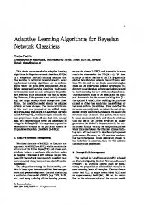
(a) NASA dataset Fig. 1.
(b) PRISM dataset
LANDSAT scenes used in the experiments.
pixels computed in terms of spectral features, Gabor and cooccurrence texture features, and elevation information from Digital Elevation Model (DEM) data. Region level representations include land cover labels for groups of pixels obtained through segmentation. These labels are learned from statistical summaries of pixel contents of regions using mean, standard deviation and histograms, and from shape information like area, boundary roughness, orientation and moments. Scene level representations include interactions of different regions computed in terms of spatial relationships. Visual grammar consists of two learning steps. First, pixel level models are learned using naive Bayes classifiers that provide a probabilistic link between low-level image features and high-level user-defined semantic labels. Then, these pixels are merged using region growing to find region level labels. Second, a Bayesian framework is used to learn scene classes based on automatic selection of distinguishing spatial relationships between regions. Details of these learning algorithms are given in the following sections. Examples in the rest of the paper use LANDSAT scenes of Washington, D.C., obtained from the NASA Goddard Space Flight Center, and Washington State and Southern British Columbia obtained from the PRISM project at the University of Washington. We use spectral values, Gabor texture features [11] and hierarchical segmentation features [12] for the first dataset, and spectral values, Gabor features and DEM data for the second dataset, shown in Fig. 1. III. P ROTOTYPE R EGIONS The first step to construct a visual grammar is to find meaningful and representative regions in an image. Automatic extraction of regions is required to handle large amounts of data. To mimic the identification of regions by experts, we define the concept of prototype regions. A prototype region is a region that has a relatively uniform low-level pixel feature distribution and describes a simple scene or part of a scene.
Ideally, a prototype is frequently found in a specific class of scenes and differentiates this class of scenes from others. In previous work [9], [10], we used automatic image segmentation and unsupervised model-based clustering to automate the process of finding prototypes. In this paper, we extend this prototype framework to learn prototype models using Bayesian classifiers with automatic fusion of features. Bayesian classifiers allow subjective prototype definitions to be described in terms of objective attributes. These attributes can be based on spectral values, texture, shape, etc. Bayesian framework is a probabilistic tool to combine information from multiple sources in terms of conditional and prior probabilities. We can create a probabilistic link between low-level image features and high-level user-defined semantic land cover labels (e.g. city, forest, field). Assume there are k prototype labels defined by the user. Let x1 , . . . , xm be the attributes computed for a pixel. The goal is to find the most probable prototype label for that pixel given a particular set of values of these attributes. The degree of association between the pixel and prototype j can be computed using the posterior probability p(j|x1 , . . . , xm ) p(x1 , . . . , xm |j)p(j) = p(x1 , . . . , xm ) p(x1 , . . . , xm |j)p(j) = p(x1 , . . . , xm |j)p(j) + p(x1 , . . . , xm |¬j)p(¬j) Qm p(j) i=1 p(xi |j) Q Qm = m p(j) i=1 p(xi |j) + p(¬j) i=1 p(xi |¬j)
(1)
under the conditional independence assumption. The parameters for each attribute model p(xi |j) can be estimated separately and this simplifies learning. Therefore, user interaction is only required for the labeling of pixels as positive (j) or negative (¬j) examples for a particular prototype label under training. Then, the predicted prototype becomes the one with the largest posterior probability and the pixel is assigned the prototype label j ∗ = arg max p(j|x1 , . . . , xm ). j=1,...,k
(2)
We use discrete variables in the Bayesian model where continuous features are converted to discrete attribute values using an unsupervised clustering stage based on the k-means algorithm. In the following, we describe learning of the models for p(xi |j) using the positive training examples for the j’th prototype label. Learning of p(xi |¬j) is done the same way using the negative examples. For a particular prototype, let each discrete variable xi have ri possible values (states) with probabilities p(xi = z|θ i ) = θ iz > 0 i {θ i z }rz=1
(3)
is the set of where z ∈ {1, . . . , ri } and θ i = parameters for the i’th attribute model. This corresponds to a multinomial distribution. To be able to do estimation with a very small training set D, we use the conjugate prior, the Dirichlet distribution p(θ i ) = Dir(θ i |αi1 , . . . , αiri ) where αiz
Fig. 2. Training for the city prototype. Positive and negative examples of city pixels in the image on the left are used to learn a Bayesian classifier that creates the probability map shown on the right. Brighter values in the map show pixels with high probability of being part of a city. Pixels marked with red have probabilities above 0.9.
are positive constants. Then, the posterior distribution of θ i can be computed using the Bayes rule as p(D|θ i )p(θ i ) p(D) = Dir(θ i |αi1 + Ni1 , . . . , αiri + Niri )
p(θ i |D) =
(4)
where Niz is the number of cases in D in which xi = z, and the Bayes estimate for θ iz can be found by taking the conditional expected value αiz + Niz θˆiz = Ep(θi |D) [θ iz ] = (5) αi + N i Pr i Pr i where αi = z=1 Niz . An intuitive z=1 αiz and Ni = choice for the hyper-parameters αi1 , . . . , αiri for the Dirichlet prior is to assume all ri states to be equally probable and set αiz = 1, ∀z ∈ {1, . . . , ri } where 1 + Niz θˆi z = . ri + Ni
(6)
Given the current state of the classifier that was trained using the prior information and the sample D, we can easily update the parameters when new data D 0 is available. The new posterior distribution for θ i becomes p(θ i |D, D0 ) =
p(D0 |θ i )p(θ i |D) . p(D0 |D)
(7)
With the Dirichlet priors and the posterior distribution for p(θ i |D) given in (4), the updated posterior distribution becomes 0 0 ) p(θ i |D, D0 ) = Dir(θ i |αi1 +Ni1 +Ni1 , . . . , αiri +Niri +Nir i (8) 0 where Niz is the number of cases in D 0 in which xi = z. Hence, updating the classifier parameters involves only updating the counts in the estimates for θˆiz . Figs. 2 and 3 illustrate learning of prototype models from positive and negative examples.
Fig. 3.
Training for the park prototype.
Given the models learned for all user-defined semantic prototype labels, a new image can be segmented into spatially contiguous regions as follows: • Compute probability maps for all labels and assign each pixel to one of the labels using the maximum a posteriori probability (MAP) rule. There is also a reject class for probabilities smaller than a threshold and these pixels are marked as background. • After each pixel is assigned to a prototype, merge the pixels with identical labels to find regions. Small regions can also be marked as background using connected components analysis. • Finally, use region growing to assign background pixels to the foreground regions by placing a window at each background pixel and assigning it to the label that occurs the most in its neighborhood. The resulting regions are characterized by their polygon boundaries and also propagate the corresponding pixel level labels. Fig. 4 shows example segmentations. Bayesian classifiers successfully learned proper combinations of features for particular prototypes. For example, using only spectral features confused cities with residential areas and some parks with fields. Using the same training examples, adding Gabor features improved some of the models but caused more confusion between parks and fields. Finally adding hierarchical segmentation features [12] fixed most of the confusions and enabled learning of accurate models from a small set of training examples. IV. S PATIAL R ELATIONSHIPS After images are segmented and prototype labels are assigned to all regions, the next step in the construction of the visual grammar is modeling of region spatial relationships. The regions of interest are usually the ones that are close to each other. Representations of spatial relationships depend on the representations of regions. V ISI M INE models regions by their boundary polygons. We use fuzzy modeling of pairwise spatial
Fig. 5. Spatial relationships of region pairs: disjoined, bordering, invaded by, surrounded by, near, far, right, left, above and below.
centroid of the first region, νi centroid of the second region, νj • angle between the horizontal (column) axis and the line joining the centroids, θij where i, j ∈ {1, . . . , n} and n is the number of regions in the image. Then, each region pair can be assigned a degree of their spatial relationship using the fuzzy class membership functions given in Fig. 6. For the perimeter-class relationships, we use the perimeter ratios rij with trapezoid membership functions. The motivation for the choice of these functions is as follows. Two regions are disjoined when they are not touching each other. They are bordering each other when they have a common perimeter. When the common perimeter between two regions gets closer to 50%, the larger region starts invading the smaller one. When the common perimeter goes above 80%, the relationship is considered an almost complete invasion, i.e. surrounding. For the distance-class relationships, we use the perimeter ratios rij and boundary polygon distances dij with sigmoid membership functions. For the orientation-class relationships, we use the angles θij with truncated cosine membership functions. Details of the membership functions are given in [10]. Note that the pairwise relationships are not always symmetric. Furthermore, some relationships are stronger than others. For example, surrounded by is stronger than invaded by, and invaded by is stronger than bordering, e.g. the relationship “small region invaded by large region” is preferred over the relationship “large region bordering small region”. The class membership functions are chosen so that only one of them is the largest for a given set of measurements. When an area of interest consists of multiple regions, this area can be decomposed into multiple region pairs and the measurements defined above can be computed for each of the pairwise relationships. For an area that consists of k regions, •
•
Fig. 4. Segmentation examples from the NASA dataset. Images on the left column are segmented using models for city (red), residential area (cyan), water (blue), park (green), field (yellow) and swamp (maroon). Images on the right column show resulting regions and their prototype labels.
relationships to describe the high-level user concepts shown in Fig. 5. Among these relationships, disjoined, bordering, invaded by and surrounded by are perimeter-class relationships, near and far are distance-class relationships, and right, left, above and below are orientation-class relationships. These relationships are divided into sub-groups because multiple relationships can be used to describe a region pair, e.g. invaded by from left, bordering from above, and near and right, etc. To find the relationship between a pair of regions represented by their boundary polygons, we first compute • • • • •
perimeter of the first region, πi perimeter of the second region, πj common perimeter between two regions, πij ratio of the common perimeter to the perimeter of the π first region, rij = πiji closest distance between the boundary polygon of the first region and the boundary polygon of the second region, dij
1.0
the “min” operator, which is the equivalent of the Boolean ¡ ¢ “and” operator in fuzzy logic, can be used to combine k2 pairwise relationships.
0.6 0.4 0.0
0.2
Fuzzy membership value
0.8
V. I MAGE C LASSIFICATION DISJOINED BORDERING INVADED_BY SURROUNDED_BY
0.0
0.2
0.4
0.6
0.8
1.0
Perimeter ratio
0.4
0.6
FAR NEAR
0.0
0.2
Fuzzy membership value
0.8
1.0
(a) Perimeter-class spatial relationships
0
100
200
300
400
500
600
Distance
0.4
0.6
RIGHT ABOVE LEFT BELOW
0.0
0.2
Fuzzy membership value
0.8
1.0
(b) Distance-class spatial relationships
-4
-3
-2
-1
0
1
2
3
4
Theta
(c) Orientation-class spatial relationships Fig. 6.
Fuzzy membership functions for pairwise spatial relationships.
Image classification is defined here as a problem of assigning images to different classes according to the scenes they contain. The visual grammar enables creation of higher level classes that cannot be modeled by individual pixels or regions. Furthermore, learning of these classifiers require only a few training images. We use a Bayesian framework that learns scene classes based on automatic selection of distinguishing (e.g. frequently occurring, rarely occurring) relations between regions. The input to the system is a set of training images that contain example scenes for each class defined by the user. Let s be the number of classes, m be the number of relationships defined for region pairs, k be the number of regions in a region group, and t be a threshold for the number of region groups that will be used in the classifier. Denote the classes by w1 , . . . , ws . The system automatically learns classifiers from the training data as follows: 1) Count the number of times each possible region group with a particular spatial relationship is found in the set of training images for each class. This is a combinatorial problem because the total number of region groups in ¡ ¢ an image with n regions is nk and the total number of ¡m+(k2)−1¢ possible relationships in a region group is . (k2) A region group of interest is the one that is frequently found in a particular class of scenes but rarely exists in other classes. For each region group, this can be measured using class separability which can be computed in terms of within-class and between-class variances of the counts as ¶ µ 2 σB (9) ς = log 1 + 2 σW Ps 2 where σW = i=1 vi var{zj | j ∈ wi } is the withinclass variance, vi is the number of training images for class wi , zj is the number of times thisPregion group 2 = var{ j∈wi zj | i = is found in training image j, σB 1, . . . , s} is the between-class variance, and var{·} denotes the variance of a sample. 2) Select the top t region groups with the largest class separability values. Let x1 , . . . , xt be Bernoulli random variables for these region groups, where xj = T if the region group xj is found in an image and xj = F otherwise. Let p(xj = T ) = θj . Then, the number of times xj is found ¡ in¢ vimages from class wi has a Binomial(vi , θj ) = vviji θj ij (1 − θj )vi −vij distribution where vij is the number of training images for wi that contain xj . Using a Beta(1, 1) distribution as the conjugate prior, the Bayes estimate for θj becomes p(xj = T |wi ) =
vij + 1 . vi + 2
(10)
Using a similar procedure with Multinomial and Dirichlet distributions, the Bayes estimate for an image belonging to class wi (i.e. containing the scene defined by class wi ) is computed as vi + 1 p(wi ) = Ps . i=1 vi + s
(11)
3) For an unknown image, search for each of the t region groups (determine whether xj = T or xj = F, ∀j) and assign that image to the best matching class using the MAP rule with the conditional independence assumption as
(a) Training images
w∗ = arg max p(wi |x1 , . . . , xt ) wi
= arg max p(wi ) wi
t Y
p(xj |wi ).
(12)
j=1
Classification examples from the PRISM dataset are given in Figs. 7–9. We used four training images for each of the classes defined as “clouds”, “residential areas with a coastline”, “tree covered islands”, “snow covered mountains”, “fields” and “high-altitude forests”. Commonly used statistical classifiers require a lot of training data to effectively compute the spectral and textural signatures for pixels and also cannot do classification based on high-level user concepts because of the lack of spatial information. Rule-based classifiers also require significant amount of user involvement every time a new class is introduced to the system. The classes listed above provide a challenge where a mixture of spectral, textural, elevation and spatial information is required for correct identification of the scenes. For example, pixel level classifiers often misclassify clouds as snow and shadows as water. On the other hand, the Bayesian classifier described above can successfully eliminate most of the false alarms by first recognizing regions that belong to cloud and shadow prototypes and then verify these region groups according to the fact that clouds are often accompanied by their shadows in a LANDSAT scene. Other scene classes like residential areas with a coastline or tree covered islands cannot be identified by pixel level or scene level algorithms that do not use spatial information. The visual grammar classifiers automatically learned the distinguishing region groups that were frequently found in particular classes of scenes but rarely existed in other classes.
(b) Images classified as containing clouds Fig. 7. Classification results for the “clouds” class which is automatically modeled by the distinguishing relationships of white regions (clouds) with their neighboring dark regions (shadows).
(a) Training images
VI. C ONCLUSIONS We described a visual grammar that aims to bridge the gap between low-level features and high-level semantic interpretation of images. The system uses naive Bayes classifiers to learn models for region segmentation and classification from automatic fusion of features, fuzzy modeling of region spatial relationships to describe high-level user concepts, and Bayesian classifiers to learn image classes based on automatic selection of distinguishing (e.g. frequently occurring, rarely occurring) relations between regions. The visual grammar overcomes the limitations of traditional region or scene level image analysis algorithms which assume
(b) Images classified as containing tree covered islands Fig. 8. Classification results for the “tree covered islands” class which is automatically modeled by the distinguishing relationships of green regions (lands covered with conifer and deciduous trees) surrounded by blue regions (water).
negative examples for the classes defined by the user. We demonstrated our system with classification scenarios that could not be handled by traditional pixel, region or scene level approaches but where the visual grammar provided accurate and effective models. R EFERENCES (a) Training images
(b) Images classified as containing residential areas with a coastline Fig. 9. Classification results for the “residential areas with a coastline” class which is automatically modeled by the distinguishing relationships of regions containing a mixture of concrete, grass, trees and soil (residential areas) with their neighboring blue regions (water).
that the regions or scenes consist of uniform pixel feature distributions. Furthermore, it can distinguish different interpretations of two scenes with similar regions when the regions have different spatial arrangements. The system requires only a small amount of training data expressed as positive and
[1] S. I. Hay, M. F. Myers, N. Maynard, and D. J. Rogers, Eds., Photogrammetric Engineering & Remote Sensing, vol. 68, no. 2, February 2002. [2] K. Koperski, G. Marchisio, S. Aksoy, and C. Tusk, “VisiMine: Interactive mining in image databases,” in Proceedings of IEEE International Geoscience and Remote Sensing Symposium, vol. 3, Toronto, Canada, June 2002, pp. 1810–1812. [3] J. R. Smith and S.-F. Chang, “VisualSEEk: A fully automated contentbased image query system,” in Proceedings of ACM International Conference on Multimedia, Boston, MA, November 1996, pp. 87–98. [4] S. Berretti, A. D. Bimbo, and E. Vicario, “Modelling spatial relationships between colour clusters,” Pattern Analysis & Applications, vol. 4, no. 2/3, pp. 83–92, 2001. [5] P. J. Neal, L. G. Shapiro, and C. Rosse, “The digital anatomist structural abstraction: A scheme for the spatial description of anatomical entities,” in Proceedings of American Medical Informatics Association Annual Symposium, Lake Buena Vista, FL, November 1998. [6] W. W. Chu, C.-C. Hsu, A. F. Cardenas, and R. K. Taira, “Knowledgebased image retrieval with spatial and temporal constructs,” IEEE Transactions on Knowledge and Data Engineering, vol. 10, no. 6, pp. 872–888, November/December 1998. [7] L. H. Tang, R. Hanka, H. H. S. Ip, and R. Lam, “Extraction of semantic features of histological images for content-based retrieval of images,” in Proceedings of SPIE Medical Imaging, vol. 3662, San Diego, CA, February 1999, pp. 360–368. [8] E. G. M. Petrakis and C. Faloutsos, “Similarity searching in medical image databases,” IEEE Transactions on Knowledge and Data Engineering, vol. 9, no. 3, pp. 435–447, May/June 1997. [9] S. Aksoy, G. Marchisio, K. Koperski, and C. Tusk, “Probabilistic retrieval with a visual grammar,” in Proceedings of IEEE International Geoscience and Remote Sensing Symposium, vol. 2, Toronto, Canada, June 2002, pp. 1041–1043. [10] S. Aksoy, C. Tusk, K. Koperski, and G. Marchisio, “Scene modeling and image mining with a visual grammar,” in Frontiers of Remote Sensing Information Processing, C. H. Chen, Ed. World Scientific, 2003, pp. 35–62. [11] G. M. Haley and B. S. Manjunath, “Rotation-invariant texture classification using a complete space-frequency model,” IEEE Transactions on Image Processing, vol. 8, no. 2, pp. 255–269, February 1999. [12] J. C. Tilton, G. Marchisio, and M. Datcu, “Image information mining utilizing hierarchical segmentation,” in Proceedings of IEEE International Geoscience and Remote Sensing Symposium, vol. 2, Toronto, Canada, June 2002, pp. 1029–1031.