Learning Causal Rules Kamran Karimi and Howard J. Hamilton Technical Report CS-2001-03 December, 2001
Copyright © 2001 Kamran Karimi and Howard J. Hamilton Department of Computer Science University of Regina Regina, Saskatchewan CANDA S4S 0A2
ISSN 0828-3494 ISBN 0-7731-0430-5
Learning Causal Rules Kamran Karimi and Howard J. Hamilton Department of Computer Science University of Regina Regina, Saskatchewan Canada S4S 0A2 {karimi, hamilton}@cs.uregina.ca This technical report is available online at http://www.cs.uregina.ca/~karimi/learning.html
Table of Contents 1. Introduction 2. Problem Description 3. Standard Problems 4. Publications 5. Software 6. Other Tools and Approaches 7. Contact Us! 8. Bibliography
1.
Introduction
Finding the cause of things has always been a main focus of human curiosity. As part of a project at the Department of Computer Science at the University of Regina, we are using existing tools to extract causal (temporal) and association (non-temporal) rules from observational data. We have successfully used C4.5 to extract such rules. By a causal rule, we mean a rule that involves variables that are observed at different time. In an association rule, on the other hand, all the variables are seen at the same time, so there is little doubt that no causal relation exists. The main emphasis is on making the process of discovering causal rules automatic. This requires relying as little as possible for a human being to provide information about the domain where the variables are observed. This project has had a number of byproducts which can be useful independent of the original goals of the project. For example, C4.5 has been modified to output the rules it discovers in PROLOG. We have also changed C4.5 to respect any temporal order that may exist in the data. Some of the software we have developed can be downloaded from the Software section of this document. The published papers describing our work can be found at the Publications section.
2. Problem Description We consider the problem of discovering relations among a set of variables that represent the state of a single system as time progresses. Values of the variables are recorded at different times, giving a sequence of temporally ordered records without a distinguished time variable. This data will then be used to discover rules that apply to the system under investigation. Our aim is to identify as many cases as possible where two or more variables' values depend on each other. Knowing this would allow us to explain how the system may be working. We may also want to control some of the variables by changing the values of other variables. For example, if we observe that (y = 5) is always
1
true when (x = 2), then we could predict the value of y as 5 when we see that x is 2. This is an example of association between two values, where observing the value of one variable allows us to predict the value another variable, without one necessarily causing the other. Alternatively, we could assume that we have the rule: if {(x = 5)} then (y = 2), and use it to set the value of y to 2 by setting the value of x to 5. This rule can be interpreted as a causal relation or an association. The exact nature of the rules is very hard to determine from the inside of the domain. Any decision to interpret such rules as indicating causal relations requires knowledge from outside the domain under investigation. The learning takes place in two phases. In phase one, the aim is to gather information about the response of the environment to the actions we are interested in. We consider the experimenter and the environment to form one system. Experiments are conducted, in which certain variables of the system are recorded. In phase 2, these observations are used to learn relationships about the variables of the system. The relationships constitute our output. In Figure 1 we see a robot in a very simple world. The robot can move Up, Down, Left or Right. There may be obstacles and sources of energy in the world.
Figure 1. The Robot can move in four directions
In Figure 2 we see two sample walks. One starts from the creature's current position. It gets to the vicinity of an obstacle, fails to enter into position of the obstacle, and continues up. In the second walk, the creature reaches the power source.
2
Figure 2. A robot moving around
3. Standard Problems We present a few problems that can be approached with our method. They are all conceptually simple. The common thing among them is a stable environment, where the rules that govern do not change as time passes.
Learning the rules in the URAL (University of Regina Artificial Life) Simulator URAL is a discrete event simulator with well known rules that govern the artificial environment. There is little ambiguity about what causes what. This helps to judge the quality of the discovered rules. The world in URAL is made of a two dimensional board with one or more agents (called creatures in Artificial Life literature) living in it. An agent moves around and if it finds food, eats it. Food is produced by the simulator and placed at positions that are randomly determined at the start of each run of the simulator. There is a maximum for the number of positions that may have food at any one time, so a position that was determined as capable of having food may or may not have food at a given time. The agent can sense its position and also the presence of food at its current position. At each time-step, it randomly chooses to move from its current position to Up, Down, Left, or Right. It cannot get out of the board, or go through the obstacles that are placed in the board by the simulator. In such cases, a move action will not change the agent's position. The agent can sense which action it takes in each situation. The aim is to learn the effects of its actions at each particular place. Figure 3 shows a simulated world with some obstacles and food at different positions.
3
Figure 3. An example URAL world In figure 4 we see a sample sequence of the agent's observations. It consists of its present x and y values, whether or not food is present at that location, and the action that the agent performs at that time step. The results of the action will be known in the next time step. Figure 4. Observations of a creature Figure 5 shows the records after they have been flattened, that is, combined with the preceding and the succeeding records, to bring the causes (actions) and the effects (next position) together in the same record. The number of records involved in the flattening process is determined by the time window. In Figure 5 we have used a time window of 2, because the results of actions will be known in the next time step. Time is relative, and supposed to begin at the start of each flattened record. x1, y1, Food1 and Action1 thus belong to the previous time step, while x2, y2, Food2 and Action2 belong to the next time step. Figure 5. Flattened data Moving vertically and horizontally are independent of each other in this world, So in the absence of any obstacles on the world we could have rules like: General rule for moving Right. No obstacles on the board if (x1 = a AND Action1 = Right) then if(a < World_Width) then
4
x2 = a + 1 else x2 = a General rule for moving Left. No obstacles on the board if (x1 = a AND Action1 = Left) then if(a > 0) then x2 = a - 1 else x2 = a General rule for moving Down. No obstacles on the board if (y1 = a AND Action1 = Down) then if(a < World_Height) then y2 = a + 1 else y2 = a General rule for moving Up. No obstacles on the board if (y1 = a AND Action1 = Up) then if(a > 0) then y2 = a - 1 else y2 = a These 4 rules are all that are needed to specify the effects of the agent's movements. If there are obstacles on the board, the rules will be more complex, because the result of a move action depends of whether there is an obstacle in the vicinity. In this case the location of the obstacle should be reflected in the rule. The rules for moving when there is a single obstacle at (3, 5) that would fail the rule is: Moving Right in the presence of an obstacle if(x1 = 2 AND y1 = 5 AND Action1 = Right) then x2 = 2 Moving Left in the presence of an obstacle if(x1 = 4 AND y1 = 5 AND Action1 = Left) then x2 = 4 Moving Down in the presence of an obstacle if(x1 = 3 AND y1 = 4 AND Action1 = Down) then y1 = 4 Moving Up in the presence of an obstacle if(x1 = 3 AND y1 = 6 AND Action1 = Up) then y2 = 6 The general rules apply in all other location on the board. Obstacles create exceptions to the general rules that exist in a world without them, and there is no way to get around them. The best way to represent a world that contains obstacles is to enumerate all the exceptions first, and then give the general rule as a "catch-all" or default behaviour. The actual output extracted from URAL's data depends on the application used. For example, C4.5 can not output general rules. Any rule output by C4.5 will use explicit values for the variables. The following example rules show this more clearly:
5
C4.5 rule to handle moving to the right in the absence of any obstacles on the board if(x1 = 1 AND Action1 = Right) Then x2 = 2 if(x1 = 2 AND Action1 = Right) Then x2 = 3 ... What happens at the edge of the world is shown in by the next rule: C4.5 rule to handle the moving beyond the edge in a 10 by 10 world if(x1 = 10 AND Action1 = Right) then x2 = 10 We see that C4.5 can prune other variables like y1, y2, food1, food2 and Action2 from the rules.
Industrial Robot. An industrial robotic arm has certain abilities. It can move itself in different directions, and its sensors allow it to know its own position after a move. The aim is to place the top of the arm in a desired grid. Going from one position to another often requires a series of movements that gradually changes the robotic arm so it reaches the desired position. The problem is to make the robot able to do its own planning. The robot can thus be introduced to a new place, allowed to run experiments, and then learn the rules. This reduces the need for programming the robot for every new situation. Figure 6 shows two different configurations for a robotic arm, such as a welder, with 2 degrees of freedom. Each joint can move to the left or right (2D movements). The first joint which holds the first stub can be anywhere from 10 degrees to 170 degrees relative to the horizontal plane, while the second stub, moved by the second joint, can be at 10 degrees to 350 degrees relative to the first stub. A device at the end of the second stub can detect its position, and determine its current grid location. At left, we see the initial configuration, and at right a desired configuration is shown. If the robot has been in both positions (maybe while randomly moving around, or maybe because an "instructor" moved it step by step), then it would be desirable for the robot to send the appropriate commands to its joints by itself the next time it needs to go from one grid to the next.
Figure 6. A robotic arm at different grid locations The joints can either Hold their current positions, or either increase their angle or decrease it. Sample data generated by such an arm could like Figure 7. We assume that the sensors is originally positioned in position (1,1), and see how it goes to position (1,2).
6
Figure 7. Observed values, saved in records If the exact location of the sensor can not be determined because it is in the middle of two positions (here: (1,1) and (1,2)), then the current configuration of the system is used instead. This is achieved by pasting the position of the two joints together. We use a distinct variable for the Position (instead of simply using the two Joint variables) because we want to be able to differentiate between positions of interest like (1,1) and (1,2) vs. other "intermediate" positions. To extract rules for the arm's movement we flatten them based on the position. The data in Figure 7 can be flattened as shown in Figure 8 below. Figure 8. Flattened data The ideal set of rules for this environment would take a starting position, a destination, and then output a series of commands to the joints that have to be followed in order to get to the destination. An "step-by-step rule" does not specify a sequence of actions that have to be performed over time, but only the actions that should be performed at a single time step. The rules extracted by C4.5 from URAL's data are an example of such rules. Having rules that determine the movement of the robot step by step means that there will be many rules to handle. One advantage of having step by step rules is that they allow for some fault tolerance. Each rule examines the current situation and then outputs an action that should be performed to go to another situation. If for any reason the action fails, and the desired situation can not be reached, then the actual situation can be used to find another rule to fire. We would be interested in rules that look like this: if(current_p = 11 AND Action1 = Hold AND Action2 = Inc) then Next_p = 0516 ... if(current_p = 0717 AND Action1 = Hold AND Action2 = Inc) then Next_p = 12 We can use the current position of the joints to go to any desired location by following a chain of such rules.
7
The Wumpus Game Wumpus is a game of strategy and luck. Implementations of this game for many computer platforms are available. The setup is like that of URAL: In a dark dungeon, an agent (human or otherwise) wanders from room to room, trying to find gold, while avoiding the feared Wumpus. The agent can use signs to know what is to be found in a neighboring room. This gives the Wumpus agent more information than the agent in URAL, because the Wumpus agent can know about its neighboring locations as well as the current one. For example, stench would indicate that the Wumpus is in the room or one of its neighbors. In the same manner a breeze indicates a pit, falling into which would be fatal. The agent should use these signs to find the gold and get out of the dungeon safely. Figure 9 shows an example Wumpus world.
Figure 9. An example Wumpus World Sample data gathered by the agent in the Wumpus world could look as shown in Figure 10. Notice that We assume the agent never gets really destroyed. Figure 10. Data gathered from a Wumpus world The desired rules in this domain are more varied in nature. For example, while the rules concerning the pits (breeze) and the gold depend of location (so that the x and y location can be substituted for the presence of breeze, for example), the rule about the Wumpus creature does not apply always in the same location because as the creature
8
moves, the stink moves with it. Another difficulty in the Wumpus world is that the sensation of feeling the breeze or the stink does not give definite information about where the source is. For a human player who will lose the game if he encounters the Wumpus or falls into a pit, the safest move upon feeling a stink or breeze is to move back to the previous position, since any other move could be fatal. Humans can extract this simple rule by using their analyzing abilities and imagining what would happen if they did actually move to a different location. The assumption that he agent will not be destroyed helps it in discovering the location of the gold and the pits, but the location of the Wumpus creature can never be determined definitely by any rule unless we assume that the creature is stationary. This example differs from the previous ones because the causal rules are not the same for the designer and the agent living in the world. From the designer's perspective, the rules for stink are these: If(wumpus_at(x, y)) then { if(x < world_Width) then stink_at(x+1, y) if(x > 0) then stink_at(x-1, y) if(y < World_length) then stink_at(x, y+1) if(y > 0) then stink_at(x, y-1) } This rule implies that the presence of stink is caused by the presence of the wumpus because the existence of the wumpus precedes the stink. However, the agent does not experience the world like this. For the agent, the stink is felt first, and then the wumpus is encountered, so the temporal order is reversed. As far as the agent is concerned, the stink "causes" the wumpus. So the agent will find rules that look like this: if(stink_at(x,y)) then wumpus_at(x+1, y) OR wumpus_at(x-1, y) OR wumpus_at(x, y+1) OR wumpus_at(x, y-1) The same type of rules could be discovered for the presence of the pit. However, For the pit locations, the rules can be considerably simpler because the agent can discover the exact location of the pit. So assuming that a pit exists at location (3,4), the corresponding rule would be: pit_at(3,4) This confirms the notion that causality is a subjective experience. Determining a causal relation with absolute certainty requires knowing the system under investigation very well. This puts limits on the causal rules that can be determined by any method. The agent is merely observing the environment. Neither the sensation (smell or breeze) nor the "cause" (from the designer's point of view: presence of Wumpus or a pit) are under the agent's control. As a result, the method of changing one variable and measuring the change in others does not work. Many tools currently used to discover causal relations look for variables that change together to discover causal relationship among them. Covariance is a popular measure in this method. One problem with this method is that most these tools do not consider a time to have been past between the observation of the variables. This makes it hard to define a direction for the causal relationship (which variable changes first, and which one changes later).
??? Let us know about other problems!
9
4. Publications The following papers are available from http://www.cs.uregina.ca/~karimi/pubs.html •
Kamran Karimi and Howard J. Hamilton, Finding Temporal Relations: Causal Bayesian Networks vs. C4.5, The Twelfth International Symposium on Methodologies for Intelligent System (ISMIS'2000), Charlotte, NC, USA, October 2000. This paper appears in the LNCS Series, © Springer-Verlag. (Also available in HTML format) .
•
Kamran Karimi and Howard J. Hamilton, Learning With C4.5 in a Situation Calculus Domain,The Twentieth SGES International Conference on Knowledge Based Systems and Applied Artificial Intelligence (ES2000), Cambridge, UK, December 2000. This paper is published by Springer-Verlag London. (Also available in HTML format).
•
Kamran Karimi and Howard J. Hamilton, Logical Decision Rules: Teaching C4.5 to Speak Prolog, The Second International Conference on Intelligent Data Engineering and Automated Learning (IDEAL 2000), Hong Kong, December 2000. This paper appears in the LNCS Series, © Springer-Verlag. (Also available in HTML format)
5.
Software
The following software/patches are available for download from http://www.cs.uregina.ca/~karimi/downloads.html •
URAL is an artificial life simulator written in Java.
•
A patch file to make C4.5 Release 8 output PROLOG statements
•
A patch file to make C4.5 Release 8 respect temporal order in its output
•
RFCT is an unsupervised extension of C4.5 that allows the discovery of temporal and causal rules. RFCT is written in Java and includes a graphical user interface.
6. •
Other Tools and Approaches Casual Bayesian Networks are a popular method of discovering causal relationships among variables. TETRAD and Webweaver are two such programs. TETRAD is a famous tool for extracting causal relationships from statistical data. WebWeaver constructs Bayesian networks that can be used for inference purposes.
•
Situation Calculus has been used widely to specify the effects of actions. In most cases, these causal rules must be written down by a domain expert. GOLOG is a programming language that allows domain experts to write situation calculus statements.
•
??? Let us know about other tools and approaches!
10
7.
Contact Us!
We would be happy to know your opinion about this work. Please contact us if you know of other applications where the approach presented in this page could be useful. We would also like to add links to sites with other approaches to learning causal rules, and any help is appreciated. You can email us at: Howard J. Hamilton:
[email protected] Kamran Karimi:
[email protected] Our Address is: Department of Computer Science University of Regina Regina, Saskatchewan Canada S4S 0A2 fax: (+1 306) 585 4745
8.
Bibliography
[1] Agrawal R. and Srikant R., Mining Sequential Patterns, Proceedings of the International Conference on Data Engineering (ICDE), Taipei, Taiwan, March 1995. [2] Blake, C.L and Merz, C.J., UCI Repository of machine learning databases, Irvine, CA: University of California, Department of Information and Computer Science, 1998. [3] Bowes, J., Neufeld, E., Greer, J. E. and Cooke, J., A Comparison of Association Rule Discovery and Bayesian Network Causal Inference Algorithms to Discover Relationships in Discrete Data, Proceedings of the Thirteenth Canadian Artificial Intelligence Conference (AI'2000), Montreal, Canada, 2000. [4] Berndt, D.J. and Clifford, J., Finding Patterns in Time Series: A Dynamic Programming Approach, Advances in Knowledge Discovery and Data Mining, U.M. Fayyad, G. Piatetsky-Shapiro, P. Smyth, et al. (eds.), AAAI Press/ MIT Press, pp. 229-248, 1996. [5] Clocksin, W.F., Melish, C.S, Programming in Prolog, Springer Verlag, 1984. [6] Freedman, D. and Humphreys, P., Are There Algorithms that Discover Causal Structure?, Technical Report 514, Department of Statistics, University of California at Berkeley, 1998. [7] Guralnik, V., Wijesekera, D. and Srivastava, J., Pattern Directed Mining of Sequence Data, Proceedings of the Fourth International Conference on Knowledge Discovery & Data Mining (KDD-98), 1998. [8] Heckerman, D., A Bayesian Approach to Learning Causal Networks, Microsoft Technical Report MSR-TR-9504, Microsoft Corporation, May 1995. [9] Humphreys, P. and Freedman, D., The Grand Leap, British Journal of the Philosophy of Science 47, pp. 113123, 1996. [12] Korb, K. B. and Wallace, C. S., In Search of Philosopher's Stone: Remarks on Humphreys and Freedman's Critique of Causal Discovery, British Journal of the Philosophy of Science 48, pp. 543- 553, 1997. [13] Koza, J. R. and Rice, J. P. (1992). Automatic Programming of Robots using Genetic Programming, The Tenth National Conference on Artificial Intelligence, Menlo Park, CA, USA.
11
[14] Levesque, H. J., Reiter, R., Lesp‚rance, Y., Lin, F. and Scherl. R. (1997). GOLOG: A Logic Programming Language for Dynamic Domains, Journal of Logic Programming, No. 31, pp. 59-84. [15] Levy, S., Artificial Life: A Quest for a New Creation, Pantheon Books, 1992. [16] Lin F. and Reiter, R. (1997). Rules as actions: A Situation Calculus Semantics for Logic Programs, Journal of Logic Programming Special Issue on Reasoning about Action and Change, 31(1-3), pp.299-330. [17] Mannila, H., Toivonen, H. and Verkamo, A. I., , Discovering Frequent Episodes in Sequences, Proceedings of the First International Conference on Knowledge Discovery and Data Mining, pp. 210-215, 1995. [18] McCarthy, J. and Hayes, P. C. Some Philosophical Problems from the Standpoint of Artificial Intelligence, Machine Intelligence 4, 1969. [19] Moore, R. C., The Role of Logic in Knowledge Representation and Commonsense Reasoning. Readings in Knowledge Representation, Morgan Kaufmann, pp. 335-341, 1985. [20] Nadel, B. A., Constraint Satisfaction Algorithms, Computational Intelligence, No. 5, 1989. [21] Oates, T. and Cohen, P. R., Searching for Structure in Multiple Streams of Data, Proceedings of the Thirteenth International Conference on Machine Learning, pp. 346 - 354, 1996. [22] Poole, D. (1998). Decision Theory, the Situation Calculus, and Conditional Plans,, Link"ping Electronic Articles in Computer and Information Science, Vol. 3, 1988. [23] Quinlan, J. R., C4.5: Programs for Machine Learning, Morgan Kaufmann, 1993. [24] Roddick, J.F. and Spiliopoulou, M., Temporal Data Mining: Survey and Issues, Research Report ACRC-99007. School of Computer and Information Science, University of South Australia, 1999. [25] Scheines R., Spirtes P., Glymour C. and Meek C., Tetrad II: Tools for Causal Modeling, Lawrence Erlbaum Associates, Hillsdale, NJ, 1994. [26] Silverstein, C., Brin, S., Motwani, R. and Ullman J., Scalable Techniques for Mining Causal Structures, Proceedings of the 24th VLDB Conference, pp. 594-605, New York, USA, 1998. [27] Spirtes, P. and Scheines, R., Reply to Freedman, V. McKim and S. Turner (editors), Causality in Crisis, University of Notre Dame Press, pp. 163-176, 1997. [28] Guralnik, V., Srivastava, J. and Karypis, G., Temporal Decision Tree, Workshop on Mining Scientific Datasets, Minneapolis, June 2000. [29] Console, L., Picardia, C. and Dupre, D. T., Generating Temporal Decision Trees for Diagnosing Dynamic Systems, Eleventh International Workshop on Principles of Diagnosis (DX-00), Morelia, Michoacen, Mexico, June 2000. [30] Brin, S., Motwani, R., Tsur, D. and Ullman, J., Dynamic Itemset Counting and Implication Rules for Market Basket Data, Proceedings of 1997 ACM SIGMOD, Montreal, Canada, June 1997. [31] Chatfield, C., The Analysis of Time Series: An Introduction, Chapman and Hall, 1989. ??? Let us know about other papers and books!
12