appropriate topology, are well suited to represent long term probabilistic de- ...... Giles, C., Hanton, S., and Cowan, J., editors, Advances in Neural Infor-.
Learning Hidden Markov Models to Fit Long-Term Dependencies J. Callut and P. Dupont
Research Report RR 2005-09 July 2005
Abstract We propose in this report a novel approach to the induction of the structure of Hidden Markov Models (HMMs). The notion of partially observable Markov models (POMMs) is introduced. POMMs form a particular case of HMMs where any state emits a single letter with probability one, but several states can emit the same letter. It is shown that any HMM can be represented by an equivalent POMM. The proposed induction algorithm aims at finding a POMM fitting the dynamics of the target machine, that is to best approximate the stationary distribution and the mean first passage times observed in the sample. The induction relies on non-linear optimization and iterative state splitting from an initial order one Markov chain. Experimental results illustrate the advantages of the proposed approach as compared to Baum-Welch HMM estimation or back-off smoothed Ngrams equivalent to variable order Markov chains.
Facult´e des sciences appliqu´ees
UCL Universit´e catholique de Louvain
Learning Hidden Markov Models to Fit Long-Term Dependencies J´erˆome Callut and Pierre Dupont Department of Computing Science and Engineering, INGI Universit´e catholique de Louvain, Place Sainte-Barbe 2, B-1348 Louvain-la-Neuve, Belgium Email: {jcal,pdupont}@info.ucl.ac.be
July 2005 Abstract We propose in this paper a novel approach to the induction of the structure of Hidden Markov Models (HMMs). The notion of partially observable Markov models (POMMs) is introduced. POMMs form a particular case of HMMs where any state emits a single letter with probability one, but several states can emit the same letter. It is shown that any HMM can be represented by an equivalent POMM. The proposed induction algorithm aims at finding a POMM fitting the dynamics of the target machine, that is to best approximate the stationary distribution and the mean first passage times observed in the sample. The induction relies on non-linear optimization and iterative state splitting from an initial order one Markov chain. Experimental results illustrate the advantages of the proposed approach as compared to Baum-Welch HMM estimation or back-off smoothed Ngrams equivalent to variable order Markov chains.
Keywords: HMM topology induction, Partially observable Markov models, Mean first passage times, Lumped Markov process, State splitting algorithm.
Learning Hidden Markov Models to Fit Long-Term Dependencies
1
1
Introduction
Hidden Markov Models (HMMs) are widely used in many pattern recognition areas, including biological sequence modeling [Durbin et al., 1998], speech recognition [Rabiner and Juang, 1993], optical character recognition [Levin and Pieraccini, 1993] and information extraction [Freitag and McCallum, 1999], [Freitag and McCallum, 2000], to name a few. In most cases, the model structure, also referred to as topology, is defined according to some prior knowledge of the application domain. Automatic techniques for inducing the HMM topology are interesting as the structures are sometimes hard to define a priori or need to be tuned after some task adaptation. The work described here presents a new approach towards this objective. Probabilistic automata (PA) form an alternative representation class to model distributions over strings, for which several induction algorithms have been proposed. PA and HMMs actually form two families of equivalent models, according to whether or not final (or termination) probabilities are included. In the former case, the models generate distributions over words of finite length, while, in the later case, distributions are defined over complete finite prefix-free sets [Dupont et al., 2005]. The equivalences between PA and HMMs can be used to apply induction algorithms in either formalism to model the same classes of string distributions. Nevertheless, previous works with HMMs mainly focused either on hand-built models (e.g. [Freitag and McCallum, 1999]) or heuristics to refine predefined structures [Freitag and McCallum, 2000]. More principled approaches are the Bayesian merging technique due to Stolcke [Stolcke, 1994] and the maximum likelihood state-splitting method of Ostendorf and Singer [Ostendorf and Singer, 1997]. The former approach however has not been shown to clearly outperform alternative approaches while the latter is specific to the subclass of left-to-right HMMs modeling speech signals. In contrast, PA induction techniques are often formulated in theoretical learning frameworks. These frameworks typically include adapted versions of the PAC model [Ron et al., 1994], Identification with probability 1 [Carrasco and Oncina, 1999, Denis and Esposito, 2004] or Bayesian learning [Thollard et al., 2000]. Other approaches use error-correcting techniques [Rulot and Vidal, 1988] or statistical tests as a model fit induction bias [Kermorvant and Dupont, 2002]. All the above approaches, while being interesting, are still somehow limited. From the theoretical viewpoint, PAC learnability is only feasible for restricted subclasses of PAs (see [Dupont et al., 2005], for a review). The general PA class is identifiable with probability one [Denis and Esposito, 2004] but this learning framework is weaker than the PAC model. In particular, it
2
INGI Research Report No. 2005-09
guarantees asymptotic convergence to a target model but does not bound the overall computational complexity of the learning process. From a practical viewpoint, several induction algorithms have been applied, typically to some language modeling tasks [Dupont and Chase, 1998, Thollard et al., 2000] [Dupont and Amengual, 2000, Llorens et al., 2002]. Experimental results in these works show that automatically induced PA hardly outperform well smoothed discrete Markov chains (MC), also known as N-grams in this context. Hence even though HMMs and PA are more powerful than simple Markov chains, it is still unclear whether these models should be considered when no strong prior knowledge can help to define their structure. The present contribution describes a novel approach to the structural induction of HMMs. The general objective is to induce the structure and to estimate the parameters of a HMM from a sample assumed to have been drawn from an unknown target HMM. The goal however is not the identification of the target model but the induction of a model sharing with the target the main features of the distribution it generates. We restrict here our attention to features that can be deduced from the sample. These features are closely related to fundamental quantities of a Markov process, namely the stationary distribution and mean first passage times (MFPT). In other words, the induced model is built to fit the dynamics of the target machine observed in the sample, not necessarily to match its structure. We show in section 2 that any HMM can be converted into an equivalent Partially Observable Markov Model (POMM) [Callut and Dupont, 2004]. Any state of a POMM emits a single letter with probability 1, but several states can emit the same letter. Several properties of standard Markov chains are reviewed in section 3. The relation between a POMM and a lumped process in a Markov chain is detailed in section 4. This relation forms the first basis of the induction algorithm presented in section 6. HMMs are able to model a broader class of distributions than finite order Markov chains. In particular, section 5 describes why HMMs, with an appropriate topology, are well suited to represent long term probabilistic dependencies in a compact way. We also argue why accurate modeling of these dependencies cannot be achieved through the classical approach of BaumWelch estimation of a fully connected model. These observations motivate the use of MFPT to guide the search of an appropriate model. The resulting induction algorithm is presented in section 6. Comparative results given in section 7 illustrate the superiority of POMM induction over variable order Markov chains (equivalent to back-off smoothed Ngrams) and EM estimation of a fully connected HMM.
Learning Hidden Markov Models to Fit Long-Term Dependencies 0.4 0.1
3
0.6 1
[a 0.2] [b 0.8]
0.9
0.7
2
0.3
[a 0.9] [b 0.1]
Figure 1: A HMM example.
2
Hidden Markov Models and Partially Observable Markov Models
We recall in this section the classical definition of a HMM and we show that any HMM can be represented by an equivalent partially observable model. Definition 1 (HMM) A discrete Hidden Markov Model (HMM) (with state emission) is a 5-tuple M = hΣ, Q, A, B, ιi where Σ is an alphabet, Q is a set of states, A : Q × Q → [0, 1] is a mapping defining the probability of each transition, B : Q × Σ → [0, 1] is a mapping defining the emission probability of each letter on each state, and ι : Q → [0, 1] is a mapping defining the initial probability of each state. The following stochasticity P (or properness) constraintsPmust be satisfied: ∀q ∈ Q, q0 ∈Q A(q, q 0 ) = 1; P ∀q ∈ Q, a∈Σ B(q, a) = 1; q∈Q ι(q) = 1. Figure 1 presents a HMM defined as follows: Σ = {a, b}, Q = {1, 2}, ι(1) = 0.4; ι(2) = 0.6; A(1, 1) = 0.1; A(1, 2) = 0.9; A(2, 1) = 0.7; A(2, 2) = 0.3; B(1, a) = 0.2; B(1, b) = 0.8; B(2, a) = 0.9; B(2, b) = 0.1 Definition 2 (HMM path) Let M = hΣ, Q, A, B, ιi be a HMM. A path in M is a word defined on Q∗ . For any path ν, νi denotes the i-th state of ν, and |ν| denotes the path length. For any word u ∈ Σ∗ and any path ν ∈ Q∗ , the probabilities PM (u, ν) and PM (u) are defined as follows: Ql−1 ι(ν1 ) i=1 [B(νi , ui )A(νi , νi+1 )]B(νl , ul ) if l = |u| = |ν| > 0, PM (u, ν) = 1 if |u| = |ν| = 0 and 0 otherwise. X PM (u) = P (u, ν). ν∈Q∗
PM (u, ν) is the probability to emit word u while following path ν. Along any path, the emission process is Markovian since the probability of emitting a
4
INGI Research Report No. 2005-09
letter on a given state only depends on that state. HMMs are used to model processes for which the existence of such a path (or state sequence) can be assumed while the actual states are not observed. PM (u) can be interpreted as the probability of observing a finite word u as part of a random walk through the model. For instance, the probability of the word ab in the HMM of Fig. 1 is given by: PM (ab) = PM (ab, 11) + PM (ab, 12) + PM (ab, 21) + PM (ab, 22) = 0.0064 + 0.0072 + 0.3024 + 0.0162 = 0.3322. Definition 3 (POMM) A Partially Observable Markov Model (POMM) is a HMM M = hΣ, Q, A, B, ιi with emission probabilities satisfying: ∀q ∈ Q, ∃a ∈ Σ such that B(q, a) = 1. In other words, any state in a POMM emits a specific letter with probability 1. Hence we can consider that POMM states only emit a single letter. This model is called partially observable since, in general, several distinct states can emit the same letter. As for a HMM, the observation of a word emitted during a random walk does not allow to identify the states from which each letter was emitted. However, the observations define state subsets from which each letter may have been emitted. Theorem 1 shows that the class of POMMs is equivalent to the class of HMMs, as any distribution generated by a HMM with |Q| states over an alphabet Σ can be represented by a POMM with O(|Q|.|Σ|) states. Theorem 1 (Equivalence between HMMs and POMMs) Let M = hΣ, Q, A, B, ιi be a HMM, there exists an equivalent POMM M 0 = hΣ, Q0 , A0 , B 0 , ι0 i. Proof 1 Let M 0 be defined as follows. • Q0 = Q × Σ, • B 0 ((q, a), x) = 1 if x = a, and 0 otherwise, • A0 ((q, a), (q 0 , b)) = B(q, b)A(q, q 0 ), P • ι0 ((q, a)) = q0 ∈Q ι(q 0 )B(q 0 , a)A(q 0 , q). It is easily shown that M 0 satisfies the stochasticity constraints. Let u = u1 . . . ul be a word of Σ∗ and let ν = ((q1 , u1 ) . . . (ql , ul )) be a path in M 0 . We have: PM 0 (u, ν) Q 0 0 0 = ι0 ((q1 , u1 )) l−1 i )A ((qi , ui ), (qi+1 , ui+1 ))]B ((ql , ul ), ul ) i=1 [B ((qi , ui ), uQ P l−1 = ι(q 0 )B(q 0 , u1 )A(q 0 , q1 ) i=1 [B(qi , ui+1 )A(qi , qi+1 )] Pq0 ∈Q 0 = q 0 ∈Q PM (u, q q1 . . . ql−1 )A(ql−1 , ql )
Learning Hidden Markov Models to Fit Long-Term Dependencies [a 1] [b 0]
0.1
0.6 1
[a 0.2] [b 0.8]
0.9
0.7
2
0.3
≡
0.234 0.18
1a
0.02 0.4
0.386
0.63
0.18
0.07
0.72
0.02 0.08
[a 0.9] [b 0.1] 0.08
0.27
0.27 0.03
1b [a 0] [b 1]
[a 1] [b 0]
2a
0.63
5
0.72
2b
0.07 0.074
0.306
0.03 [a 0] [b 1]
Figure 2: Transformation of a HMM into an equivalent POMM.
Summing up over all possible paths of length l = |u| in M 0 , we obtain: P PM 0 (u) = ν∈Q0l PM 0 (u, ν) P P P = ν1 ∈Ql−1 q0 ∈Q PM (u, q 0 ν1 ) q∈Q A(q|ν1 | , q) P = ν2 ∈Ql PM (u, ν2 ) = PM (u) Hence, M and M 0 generate the same distribution. � The proof of theorem 1 is adapted from [Dupont et al., 2005] showing the similar equivalence between PA without final probabilities and HMMs. An immediate corollary of this theorem is the equivalence between PA and POMMs. Hence we call regular string distribution, any distribution generated by these models1 . Figure 2 shows an HMM and its equivalent POMM. It should be stressed that all transition probabilities of the form A0 ((q, ), (q 0 , b)) are necessarily equal as the value of A0 ((q, a), (q 0 , b)) does not depend on a in a POMM constructed in this way. A state (q, a) in this model represents the state q reached during a random walk in the original HMM after having emitted the letter a on any state.
3
Markov Chains, Stationary Distribution and Mean First Passage Times
The notion of POMM introduced in section 2 is closely related to a standard Markov Chain (MC). Indeed, in the particular case where all states emit a different letter, the process of a POMM is fully observable and the Markov 1
More precisely, these models generate distributions over complete finite prefix-free sets. A typical case is a distribution defined over Σn , for some positive integer n. See [Dupont et al., 2005] for further details.
6
INGI Research Report No. 2005-09
property is satisfied as, by definition, the probability of any transition only depends on the current state. Some fundamental properties of a Markov chain are recalled in this section. The links between a POMM and a MC are further detailed in section 4. Definition 4 (Discrete Time Markov Chain) A discrete time Markov Chain (MC) is a stochastic process {Xt | t ∈ N} where the random variable X takes its value at any discrete time t in a countable set Q and such that: P [Xt = q | Xt−1 , Xt−2 , . . . , X0 ] = P [Xt = q | Xt−1 , . . . , Xt−p ]. This condition states that the probability of the next outcome only depends on the last p values of the process (Markov property). When the set Q is finite, the process forms a p order finite state MC. In the rest of this paper, a MC refers to an order 1 model unless stated otherwise. A MC can be represented by a 3-tuple T = hQ, A, ιi where Q is a finite set of states, A is a |Q| × |Q| transition probability matrix and ι is a |Q|−dimensional vector representing the initial probability P distribution. The following stochasticity constraints must be satisfied: q∈Q ι(q) = 1; P 0 ∀q ∈ Q, q0 ∈Q A(q, q ) = 1. A finite MC can also be constructed from a HMM by ignoring the emission probabilities and the alphabet. We call this model the underlying MC of a HMM. Definition 5 (Underlying MC of a HMM) Given a HMM M = hΣ, Q, A, B, ιi, the underlying Markov chain T is the 3-tuple hQ, A, ιi. Definition 6 (Random walk string) Given a MC, T = hQ, A, ιi, a random walk string s can be defined on Q∗ as follows. A random walker is positioned on a state q according to the initial distribution ι. The random walker next moves to some state q 0 according to the probability A(q, q 0 ). Repeating this operation n times results in a n-steps random walk. The string s is the sequence of states visited during this walk. In the present work, we focus on regular Markov chains. For such chains, there is a strictly positive probability to be in any state after n steps, no matter the starting state. Definition 7 (Regular MC) A MC with transition matrix A is regular if and only if for some n ∈ N, the power matrix A(n) has no zero entries.
Learning Hidden Markov Models to Fit Long-Term Dependencies
7
In other words, the transition graph of a regular MC is strongly connected 2 and all states are aperiodic 3 . The stationary distribution and mean first passage times are fundamental quantities characterizing the dynamics of random walks in a regular MC. These quantities form the basis of the induction algorithm presented in section 6. Definition 8 (Stationary distribution) Given a regular MC, T = hQ, A, ιi, the stationary distribution is a |Q|−dimensional stochastic vector π such that π T A = π T . This vector is also known as the equilibrium vector or steady-state vector. A regular MC is started in steady-state when the initial distribution ι is set to the stationary distribution π. The q-th entry of the vector π can be interpreted as the expected proportion of the time the Markov process in steady-state reaches state q. Definition 9 (Mean First Passage Time) Given a regular MC, T = hQ, A, ιi, the first passage time is a function f = Q × Q → N such that f (q, q 0 ) is the number of steps before reaching state q 0 for the first time, leaving initially from state q. f (q, q 0 ) = inf{t ≥ 1 | Xt = q 0 and X0 = q} The Mean First Passage Time (MFPT) denotes the expectation of this function. It can be represented by the MFPT matrix M , with Mqq0 = E[f (q, q 0 )]. For a regular MC, the MFPT values can be obtained by solving the following linear system [Kemeny and Snell, 1983]:
∀q, q 0 ∈ Q, Mqq0 =
X Aqq00 Mq00 q0 1 +
, if q 6= q 0
1 πq
, otherwise.
q 00 6=q 0
The values Mqq are usually called recurrence times 4 . 2
The chain is said to be irreducible. (n) A state i is aperiodic if Aii > 0 for all sufficiently large n. 4 An alternative definition, Mqq = 0, is possible when it is not required to leave the initial state before reaching the destination state for the first time [Norris, 1997]. 3
8
INGI Research Report No. 2005-09
Figure 3: A regular Markov chain T1 and the partition κ = {{1, 3}, {2}, {4}}.
4
Relation between Partially Observable Markov Models and Markov Chains
Given a MC, a partition can be defined on its state set and the resulting process is said to be lumped. Definition 10 (Lumped process) Given a regular MC, T = hQ, A, ιi, let q (t) be the state reached at time t during a random walk in T . The set κ = {κ1 , κ2 , . . . , κr } denotes a partition of the set of states Q. The function Kκ = Q → κ maps the state q to the block of κ that contains q. The lumped process T //κ outcomes Kκ (q (t) ) at time t. Consider for example the regular MC T1 illustrated5 in Fig. 3. A partition κ is defined on its states set, with κ1 = {1, 3}, κ2 = {2} and κ3 = {4}. The random walk 312443 in T1 corresponds to the following observations in the lumped process T1 //κ: κ1 κ1 κ2 κ3 κ3 κ1 . While the states are fully observable during a random walk in a MC, a lumped process is associated with random walks where only state subsets are observed. In this sense, the lumped process makes the MC only partially observable as it is the case for a POMM. Conversely, a random walk in a POMM can be considered as a lumped process of its underlying MC with respect to an observable partition of its state set. Each block of the observable partition corresponds to the state(s) emitting a specific letter. 5
For the sake of clarity, the initial probability of each state is not depicted. Moreover, as we are mostly interested in MC being in steady-state mode, the initial distribution is assumed to be equal to the stationary distribution deriving from the transition matrix (see Def. 8).
Learning Hidden Markov Models to Fit Long-Term Dependencies
9
Figure 4: A non markovian lumped process. Definition 11 (Observable partition) Given a POMM M = hΣ, Q, A, B, ιi, the observable partition κ is defined as follows: ∀q, q 0 ∈ Q, Kκ (q) = Kκ (q 0 ) ⇔ ∃a ∈ Σ, B(q, a) = B(q 0 , a) = 1 The underlying MC T of a POMM M has the same state set as M . Thus the observable partition κ of M is also defined for the state set of T . If each block of this partition is labeled by the associated letter, M and T //κ define the same string distribution. It is important to notice that the Markov property is not necessarily satisfied for a lumped process. For example, the lumped MC in Fig. 3 satisfies P [Xt = κ2 | Xt−1 = κ1 , Xt−2 = κ2 ] = 0.2 and P [Xt = κ2 | Xt−1 = κ1 , Xt−2 = κ3 ] = 0.4, which clearly violates the first-order Markov property. In general, the Markov property is not satisfied when, for a fixed length history, it is impossible to decide unequivocally which state the process has reached in a given block while the next step probability differs for several states in this block. This can be the case no matter the length of the history considered. This is illustrated by the MC depicted in Fig. 4 and the partition κ = {{1, 2}, {3}}. Even if the complete history of the lumped process is given, there is no way to know the state reached in κ1 . Thus, the probability P [Xt = κ2 | Xt−1 = κ1 , Xt−2 , . . . , X0 ] cannot be unequivocally determined and the lumped process is not markovian for any order. Hence the definition of lumpability. Definition 12 (Lumpability) A MC T is lumpable with respect to a partition κ if the lumped process T //κ satisfies the first-order Markov property for any initial distribution. When a MC T is lumpable with respect to a partition κ, the lumped process T //κ defines itself a Markov chain.
10
INGI Research Report No. 2005-09
Figure 5: The MC T1 lumped with respect to the partition κ0 = {{1, 2}, {3, 4}}. Theorem 2 (Necessary and sufficient conditions for lumpability) A MC is lumpable with respect to a partition κ if and only if for every pair of blocks κi and κj the probability Aij //κ to reach some state of κj is equal from every state in κi : X X ∀κi , κj ∈ κ, ∀q, q 0 ∈ κi , Aij //κ , Aqq00 = Aq0 q00 q 00 ∈κj
q 00 ∈κj
The proof of this result is given in [Kemeny and Snell, 1983]. The values Aij //κ form the transition matrix of the lumped chain. For example, the MC T1 given in Fig. 3 is not lumpable with respect to the partition κ = {{1, 3}, {2}, {4}} while it is lumpable with respect to the partition κ0 = {{1, 3}, {2, 4}}. The lumped chain T1 //κ0 is illustrated in Fig. 5. Even though a lumped process is not necessarily markovian, it is useful for the induction algorithm presented in section 6 to define the mean first passage times between the blocks of a lumped process. To do so, it is convenient to introduce some notions from absorbing Markov chains. In a MC, a state q is said to be absorbing if there is a probability 1 to go from q to itself. In other words, once an absorbing state has been reached in a random walk, the process will stay on this state forever. A MC for which there is a probability 1 to end up in an absorbing state is called an absorbing MC. In such a model, the state set can be divided into the absorbing state set QA and its complementary set, the transient state set QT . The transition submatrix between transient states is denoted by AT . A related notion is the mean time to absorption. Definition 13 (Mean Time to Absorption) Given an absorbing MC, T = h{QA , QT }, A, ιi, the time to absorption is a function g = QT → N such that g(q) is the number of steps before absorption, leaving initially from a transient state q. g(q) = inf{t ≥ 1 | Xt ∈ QA , X0 = q}
Learning Hidden Markov Models to Fit Long-Term Dependencies
11
The Mean Time to Absorption (MTA) denotes the expectation of this function. It can be represented by the vector w = N.1, where N = (I − AT )−1 and 1 is a |QT |−dimensional vector with each component being equal to 1. The q-th entry of w represents the mean time to absorption, leaving initially from the transient state q. The N matrix used in the computation of w is often referred to as the fundamental matrix. Definition 14 (MFPT for a lumped process) Given a regular MC T = hQ, A, ιi, κ a partition of Q and κi , κj two blocks of κ, an absorbing MC T κj is created from T by transforming every state of κj to be absorbing. Furthermore, let wκj be the MTA vector of T κj . The mean first passage time Mij //κ from κi to κj in the lumped process T //κ is defined as follows: Mij //κ =
X πq 1 wκq j if κi 6= κj and Mii //κ = , π π κ κ i i q∈κ i
P where πq is the stationary distribution of state q in T and πκi = q∈κi πq is the stationary distribution of the block κi in the lumped process T //κ. In a lumped process, states subsets are observed instead of the original states of the Markov chain. A related, but possibly different, process is obtained when the states of the original MC are merged to form a quotient Markov chain. Definition 15 (Quotient MC) Given a MC T = hQ, A, ιi and a partition κ = {κ1 , κ2 , . . . , κr } on Q, the quotient T /κ is a r-states MC with transition matrix A/κ and initial vector I/κ defined as follows: X X X πq Aij /κ = Aqq0 , Ii /κ = ι(q) π κ i 0 q∈κi q∈κi q ∈κj P where π is the stationary distribution of T and πκi = q∈κi πq . Figure 6 presents the quotient model of T1 (shown in Fig. 3) with respect to κ = {{1, 3}, {2}, {4}}. The stationary distribution of T1 is π = [0.29 0.11 0.14 0.46]T . Note that for any regular MC T , the quotient T /κ has always the Markov property while, as mentioned before, this is not necessarily the case for the lumped process T //κ. The following theorem specifies under which condition the distributions generated by T /κ and T //κ are identical. Theorem 3 If a MC T is lumpable with respect to a partition κ then T /κ and T //κ generate the same distribution in steady-state.
12
INGI Research Report No. 2005-09
Figure 6: The quotient of T1 with respect to the partition κ = {{1, 3}, {2}, {4}}. Proof 2 When T is lumpable with respect to κ, the transition probabilities between any pair of blocks κi , κj are the same in both models: Ai,j /κ =
X πq X πq X Aqq0 = Aij //κ = Aij //κ. πκi q0 ∈κ π κi q∈κ q∈κ i
j
i
�
5
Modeling long-term probabilistic dependencies
We argue in this section why Markov chains are not well suited to model exactly, or even to approximate well, long term dependencies. This motivates the use of more general models like HMMs or POMMs, provided they are defined with an appropriate topology. A stochastic process {Xt | t ∈ N} contains long-term dependencies if an outcome at time t significantly depends on an outcome that occurred at a much earlier time t0 : P (Xt | Xt−1 , . . . , Xt0 ) 6= P (Xt | H) when H = {Xt−1 , . . . , Xt−p } and p < t − t0 . Hence, the relevant history size for such a process is defined as the minimal size of H such that P (Xt | Xt−1 , . . . , Xt0 ) = P (Xt |H), ∀t, t0 ∈ N, t0 < t. When the size of the relevant history is bounded, Markov chains of a sufficient order can model the long-term dependencies. On the other hand, if a conditioning event Xt0 can be arbitrarily far in the past, more powerful models such as HMMs or POMMs are required. This phenomenon is further studied in section 5.1. Section 5.2 stresses the importance of the model topology in order to learn long-term dependencies
Learning Hidden Markov Models to Fit Long-Term Dependencies
13
with HMMs. Section 5.3 provides a link between long-term dependencies and MFPT.
5.1
Modeling long-term dependencies with finite order MC
Let us consider the parametric POMM Tθ displayed on the top of Figure 7. Emission of e or f in this model depends on whether b or c was emitted right before the last consecutive d’s. Depending on the number of consecutive d’s, the b or c outcomes can be arbitrarily far in the past. In other words, the size of the relevant history (i.e. the number of consecutive d’s + 1) is unbounded. number of consecutive d’s is however finite and P∞Thei expected 1 . Consequently, the expected size of the relevant given by θ = i=0 1−θ 1 history is 1−θ + 1. It should be noted that when θ = 0, Tθ can be modeled accurately by an order 2 MC6 since the relevant history size equals 2. A model would badly fit the distribution defined by Tθ if it would first emit f rather than e after having emitted b. The probability of such an event is Perror = P (tf < te | Xt = b) where tf and te denote the respective times of the first f or e after the outcome b. In the target model Tθ , Perror = 0. If the same process is modeled by an order 1 MC (middle of Figure 7), Perror = 0.5. Indeed, when the process reaches state d, there is an equal probability to reach states e or f. In particular, these probabilities do not depend on previous emissions of b or c. An order 2 MC, as depicted on the bottom of Figure 7, would have Perror = 0.475 when θ = 0.95. In general, p−1 the error of an order p MC is given by Perror = θ 2 . For instance, when θ = 0.95, the expected size of the relevant history is 21 and Perror for such a model is still 0.17. Bounding the probability of error to 0.1, would require to estimate a MC of order p = dlog0.95 (0.2) + 1e = 33. An accurate estimate of such a model requires a huge amount of training data, very unlikely to be available in practice. Hence, POMMs and HMMs can better model long-term dependencies when the relevant history size is unbounded.
5.2
Topology matters to fit long-term dependencies with HMMs
Bengio has shown that the use of a good HMM topology is crucial in order to model long term dependencies [Bengio and Frasconi, 1995]. Indeed, the 6
A state label b|a in an order 2 MC means that the process emits b after having emitted a. The probability of the transition from state b|a to state d|b encodes the second order dependence P (Xt = d|Xt−1 = b, Xt−2 = a).
14
INGI Research Report No. 2005-09
1.0
a 0.5
0.5
c
b 1.0
1.0
!
1.0
1.0
d
d 1-!
! 1-!
f
e
1.0
a 0.5
0.5
c
b 1.0
1.0 !
1.0
1.0
d 1-! 2
1-! 2
f
e
1.0 1-!
1.0 d|c
c|a
0.5
f|d
0.5 ! 1-! 2
0.5 1.0 a|f
a
!
a|e
d|d
0.5 !
1-! 2
0.5 0.5 d|b
b|a 1.0
e|d 1-!
1.0
Figure 7: A parametric POMM Tθ (top) modeled by an order 1 MC (middle) or an order 2 MC (bottom).
Learning Hidden Markov Models to Fit Long-Term Dependencies
15
classical Baum-Welch algorithm applied to a fully connected graph is hindered by a phenomenon of diffusion of credit: the probability of being in a state at time t becomes gradually independent of the states reached at a previous time t0 � t. In other words, the dependencies on the past outcomes of the process ends up vanishing. This phenomenon is related to the powers of the transition matrix A used in the forward and backward recursions of the Baum-Welch algorithm. Let ιt be a row vector representing the distribution of being in each state at time t. This distribution d steps further is given by ιt+d = ιt Ad . If the successive powers of A converges quickly to a rank 1 matrix7 then ιt+d becomes independent of ιt . In such case, the estimation algorithm is likely to be stuck in an inappropriate local minimum of the likelihood. For a primitive matrix8 A, the rate of convergence to the rank 1 can be characterized using the Perron-Frobenius theorem [Meyer, 2000, Senata, 1981]. It implies that a primitive stochastic matrix has a unique eigenvalue equal to 1 and that all other eigenvalues are strictly smaller than 1 (in absolute value). If the rank of A is r, then the spectral decomposition of A is given by A = λ1 U 1 V T1 + λ2 U 2 V T2 + . . . + λr U r V Tr , where λi is the i-th largest eigenvalue, in absolute terms, and U i , V i are respectively the right-hand and left-hand eigenvectors associated with λi . Furthermore, the spectral decomposition of Ad is given by Ad = λd1 U 1 V T1 + λd2 U 2 V T2 + . . . + λdr U r V Tr that is, taking A to the power d amounts to take its eigenvalues to the power d. Consequently, while taking the successive powers of A, λ1 = 1 remains unchanged and all other eigenvalues are decreasing until cancellation. The rate of convergence to rank 1 follows a geometric progression with a ratio that can be approximated by the second9 largest eigenvalue λ2 , in absolute terms. Classically, the Baum-Welch algorithm is initialized with a uniform random matrix10 . Such a matrix typically has a very low λ2 . The Baum-Welch algorithm is thus badly conditioned to learn long-term dependencies when initialized in this way. On the other hand, initializing this algorithm with a matrix having λ2 close to 1 requires prior knowledge of the model topology. 7
All rows of a rank 1 stochastic matrix are equal. The transition matrix of a regular MC is primitive. 9 In the case of the POMM Tθ of Figure 7, λ2 = θ. 10 Each entry is uniformly drawn in [0, 1] and rows are normalized to sum up to 1. 8
16
INGI Research Report No. 2005-09
Table 1: MFPT in T0.95 (left), modeled by an order 1 MC (center) or an order 2 MC (right). T //κ b c
5.3
e f 21.0 67.0 67.0 21.0
M C1 b c
e f 44.0 44.0 44.0 44.0
M C2 b c
e f 42.85 45.15 45.15 42.85
Long-term dependencies and MFPT
The MFPT in a lumped process T //κ contains information about the longterm dynamics of the process. Indeed, the MFPT from the block κb to the block κe is an expectation of the length of random walks starting with b before emitting e for the first time: ! P ∞ X P (bwe) t−1 w∈(Σ\e) t P Mbe //κ = w∈(Σ\e)∗ P (bwe) t=1 Let us assume that the emission of e is conditioned by the fact that the process has first emitted b. The MFPT from b to e is equal to the expected length of the relevant history to predict e from b. Table 1 shows some interesting MFPT in the example Tθ of Figure 7 with θ = 0.95. In the target Tθ , Mbe = Mcf is equal to the expected size of the relevant history (21, see section 5.1). Furthermore, there is a rather long expected time between the outcomes b and f (equivalently between c and e). When Tθ is approximated by an order 1 MC, Mbe = Mbf = Mce = Mcf = 44. This means that independently of whether (b or c) were emitted, the outcomes e and f are expected to occur 44 steps later. An order 2 MC only slightly improves the fit to the correct MFPT with respect to an order 1 model.
6
POMM induction to model long-term dependencies
A random walk in a POMM can be seen as its underlying MC lumped with respect to the observable partition, as detailed in section 4. We present here an induction algorithm making use of this relation. Given a data sample, assumed to have been drawn from a target POMM T P , our induction algorithm estimates a model EP fitting the dynamics of the MC related to T P . The estimation relies on the stationary distribution and the mean first passage times which can be derived from the sample.
Learning Hidden Markov Models to Fit Long-Term Dependencies
17
In the present work, we focus on distributions that can be represented by POMMs without final (or termination) probabilities and with regular underlying MC. Since the target process T P never stops, the sample is assumed to have been observed in steady-state. Furthermore, as the transition graph of T P is strongly connected, it is not restrictive to assume that the data is a unique finite string s resulting from a random walk through T P observed during a finite time11 . Under these assumptions, all transitions of the target POMM and all letters of its alphabet will tend to be observed in the sample. Such a sample can be called structurally complete.
As the target process T P can be considered as a lumped process, each letter of the sample s is associated with a unique state subset of the observable partition κ. All estimates introduced here are related to the state subsets of the target lumped process. The starting point of the induction algorithm is an order 1 MC estimated from the sample. For any pair of letters a, b the transition probability Aˆab is estimated by maximum likelihood by counting how many times a letter a is immediately followed by b in the sample. The stationary distribution of this order 1 MC fits the letter distribution observed in the sample. The letter distribution is however not sufficient to reproduce the dynamics of the target machine. In particular, any random permutation of the letters in the sample would define the same stationary distribution. In order to better fit the target dynamics, the induced model is further required to comply with the MFPT between the blocks of T P//κ, that is between the letters observed in the sample. Given a string s defined on an alphabet Σ, ˆ denote a |Σ| × |Σ| matrix where M ˆ ab is the average number of symbols let M after an occurrence of a in s to observe the first occurrence of b.
11
The sample statistics could equivalently be computed from repeated finite samples observed in steady-state.
18
INGI Research Report No. 2005-09 z11 i1
Ai
1
q
Aqq
Aqo
o1
i1
o2
i2
1
i2
Ai
2q
Aqo2
q
Ai k q ik
Aqo
x11 x 12
y12 y 1l
z21 z12
ol
ik
x k2
o1 o2
y22
x k1
l
y11
q1
q2
y2l
ol
z22
Figure 8: Splitting of state q. Algorithm POMMStateSplit Input: A string s assumed to have been generated from a target POMM A precision parameter � Output: A POMM EPcur EP ← initialize(s); ˆ ← sampleMFPT(s); M Lik ← logLikelihood(EP, s); repeat Likcur ← Lik; EPcur ← EP ; foreach state q in EPcur do ˆ ); EPnew ← optimizeMFPT(EPcur , q, M Liknew ← logLikelihood(EPnew , s); if Liknew > Lik then EP ← EPnew ; Lik ← Liknew ; cur until Lik−Lik < �; Likcur return EPcur
Algorithm 1: POMM Induction by iterative state splitting. Algorithm 1 describes the induction algorithm. Iterative state splitting in the current model allows one to increase the fit to the MFPT as well as the likelihood of the model with respect to s, while preserving the stationary ˆ is estidistribution. After the construction of the initial order 1 MC, M mated from s and the log-likelihood of the initial model is computed. At each iteration, every state q of the current model is considered as a candidate for splitting. During the call to optimizeMFPT, the considered state
Learning Hidden Markov Models to Fit Long-Term Dependencies
19
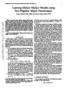
q is split into two new states q1 and q2 as depicted in Fig. 8. The input states i1 , . . . , ik and output states o1 , . . . , ol are those directly connected to q in the current model12 , in which all transition probabilities A are known. The topology after splitting provides additional degrees of freedom in the transition probabilities. The new transition probabilities x, y, z form the variables of an optimization problem, which can be represented by the matrices X (k × 2), Y (2 × l) and Z (2 × 2). The objective function to be minimized measures with respect to the target MFPT: P|Σ| a leastˆ squares error 2 W (X, Y, Z) = i,j=1, i6=j (Mij − Mij //κ) , where Mij //κ is computed according to definition 14. The best model according to the log-likelihood value is selected and the process is iterated till convergence of the log-likelihood function.
Solving the optimization problem The following constraints are used during the optimization of MFPT in a new candidate model. The first set of constraints ensures that the model remains a proper POMM: all transition probabilities must remain between 0 and 1 (C.1) and the outgoing probability mass from any state must sum up to 1 (C.2). 0 ≤ xj1 , xj2 ≤ 1 j = 1, . . . , k 0 ≤ y1i , y2i ≤ 1 i = 1, . . . , l 0 ≤ z11 , z12 , z21 , z22 ≤ 1 Pl y + z11 + z12 = 1 Plj=1 1j j=1 y2j + z21 + z22 = 1 xj1 + xj2 = Aij q j = 1, . . . , k
(C.1)
(C.2)
The second set of constraints guarantees that the stationary distribution of P the blocks is preserved. The input stream to a state q is defined as ISq = q 0 ∈Q πq 0 Aq 0 q and the stationary distribution can be formulated as πq = ISq . If the input stream to an output state oj is preserved then πoj remains 1−Aqq unchanged since Aoj oj is constant. By induction, if the input stream to each output state is preserved, the stationary distribution of every state different from q1 and q2 is unchanged. Consequently, the stationary distribution of every block but κq (the block containing q1 and q2 ) remains unchanged. As the stationary distribution of the blocks sums up to 1, πκq is then necessarily preserved and πq1 + πq2 = πq . Preserving the input streams to output states is formulated as follows: 12
Input and output states are not necessarily distinct.
20
INGI Research Report No. 2005-09
πq1 y1i + πq2 y2i = πq Aqoi , ∀i = 1, . . . , l where the stationary distribution vector π is obtained by solving the linear system given in definition 8. The optimization problem is non-linear both in the objective function and the constraints (as πq1 and πq2 depend on the problem variables). This problem can be solved using a Sequential Quadratic Programming (SQP) method [Fletcher, 1987]. In our experiments, we used the SQP solver provided in the Matlab optimization toolbox. This method requires the derivation of the objective function with respect to the problem variables. The objective function is derived hereafter with respect to a generic variable γ which can be instantiated to any x, y or z: |Σ| X ∂W (X, Y, Z) ˆ ij − Mij //κ) ∂Mij //κ = −2 (M ∂γ ∂γ i,j=1, i6=j
According to definition 14, the derivative of Mij //κ is given by ! κ 1 X ∂πq κj ∂wq j ∂Mij //κ = w + πq ∂γ πκj q∈κ ∂γ q ∂γ i
The linear system related to the stationary distribution introduced in definition 8 can be rewritten as (AT − I)π = 0. Therefore, the derivative of the stationary distribution can be obtained by solving the following system: (AT − I)
∂AT ∂π =− π ∂γ ∂γ
This derivation is straightforward as the only matrix to differentiate symbolically is AT . According to definition 13, the derivative of the MTA vector is κj ∂Nκ given by ∂ w = ∂γ j 1. It depends on the derivative13 of the fundamental ∂γ matrix Nκj = (I − Aκj )−1 where κj = Q \ κj : ∂Nκj ∂Aκj = Nκ j Nκ j ∂γ ∂γ Finally, the symbolic differentiation of the transition matrix A (or a sub∂A matrix of A) is made component-wise: ∂γij = 1 if Aij = γ and 0 otherwise. Two possible numerical difficulties might be encountered during the optimization procedure. When all the input (output) transitions to (from) a state 13
The derivative of an inverse matrix B −1 is given by:
∂B −1 ∂γ
−1 = −B −1 ∂B . ∂γ B
Learning Hidden Markov Models to Fit Long-Term Dependencies
21
are close to 0, the matrices (I − Aκj ) are nearly singular as the model nearly becomes unconnected. In order to avoid this problem, variable updates must be kept small enough. In addition, the inabililty of numerical solvers to set variables exactly to their bounds is an important issue for structural induction. Indeed, if the solver cannot set transition probabilities to 0, each split results in the full topology displayed in figure 8. While it is possible to cut transitions that are below a given threshold, we propose to use the Lagrange multiplier in order to detect the active box constraints (C.1). According to the solver precision, a Lagrange multipliers is different from 0 when the corresponding constraint is active, i.e. the current solution is on the constraint. At the end of the optimization procedure, the variables with an active box constraint are set to their corresponding bound value (0 or 1).
7
Experiments
In order to report comparative performances of the proposed approach in a controlled setting, a set of target models including long term dependencies were randomly generated. The target POMM on the left of Figure 7 is a typical example. Some states include a self loop transition with a high probability (θ > 0.5) such as the states labeled d in this example. These states are called short-term as the prediction of the next symbol d given previous d’s depends on a short history. Other states, called long-term, emit a specific letter not found elsewhere in the model (such as the states labeled e and f in this example) based on an unbounded history. A target model is initially generated so as to alternate short-term and long-term states in a cyclic fashion. The self-loop transition probability was fixed to θ = 0.65 in our experiments. This random generation gives rise to a transition matrix A1 . In order to deal with a sufficiently general class of target models, this transition matrix is interpolated with a random primitive stochastic matrix: A ← 0.9A1 + 0.1Arand . The resulting models are thus fully connected with a tendency to include long term dependencies. As pairs of short term states were chosen to emit the same letter, the relation between the alphabet size and the number of states is here |Σ| = 34 |Q|. Test samples contain 100 sequences of length 1,000 which were randomly generated from each target model. The test perplexity of each induced model is reported below as a relative increase with respect to the target model perplexity on the same test samples. Perplexity (PP) is related to the per symbol log-likelihood and formally defined as: 1
P P = 2− ||S||
P
x∈S
log2 P (x|T )
22
INGI Research Report No. 2005-09
where ||S|| denotes the total number of letters in the sample S and P (x|T ) denotes the probability of generating the string x from the model T . Perplexity can be interpreted as a measure of the average uncertainty for predicting the next symbol at any given position in the test strings. An uninformed model would predict any symbol of the alphabet Σ with the same probability 1/|Σ|. Such a model would have P P = |Σ|. The better a model fits a target distribution, the lower the perplexity. Figure 9 reports the learning curves obtained on average over 4 different target model sizes. For each target model, results are averaged over 10 learning sequences of growing length and independently drawn from each target model. We compare here the proposed POMM induction algorithm with EM estimation (i.e. Baum-Welch) of fully connected HMMs and trigram models. EM estimation is repeated with 3 different random initializations of the parameter values and the performance is reported only for the best model, which offers the highest likelihood of the training sample. Moreover BaumWelch is iterated with fully connected HMMs of growing number of states as long as the training sample likelihood significantly increases. Only the best performances of this approach are reported here. Both POMMs and HMMs are smoothed by defining a 10−6 minimal probability for any letter in any context and renormalizing the model accordingly. Trigrams are smoothed with a much more sophisticated technique known as the modified back-off scheme [Kneser and Ney, 1995]. This model is equivalent to a variable order Markov chain due to the back-off to lower order estimates. POMM induction via state splitting always performs better than competing techniques. In particular, good performances are obtained typically with learning sequences of size 2,000 while Trigrams and EM estimation generally require more data. With such a sample size the test perplexity increase relative to the target model falls between 3 and 10 % depending on the model size. This perplexity increase goes up to 35 % for EM trained models. Trigrams offer intermediate performances. Note that the Trigram quality is most likely due to its specific smoothing technique which compensates for the short-term model structure. In our current implementation, induction from a sequence of length 1,000, generated from a target model containing 16 states, takes a few seconds for Trigrams, about 36 minutes for EM estimation and 50 minutes for POMMStateSplit on a standard PC.
8
Conclusion
We propose in this paper a novel approach to the induction of the structure of Hidden Markov Models. The notion of partially observable Markov models
Learning Hidden Markov Models to Fit Long-Term Dependencies Target size = 4 Alphabet size = 3 0.25
Target size = 8 Alphabet size = 6 0.5
EM Trigram POMMStateSplit
EM Trigram POMMStateSplit
0.45 0.4 Perplexity increase
0.2 Perplexity increase
23
0.15
0.1
0.05
0.35 0.3 0.25 0.2 0.15 0.1 0.05
0
0 500
1000
1500
2000 2500 3000 3500 4000 Size of the learning sequence
4500
5000
500
1000
Target size = 16 Alphabet Size = 12 0.4
4500
5000
EM Trigram POMMStateSplit
0.6
Perplexity increase
0.3 Perplexity increase
2000 2500 3000 3500 4000 Size of the learning sequence
Target size = 32 Alphabet size = 24 0.7
EM Trigram POMMStateSplit
0.35
1500
0.25 0.2 0.15 0.1
0.5 0.4 0.3 0.2 0.1
0.05 0
0 500
1000
1500
2000 2500 3000 3500 4000 Size of the learning sequence
4500
5000
500
1000
1500
2000 2500 3000 3500 4000 Size of the learning sequence
4500
5000
Figure 9: Test perplexity increase (relative to the target model perplexity) with respect to the size of the learning sequence. The plots include 1 standard deviation intervals computed over 10 learning sequences in each case. (POMMs) is introduced. POMMs form a particular case of HMMs where any state emits a single letter with probability one, but several states can emit the same letter. It is shown that any HMM can be represented by an equivalent POMM. The induced model is constructed to fit the dynamics of the target machine, that is to best approximate the stationary distribution and the mean first passage times (MFPT) observed in the sample. HMMs are able to model a broader class of distributions than finite order Markov chains. They are well suited to represent in a compact way long term probabilistic dependencies. Accurate modeling of these dependencies cannot be achieved however through the classical approach of Baum-Welch estimation of a fully connected model. These observations motivate the use of MFPT to guide the search of an appropriate model topology. The proposed induction algorithm relies on non-linear optimization and iterative state splitting from an initial order one Markov chain. Experimental results illustrate the advantages of the proposed approach as compared to Baum-Welch HMM estimation or back-off smoothed Ngrams. Our future work includes extension of the proposed approach to other classes of models, such as lumped processes of periodic or absorbing Markov chains. The current implementation of our induction algorithm considers all
24
INGI Research Report No. 2005-09
states of the current model as candidates for splitting. More efficient ways of selecting the best state to split at any given step are under study. Applications of the proposed approach to larger datasets will also be considered, typically in the context of language or biological sequence modeling.
Acknowledgment The authors wish to thank Philippe Delsarte for many fruitful discussions about this work. This work is partially supported by the Fonds pour la formation `a la Recherche dans l’Industrie et dans l’Agriculture (F.R.I.A.) under grant reference F3/5/5-MCF/FC-19271.
References [Bengio and Frasconi, 1995] Bengio, Y. and Frasconi, P. (1995). Diffusion of context and credit information in markovian models. Journal of Artificial Intelligence Research, 3:223–244. [Callut and Dupont, 2004] Callut, J. and Dupont, P. (2004). A Markovian approach to the induction of regular string distributions. In Grammatical Inference: Algorithms and Applications, number 3264 in Lecture Notes in Artificial Intelligence, pages 77–90, Athens, Greece. Springer Verlag. [Carrasco and Oncina, 1999] Carrasco, R. and Oncina, J. (1999). Learning deterministic regular gramars from stochastic samples in polynomial time. Theoretical Informatics and Applications, 33(1):1–19. [Denis and Esposito, 2004] Denis, F. and Esposito, Y. (2004). Learning classes of probabilistic automata. In Proc. of 17th Annual Conference on Learning Theory (COLT), number 3120 in Lecture Notes in Computer Science, pages 124–139, Banff, Canada. Springer Verlag. [Dupont and Amengual, 2000] Dupont, P. and Amengual, J. (2000). Smoothing probabilistic automata: an error-correcting approach. In Oliveira, A., editor, Grammatical Inference: Algorithms and Applications, number 1891 in Lecture Notes in Artificial Intelligence, pages 51–64, Lisbon, Portugal. Springer Verlag. [Dupont and Chase, 1998] Dupont, P. and Chase, L. (1998). Using symbol clustering to improve probabilistic automaton inference. In Grammatical Inference, ICGI’98, number 1433 in Lecture Notes in Artificial Intelligence, pages 232–243, Ames, Iowa. Springer Verlag.
Learning Hidden Markov Models to Fit Long-Term Dependencies
25
[Dupont et al., 2005] Dupont, P., Denis, F., and Esposito, Y. (2005). Links between Probabilistic Automata and Hidden Markov Models: probability distributions, learning models and induction algorithms. Pattern Recognition, 38(9):1349–1371. [Durbin et al., 1998] Durbin, R., Eddy, S., Krogh, A., and Mitchison, G. (1998). Biological sequence analysis. Cambridge University Press. [Fletcher, 1987] Fletcher, R. (1987). Practical Methods of Optimization, chapter 8.7 : Polynomial time algorithms, pages 183–188. John Wiley & Sons, New York, second edition. [Freitag and McCallum, 1999] Freitag, D. and McCallum, A. (1999). Information extraction with HMMs and shrinkage. In Proc. of the AAAI-99 Workshop on Machine Learning for Information Extraction. [Freitag and McCallum, 2000] Freitag, D. and McCallum, A. (2000). Information extraction with HMM structures learned by stochastic optimization. In Proc. of the Seventeenth National Conference on Artificial Intelligence, AAAI, pages 584–589. [Kemeny and Snell, 1983] Kemeny, J. and Snell, J. (1983). Finite Markov Chains. Springer-Verlag. [Kermorvant and Dupont, 2002] Kermorvant, C. and Dupont, P. (2002). Stochastic grammatical inference with multinomial tests. In Adriaans, P., Fernau, H., and van Zaanen, M., editors, Proceedings of the 6th International Colloquium on Grammatical Inference: Algorithms and Applications, number 2484 in Lecture Notes in Artificial Intelligence, pages 149–160, Amsterdam, the Netherlands. Springer Verlag. [Kneser and Ney, 1995] Kneser, R. and Ney, H. (1995). Improved backing-off for m-gram language modeling. In International Conference on Acoustic, Speech and Signal Processing, pages 181–184, Detroit, Michigan. [Levin and Pieraccini, 1993] Levin, E. and Pieraccini, R. (1993). Planar Hidden Markov modeling: from speech to optical character recognition. In Giles, C., Hanton, S., and Cowan, J., editors, Advances in Neural Information Processing Systems, volume 5, pages 731–738. Morgan Kauffman. [Llorens et al., 2002] Llorens, D., Vilar, J.-M., and Casacuberta, F. (2002). Finite state language models smoothed using n-grams. International Journal of Pattern Recognition and Artificial Intelligence, 16(3):275–289.
26
INGI Research Report No. 2005-09
[Meyer, 2000] Meyer, C. D. (2000). Matrix analysis and applied linear algebra. Society for Industrial and Applied Mathematics. [Norris, 1997] Norris, J. R. (1997). Markov Chains. Cambridge University Press, United Kingdom. [Ostendorf and Singer, 1997] Ostendorf, M. and Singer, H. (1997). HMM topology design using maximum likelihood successive state splitting. Computer Speech and Language, 11:17–41. [Rabiner and Juang, 1993] Rabiner, L. and Juang, B.-H. (1993). Fundamentals of Speech Recognition. Prentice-Hall. [Ron et al., 1994] Ron, D., Singer, Y., and Tishby, N. (1994). Learning probabilistic automata with variable memory length. In Proceedings of the Seventh Annual Conference on Computational Learning Theory, New Brunswick, NJ. ACM Press. [Rulot and Vidal, 1988] Rulot, H. and Vidal, E. (1988). An efficient algorithm for the inference of circuit-free automata. In Ferrat`e, G., Pavlidis, T., Sanfeliu, A., and Bunke, H., editors, Advances in Structural and Syntactic Pattern Recognition, pages 173–184. NATO ASI, Springer-Verlag. [Senata, 1981] Senata, E. (1981). Non-negative Matrices and Markov Chains. Springer-Verlag. [Stolcke, 1994] Stolcke, A. (1994). Bayesian Learning of Probabilistic Language Models. Ph. D. dissertation, University of California. [Thollard et al., 2000] Thollard, F., Dupont, P., and de la Higuera, C. (2000). Probabilistic DFA Inference using Kullback-Leibler Divergence and Minimality. In Seventeenth International Conference on Machine Learning, pages 975–982. Morgan Kauffman.