School of Computing Science, Simon Fraser University, Vancouver, B.C., Canada. {zza27, li, mark}@cs.sfu.ca. ABSTRACT. In this paper, we propose a novel ...
LEARNING IMAGE SIMILARITIES VIA PROBABILISTIC FEATURE MATCHING Ziming Zhang,
Ze-Nian Li,
Mark S. Drew
School of Computing Science, Simon Fraser University, Vancouver, B.C., Canada {zza27, li, mark}@cs.sfu.ca ABSTRACT In this paper, we propose a novel image similarity learning approach based on Probabilistic Feature Matching (PFM). We consider the matching process as the bipartite graph matching problem, and define the image similarity as the inner product of the feature similarities and their corresponding matching probabilities, which are learned by optimizing a quadratic formulation. Further, we prove that the image similarity and the sparsity of the learned matching probability distribution will decrease monotonically with the increase of parameter C in the quadratic formulation where C ≥ 0 is a pre-defined datadependent constant to control the sparsity of the distribution of a feature matching probability. Essentially, our approach is the generalization of a family of similarity matching approaches. We test our approach on Graz datasets for object recognition, and achieve 89.4% on Graz-01 and 87.4% on Graz-02, respectively on average, which outperform the stateof-the-art. Index Terms— Similarity Learning, Probabilistic Feature Matching, Object Recognition 1. INTRODUCTION Similarity-based methods have proven effective in many computer vision tasks, in particular object recognition in images. A natural way to measure image similarity is to match their features, and two images should be deemed similar if many of the features in one image have matching features in the other. In this paper, we consider each image as an undirected graph and take the feature matching process as the bipartite graph matching problem as illustrated in Fig. 1, which indicates that any pair of features from two images could be possibly matched. Note that this matching process could be easily extended to other types of data, not restricted to images. Different strategies can be utilized in the feature matching process. Lyu [1] introduced a Summation Kernel (SK) to measure the image similarity as follows: X X Ksum (V1 , V2 ) = k(vi , vj ) (1) vi ∈V1 vj ∈V2
where V1 (resp. V2 ) denotes a feature set, vi ∈ V1 (resp. vj ∈ V2 ) denotes a feature vector in V1 (resp. V2 ), and
Fig. 1. Illustration of matching two images. Each image is represented as a collection of features of the patches. Weights (red) on the edges (green), denote the matching probabilities between the feature pairs so that the similarity between the two images is obtained. This figure is best viewed in color.
k(vi , vj ) denotes an arbitrary feature similarity kernel. In the next sections, we denote k(vi , vj ) as kij for short. Wallraven et al. [2] proposed a Max-selection Kernel (MK) as shown below: X X 1 (2) Kmax (V1 , V2 ) = max kji max kij + vj ∈V2 vi ∈V1 2 vi ∈V1
vj ∈V2
Fr¨ohlich et al. [3] proposed the Optimal Assignment Kernel (OAK) to maximize the similarity score between two structured objects by finding exactly one-to-one matches between the parts of these objects, defined as follows: ( P|x| maxπ i=1 k(xi , yπ(i) ) if |y| > |x| P|y| KOA (x, y) = (3) maxπ j=1 k(xπ(j) , yj ) otherwise where x (resp. y) denotes an object, xi (resp. yj ) denotes a part of x (resp. y), |x| (resp. |y|) denotes the number of the parts of x (resp. y), and π denotes a permutation of parts. In contrast, the novel contribution of this paper is that we introduce a probabilistic matching strategy in the matching process as illustrated in Fig. 1, and further propose a novel similarity learning approach as a generalization of a family of similarity learning approaches, including SK, MK, and OAK,
such that the similarity measure can be decided adaptive to data. In our approach, the similarity between two images is defined as the inner product of their feature similarities and the corresponding feature matching probabilities, which are learned by optimizing a quadratic formulation. The rest of the paper is organized as follows. Section 2 explains our approach in detail. Section 3 shows our experimental results for object recognition in images. We conclude the paper in Section 4. 2. PROBABILISTIC MATCHING BASED SIMILARITY LEARNING Given two images X={x1 , · · · , x|X| } and Y ={y1 , · · · , y|Y | }, where xi ∈ X (resp. yj ∈ Y ) denotes a feature in X (resp. Y ) and |X| (resp. |Y |) denotes the number of features in X (resp. Y ), according to the bipartite graph matching problem, their similarity can be defined as follows: S(X, Y ; α, k) =
|X| |Y | X X
αij kij
(4)
i=1 j=1
where αij denotes the feature matching probability (FMP) between features xi and yj , kij denotes their similarity, and S(X, Y ; α, k) denotes the similarity between X and Y given the feature matching probability function α (see Section 2.1 for details) and their feature similarity matrix k. 2.1. Feature Matching Probability Function Intuitively, an FMP αij can be utilized to describe how likely feature xi and yj are matched. As illustrated in Fig. 1, the axle with black circle on the left has 0.8 FMP with the axle with black circle on the right, while it has 0.2 FMP with the background feature, which is quite reasonable. Notice that a meaningful FMP should be a non-negative relative measurement with normalization. Thus, the total probabilities of the matching pairs should be equal to the smaller number of features between two images. This constraint makes sure that every feature with the fewer amount will find probabilistic matches. Therefore, by considering the matching process as a function, we give its definition as follows: Definition (Feature Matching Probability Function). Given two images X={x1 , · · · , x|X| } and Y ={y1 , · · · , y|Y | }, a feature matching probability function (FMPF) α is defined as α : X × Y → {R− }|X|×|Y | , where R− denotes a non− − negative real number. Letting → x and → y denote the two dimensions of α, and selecting an arbitrary dimension set − − H ⊆ {→ x,→ y } from α, each FMPF will correspond to a point in the vector space covered by the following convex set: X X α| α � 1, αij = min (|X|, |Y |) , 0 � α � 1 ∀h∈H
i,j
where “�” denotes the element-wise operator of “≤”. Notice that if H = ∅, the first constraint in the convex set above does not apply. 2.2. Probabilistic Feature Matching Learning We would like to perform the probabilistic feature matching between two images automatically. Therefore, we propose a quadratic optimization formulation [4] as defined in Eqn. 5 to calculate α, where f (α; C) denotes our objective function, α is the only variable, C ≥ 0 is a pre-defined non-negative constant, and k is the feature similarity matrix. X X 2 max f (α; C) = αij kij − C αij (5) α
i,j
s.t.
X ∀h∈H
α � 1,
X
i,j
αij = min (|X|, |Y |) , 0 � α � 1
i,j
In order to see the relationship between our approach and some other similarity learning approaches, we need the following important theorems on convexity [4]: Theorem 1. Consider max f (x) over x ∈ X , where f (x) is convex, and X is a closed convex set. If the optimum exists, a boundary point of X is the optimum. Theorem 2. If a convex function f (x) attains its maximum on a convex polyhedron X with some extreme points, then this maximum is attained at an extreme point of X . Based on the theorems above, we can show that in certain cases our approach can be considered as equivalences to some particular approaches by choosing different C and H. − − • C = +∞ and H = {→ x,→ y }: According to Thm. 1, the learned α will be a uniform distribution, that is, 1 αij = max(|X|,|Y |) , and by normalizing α, our learned similarity is equivalent to the SK [1] approach. − − • C = 0 and H = {→ x,→ y }: According to Thm. 2, the learned α will simulate a one-to-one matching process, and the learned similarity is equivalent to the OAK [3] approach. − • C = 0 and H = {→ x }: According to Thm. 2, the learned α will simulate the matching process that se− lects the biggest similarity along the → x -dimension for → − each feature in the y -dimension, and the learned simP ilarity is equivalent to vj ∈V2 maxvi ∈V1 kji in Eqn. 2. − − Thus, by learning α along the → x - and → y -dimension, respectively, our approach is equivalent to the MK [2] approach. Moreover, our approach has the following property: Proposition. For two images X and Y , both the sparseness of α and their similarity S(X, Y ; α, k) will decrease monotonically with increasing C in Eqn. 5.
Proof. Considering C1 > C2 ≥ 0 and their corresponding α1 and α2 calculated using Eqn. 5, we have f (α1 ; C1 ) ≥ f (α2 ; C1 ) and f (α2 ; C2 ) ≥ f (α1 ; C2 ). Putting them together, we have C1 α20 α2 −C1 α10 α1 ≥ α20 k−α10 k ≥ C2 α20 α2 −C2 α10 α1 (6) where α1 , α2 and k are vectorized, and 0 denotes the transpose operator. Then we get (C1 − C2 )(α20 α2 − α10 α1 ) ≥ 0
(7)
Since C1 > C2 ≥ 0, then α10 α1 ≤ α20 α2 , which indicates that a smaller C will lead to an α with larger sparseness. Besides, we have S(X, Y ; α2 , k) − S(X, Y ; α1 , k) = α20 k − α10 k ≥ C2 (α20 α2 − α10 α1 ) ≥ 0
(8)
Therefore, S(X, Y ; α, k) will decrease monotonically with the increase of C. This property simplifies the adjustment of C in the crossvalidation for different data so that our approach can be adaptive to the data. 2.3. Classification with Support Vector Machines In general, there is no guarantee that the similarity matrix generated by our approach is a valid kernel, whereas theoretically support vector machines (SVMs) are utilized with kernels for classification. However, in practice, an arbitrary similarity matrix can be involved in an SVM by adding a small positive number to the entries along the diagonal when it is not valid, as did in Eqn. 9, where |λmin | denotes the absolute value of the minimum eigenvalue of the similarity matrix K, and I denotes the identity matrix. K 0 = K + |λmin |I,
if λmin < 0
(9)
3. EXPERIMENTS We tested our approach on Graz-01 [5] and Graz-02 [6] datasets to perform the “object & non-object” binary classification, with performance measured by Equal Error Rate (EER). Graz-01 is a challenging dataset with two object categories (bike: 373 images, person: 460 images) and a background category (270 images), because they vary greatly in object scale, pose and illumination. Compared to Graz-01, Graz-02 can be considered as an improved version with much more challenge, and comprises 3 object categories (bike: 365 images, person: 311 images, car: 420 images) and a background category (380 images). The size of each image in both datasets is either 640×480 or 480×640 pixels. In our experiments, all the images were converted into gray scale, and we utilized the dense sampling technique [7]
to sample the images so that each patch consists of 10×10 pixels. For each patch, we employed the SIFT [8] descriptor to represent it, and then used k-means to generate a codebook with 200 codewords so that each descriptor can be represented by the closest codeword in the feature space. Finally, by counting the occurrence of each codeword in the cells of the 3×3 grid, we created 9 histograms to represent each image. The RBF-kernel with χ2 distance measurement was used to compare the similarity of two histograms, that is, ) ( d X (vi,n − vj,n )2 (10) kij = exp − vi,n + vj,n n=1 where d is the number of dimensions of histograms vi and vj . The penalty parameter in SVM was fixed to 104 . All the results here were averaged after 50 runs. To simplify the notations, we use PFM1 , PFM2 and PFM3 to denote our approach − − − − with H = {→ x,→ y }, H = {→ x } or H = {→ y }, and H = ∅, respectively. 3.1. Graz-01 For the training-test data selection, we followed the setup in [9]. Specifically, we randomly selected 100 images in the positive class and 50 in each negative class (including the background) as our training set, and performed the test on similarly distributed data sets consisting of half the number of the training images per category. Fig. 2 shows our performance on Graz-01. In general, PFM1 performs best, while PFM3 performs worst, and PFM1 is much more stable with the increase of C than the other two, but there is no evidence that indicates what is the best C for this dataset. We also list the best performance of each PFM in Table 1 and compare them with other state-of-the-art results. Clearly, all of our results outperform the others. Table 1. Comparison results between different approaches on Graz-01 (%) SPK [9] PDK [10] PFM1 (C=0) PFM2 (C=5) PFM3 (C=+∞)
Bike 86.3±2.5 90.2±2.6 90.6±5.3 89.6±4.9 89.6±4.8
Person 82.3±3.1 87.2±3.8 88.2±4.6 88.5±4.6 87.9±5.1
Ave. 84.3 88.7 89.4 89.0 88.8
3.2. Graz-02 We followed the experimental setup in [6] for the training-test data selection. Specifically, for each object category, we randomly selected 150 positive and 150 negative (50 for each non-object class, including the background) images as the training data, and selected 75 positive and 75 negative (25 for each non-object class, including the background) with similar distribution of the training data as the test data, respectively.
→ → (a) PFM1 (with H = {− x ,− y })
→ → (b) PFM2 (with H = {− x } or H = {− y })
(c) PFM3 (with H = ∅)
Fig. 2. Performance comparison on Graz-01 dataset between different PFM with different C.This figure is best viewed in color.
→ → (a) PFM1 (with H = {− x ,− y })
→ → (b) PFM2 (with H = {− x } or H = {− y })
(c) PFM3 (with H = ∅)
Fig. 3. Performance comparison on Graz-02 dataset between different PFM with different C.This figure is best viewed in color. Fig. 3 shows our performance on Graz-02. Compared to Fig. 2, similar observations can be made. Therefore, H = − − {→ x,→ y } seems the best choice among the three for our PFM. Also, Table 2 lists the best results using different PFM in comparison with some other state-of-the-art results, and all of ours outperform the others significantly.
a family of similarity measurement approaches, including the Optimal Assignment Kernel, the Max-selection Kernel, and the Summation Kernel. In our experiments, we tested our approach on Graz datasets for object recognition, and our results outperformed the state-of-the-art. On average, we achieved 89.4% on Graz-01 and 87.4% on Graz-02, respectively. 5. REFERENCES
Table 2. Comparison results between different approaches on Graz-02 (%) Boost.+SIFT [6] Boost.+Comb. [6] PDK+SIFT [10] PDK+hybrid [10] PFM1 +SIFT (C=5) PFM2 +SIFT (C=10) PFM3 +SIFT (C=+∞)
Bike 76.0 77.8 86.7 86.0 88.9 88.0 87.7
Person 70.0 81.2 86.7 87.3 88.1 87.9 87.8
Car 68.9 70.5 74.7 74.7 85.2 83.6 82.6
Ave. 71.6 76.5 82.7 82.7 87.4 86.5 86.0
4. CONCLUSION In this paper, we propose a novel image similarity learning approach based on Probabilistic Feature Matching (PFM). In our approach, the similarity between two images is defined as the inner product between the feature similarities and their corresponding matching probabilities, which are learned datadependently by solving a quadratic optimization problem. We also prove that the image similarity and the sparsity of the feature matching probability distribution will decrease monotonically with the increase of parameter C in the quadratic formulation. Essentially, our approach is the generalization of
[1] S.W. Lyu, “Mercer kernels for object recognition with local features,” in CVPR’05, 2005, pp. II: 223–229. [2] C. Wallraven, B. Caputo, and A. Graf, “Recognition with local features: the kernel recipe,” in ICCV’03, 2003, pp. 257–264. [3] Holger Fr¨ohlich, J¨org K. Wegner, Florian Sieker, and Andreas Zell, “Optimal assignment kernels for attributed molecular graphs,” in ICML’05, 2005, pp. 225–232. [4] K.G. Murty, Linear Complementarity, Linear and Nonlinear Programming, Helderman-Verlag, Berlin, 1988. [5] A. Opelt, M. Fussenegger, A. Pinz, and P. Auer, “Weak hypotheses and boosting for generic object detection and recognition,” in ECCV’04, 2004, pp. Vol II: 71–84. [6] A. Opelt, A. Pinz, M. Fussenegger, and P. Auer, “Generic object recognition with boosting,” PAMI, vol. 28, no. 3, pp. 416–431, March 2006. [7] K. E. A. van de Sande, T. Gevers, and C. G. M. Snoek, “Evaluating color descriptors for object and scene recognition,” PAMI, 2010. [8] David G. Lowe, “Object recognition from local scale-invariant features,” in ICCV’99, 1999. [9] Svetlana Lazebnik, Cordelia Schmid, and Jean Ponce, “Beyond bags of features: Spatial pyramid matching for recognizing natural scene categories,” in CVPR’06, 2006, pp. 2169–2178. [10] H.B. Ling and S. Soatto, “Proximity distribution kernels for geometric context in category recognition,” in ICCV’07, 2007.