Learning in Games with Unstable Equilibria∗ Michel Benaïm† Institut de Mathématiques Université de Neuchâtel CH-2007 Neuchâtel, Switzerland
Josef Hofbauer‡ Department of Mathematics University College London London WC1E 6BT, UK
Ed Hopkins§ Economics University of Edinburgh Edinburgh EH8 9JY, UK December, 2005 Abstract We propose a new concept for the analysis of games, the TASP, which gives a precise prediction about non-equilibrium play in games whose Nash equilibria are mixed and are unstable under fictitious play-like learning processes. We show that, when players learn using weighted stochastic fictitious play and so place greater weight on more recent experience, the time average of play often converges in these “unstable” games, even while mixed strategies and beliefs continue to cycle. This time average, the TASP, is related to the best response cycle first identified by Shapley (1964). Though conceptually distinct from Nash equilibrium, for many games the TASP is close enough to Nash to create the appearance of convergence to equilibrium. We discuss how these theoretical results may help to explain data from recent experimental studies of price dispersion.
Journal of Economic Literature classification numbers: C72, C73, D83. Keywords: Games, Learning, Best Response Dynamics, Stochastic Fictitious Play, Mixed Strategy Equilibria, TASP. ∗
We thank Tilman Börgers, Tim Cason, Dan Friedman, Martin Hahn, Larry Samuelson, Bill Sandholm, Sylvain Sorin and Jörgen Weibull for helpful comments. †
[email protected], http://www.unine.ch/math/personnel/equipes/benaim/benaim_pers/benaim.html; Michel Benaïm thanks the Swiss National Science Foundation for support, Grant 200021-1036251/1. ‡
[email protected], http://homepage.univie.ac.at/Josef.Hofbauer/; Josef Hofbauer thanks ELSE for support. § Corresponding author:
[email protected], http://homepages.ed.ac.uk/ehk/; Ed Hopkins thanks the Economic and Social Research Council for support, award reference RES-000-27-0065.
1
Introduction
At the basis of the theory of learning in games is the question as to whether Nash equilibria are stable or unstable. The hope is to predict play: if an equilibrium is an attractor for a plausible learning dynamic, we think that it is a possible outcome for actual play. However, testing such a prediction is complicated by the fact that there are several measures of whether play is at or near an equilibrium. Particularly, for mixed Nash equilibria, as players’ mixed strategies are not directly observable, necessarily in empirical work researchers must look at play averaged over a number of periods, at least as a first approximation. On the other hand, if a Nash equilibrium is unstable, we would expect actual players, for example, subjects in an experiment, not to play that equilibrium or even to be close to it. Shapley (1964) famously found that there are games for which learning may not approach the only Nash equilibrium but rather will continuously cycle. If we take this result seriously as an empirical prediction, then there are games in which Nash equilibrium play will never emerge. Note that as Shapley’s result also holds for average play, even average play should not be close to an unstable equilibrium. In this paper, we advance the novel hypothesis that even when learning diverges from equilibrium, it is still possible to make a precise prediction about play. Surprisingly, in games with a unique unstable mixed equilibrium the time average of play may converge even when players’ mixed strategies do not. If an equilibrium is unstable under stochastic fictitious play with the classical assumption that players place an equal weight on all past experience, then both mixed strategies and time averages must diverge from equilibrium. But we find that if greater weight is placed on more recent experience, as it is in “weighted” stochastic fictitious play, then although the players’ mixed strategies will approach the cycle of the type found by Shapley, the time average will converge. We show that, as the level of noise and the level of forgetting approach zero, the time average of play approaches the TASP (Time Average of the Shapley Polygon), that is, the time average of the Shapley cycle under the continuous time best response dynamics. We find that in many cases the TASP is close to the Nash equilibrium. Since the time average is much easier to observe than mixed strategies, it may well appear that play has converged to the equilibrium. We go on to identify games where the TASP and Nash equilibrium are quite distinct, and so offer the possibility of a clearer empirical test between the two. These results are not of purely theoretical interest. They, in fact, arise in direct response to recent experimental work on the economically important phenomenon of price dispersion. Cason and Friedman (2003) and Morgan, Orzen, and Sefton (2006) report on experimental investigations of the price dispersion models of Burdett and Judd (1983) and Varian (1980) respectively. Both studies report aggregate data that is remarkably close to the price distribution that would be generated if the subjects had been playing the mixed Nash equilibrium. This is surprising if one takes learning theory seriously, as earlier results by Hopkins and Seymour (2002) indicate that the mixed equilibria of these models are unstable under most common learning processes. 1
Cason, Friedman and Wagener (2005) reexamine the data from Cason and Friedman (2003) and indeed find that play is highly non-stationary and there are clear cycles present. They therefore reject the hypothesis that subjects were in fact playing Nash equilibrium. This is also consistent with the earlier results of Brown Kruse et al. (1994). They find, in an experimental study of a Bertrand-Edgeworth oligopoly market with no pure equilibrium, that prices cycle but prices averaged across the whole session still approximate the mixed equilibrium distribution. Our results explain the apparent empirical paradox. When mixed equilibria are unstable under learning, we predict persistent cycles in play. Nonetheless, if players learn placing more weight on recent experience, the time average of play should converge to the TASP, which in these games is close to the Nash equilibrium. It is true that there are existing results in evolutionary game theory that show convergence of time averages without convergence to equilibrium. For example, the evolutionary replicator dynamics cycle around mixed strategy equilibria of zero sum games, but the time average of the dynamics nonetheless converge (see, for example, Hofbauer and Sigmund (1998, pp120-130)). However, the current results are quite different. First, we obtain convergence in exactly the class of games where time averages do not converge under traditional assumptions. Second, the existing results show if that there is convergence of the time average of play, it must be to a Nash equilibrium. Here, we show convergence to the TASP which is distinct from both Nash equilibrium and perturbed equilibrium concepts such as quantal response or logit equilibrium. Fictitious play was introduced many years ago with the underlying principle that players play a best response to their beliefs about opponents, beliefs that are constructed from the average past play of opponents. This we refer to as players having “classical” beliefs. It was in this framework that Shapley (1964) obtained his famous result. However, even when fictitious play converges to a a mixed strategy equilibrium, it does so only in time average not in marginal frequencies. This problem motivated the introduction of smooth or stochastic fictitious play (see Fudenberg and Levine (1998) for a survey), which permits convergence in actual mixed strategies. This more recent work still employs classical beliefs. However, experimental work has found greater success with generalisations of fictitious play that allow for players constructing beliefs by placing greater weight on more recent events (see Cheung and Friedman (1997), Camerer and Ho (1999) amongst many others). This is called forgetting or recency or weighted fictitious play. Despite their empirical success, models with recency have not received much theoretical analysis, largely because they are more difficult to analyze than equivalent models with classical beliefs. This paper represents one of the few attempts to do so.1 Many years ago, Edgeworth (1925) predicted persistent cycles in a competitive situation where the only Nash equilibrium is in mixed strategies. This view was for a 1
There has been more work on fictitious play with finite memory, for example, Young (1993). Other learning models not based on fictitious play where the speed of learning does not decrease over time include Benaïm and Weibull (2003) and Hofbauer and Sandholm (2005).
2
long while superseded by faith that rational agents would play Nash equilibrium, no matter how complicated the model or market. In the case of mixed strategies, learning theory provides some support for Edgeworth, persistent cycles are a possibility even when agents have memory of more than the one period Edgeworth assumed (though in other games, learning will converge even to a mixed equilibrium). Furthermore, recent learning models that allow for stochastic choices do not imply the naive, predictable cycles described by Edgeworth. Cycles may only be detectable by statistical tests for non-stationarity (see Cason, Friedman and Wagener (2005)). In the absence of such sophisticated analysis, these perturbed Edgeworth-Shapley cycles may to an outside observer look indistinguishable from mixed equilibrium. Thus, while it is possible in principle to distinguish between the TASP and equilibrium play by testing for stationarity, it may not be easy. So, it would be convenient to have a simpler way of distinguishing between the two. We therefore construct some examples of games where the TASP and Nash equilibrium are quite distinct. These should make possible a simple test simply based on average play. We also find that the comparative statics of the TASP with respect to changes in payoffs differ from those of Nash equilibrium and of perturbed equilibrium concepts such as logit equilibrium. We are therefore optimistic that the theoretical results of this paper can and will be tested.
2
An Overview: Shapley Polygons and Edgeworth Cycles
We start with a generalisation of the well-known Rock-Scissors-Paper game and two specific examples, 0 RSP = b1 −a1
−a2 0 b2
b3 −a3 0
0 -1 3 A = 2 0 -1 -1 3 0
0 -3 1 B = 1 0 -2 -3 1 0
(1)
Game A and game B both have a unique Nash equilibrium in mixed strategies, for A, x∗ = (13, 10, 9)/32 = (0.40625, 0.3125, 0.28125) and, for B, x∗ = (9, 10, 13)/32 = (0.28125, 0.3125, 0.40625). They appear to be very similar. Learning theory, however, says that they are quite different. Specifically, if a single large population of players are repeatedly randomly matched to play one of these games, most learning and/or evolutionary dynamics, such as fictitious play, the replicator dynamics, reinforcement learning or stochastic fictitious play, should converge to (close to) the Nash equilibrium in game A, but should diverge from equilibrium in game B. Suppose we try to test this prediction experimentally. We assemble a group of subjects in a laboratory and we repeatedly match them randomly in pairs to play one of the two games. Now, mixed strategies are intrinsically hard to measure. So, suppose as a first approximation, we simply calculate the average frequency of each strategy 3
over the whole experimental session. The claim in the current paper is that, with sufficiently high monetary incentives, we would expect to see an average of approximately (0.41, 0.31, 0.28) in game A, and approximately (0.29, 0.34, 0.37) in game B. In the second game, play is not as close to Nash equilibrium as in the first, but since experimental data is usually fairly noisy, one might well conclude that this was a reasonable approximation, and convergence had taken place. This would of course lead one to reject the prediction of learning theory that play in the two games should be fundamentally different. What we find in this paper is that while learning behaviour in the two games is similar in terms of average frequencies, it will be quite different on other measures. Shapley (1964) was the first to show that there are games in which a learning process does not converge to a Nash equilibrium. Instead, the fictitious play process that he examined converged to a cycle of increasing length. We can recreate Shapley’s result in the context of a single large population who are repeatedly randomly matched in pairs to play a normal form game such as A or B above. Fictitious play assumes that agents play a best response given their beliefs. The vector xt represents the belief at time t, with xit the probability given to an opponent playing his i-th strategy. That is, xt ∈ S N P the simplex S N = {x = (x1 , ..., xN ) ∈ RN : xi = 1, xi ≥ 0, for i = 1, ..., N }. An agent then chooses a pure strategy that is in the set of best responses to her current beliefs, or b(xt ).2 The dynamic equation for the fictitious play process in a single population will be xt+1 − xt ∈ γ t (b(xt ) − xt ). (2) with γ t being the step size. Classically, beliefs are assumed to be based on the average of past play by their opponents, which implies that the step size will be equal to 1/(t + 1). An alternative, that is explored in this paper, is that players place a weight of one on last period’s observation, a weight δ on the previous period, and δ n−1 on their experience n periods ago, for some δ ∈ [0, 1). Then the step size γ t will be 1 − δ, a constant.
Suppose that δ takes the extreme value of 0, “Cournot beliefs”, so that players play a best response to the last choice of their opponent. In RSP, as Rock is the best response to Scissors which is the best response to Paper, we would see a cycle of the form P, S, R, P, S, R, P, S, R, .... This is a very simple example of an “Edgeworth cycle” of best responses. Clearly, if players follow this cycle the time average of their play will converge to (1/3, 1/3, 1/3). Of course, for some RSP games, this will be equal to or be close to the mixed Nash equilibrium. However, one would not describe this type of behaviour as equilibrium play, as it involves predictable cycles rather than randomisation. Or, more formally, there is only convergence of the time average, but not marginal frequencies. Under classical beliefs, change will be more gradual. For example, in the case of game B if beliefs are at a point to the right of A1 in Figure 1, where x1 is relatively high, 2
As b(·) is not in general single valued, the dynamics arising from fictitious play present certain mathematical difficulties. See Benaïm et al. (2005) for a full treatment.
4
x2 1
A r 2
£ £°
£
r
T s s
J ] J J
N
A3 XXX z
r
A1 0
1
0
x1
Figure 1: The Shapley triangle for game B with the TASP (T) and the Nash equilibrium (N). the best response will be the second strategy, or b(xt ) = e2 = (0, 1, 0). Agents in the population play the second strategy and beliefs about the likelihood of seeing strategy 2 increase. Beliefs move in the direction of the vertex where x2 = 1, until they approach near A2 , and strategy 3 becomes a best response. Then, beliefs will move toward the vertex e3 = (0, 0, 1) until strategy 1 becomes the best response. That is, there will be cyclical motion about the Nash equilibrium. In game A, it can be shown that over time the cycles converge on the Nash equilibrium, but in game B beliefs converge to the triangle A1 A2 A3 illustrated in Figure 1 and the cycles are persistent. The easiest way to prove such convergence results is to use the continuous time best response (BR) dynamics, defined as x˙ ∈ b(x) − x.
(3)
For a class of games including the game B given in (1), Gaunersdorfer and Hofbauer (1995) show that the best response dynamics converge to the “Shapley polygon” (Gilboa and Matsui (1991) use the term “cyclically stable set”). In game B this is the triangle A1 A2 A3 illustrated in Figure 1, but we can give a more general definition. 5
Definition 1 A Shapley polygon is a polygon in S N with M vertices A1 , ..., AM which is a closed orbit for the best response dynamics (3). We can then define the TASP as follows. Definition 2 The TASP (time average of the Shapley Polygon) is 1 x˜ = T
Z
0
T
1 b(x(t))dt = T
Z
T
x(t)dt
(4)
0
where x(0) = x(T ).3 That is, it is the time average of the best response dynamics (3) over one complete circuit of a Shapley polygon. In the standard case where the best replies along the cycle are pure strategies, it is possible to be more specific. We label an edge the ith edge if on that edge the ith strategy is being played. That is, on that edge, b(x) = ei , that is the vector with 1 at position i and zero elsewhere. Suppose that at some time t0 , the dynamics (3) are at vertex Ai−1 . Denote the coordinates of the ith vertex as xAi . Then, because between Ai−1 and Ai the best response b(x) is ei , the BR dynamics imply the linear differential A equation x˙ i = 1 − xi with initial condition xi (t0 ) = xi i−1 . Thus, we have on that edge A xi (t0 + t) = 1 + exp(−t)(xi i−1 − 1). Let Ti be the total time spent by the continuous Ai−1 i time BR dynamics on the ith edge. Or, let Ti solve xA − 1). i = 1 + exp(−Ti )(xi Then, over one complete circuit of the Shapley polygon, x˜i is the proportion of time spent on side i, or, Ti (5) x˜i = PM T j j=1 Now, Shapley polygons do not exist for every game. For example, in game A in (1) the Nash equilibrium is a global attractor for the best response dynamics and there is no Shapley polygon. But for the game B, there is a Shapley triangle (which is unique and asymptotically stable) and, following Gaunersdorfer and Hofbauer (1995), we can calculate that A1 = (6, 1, 3)/10, A2 = (2, 6, 1)/9, and A3 = (1, 3, 9)/13 as shown in Figure 1. The TASP can be computed numerically as x˜ ≈ (0.29, 0.34, 0.37), marked as “T” in Figure 1.
Benaïm et al. (2005) recently have extended the theory of stochastic approximation to set valued dynamics. Their results imply that for the game B under classical fictitious play beliefs the discrete time dynamic (2) will approach the Shapley polygon. That is, there will be persistent cycles in beliefs, not convergence to equilibrium. Now, under fictitious play beliefs, the speed of learning declines each period with accumulated 3
The equality of these two time averages follows by integrating the equation (3) along the periodic solution x(t) over one period [0, T ] such that x(0) = x(T ).
6
experience. So, movement around the cycle is slower and slower. Observed play might look like this P, S, R, P, P, S, S, R, R, P, P, P, S, S, S, R, R, R, .... Consequently, the time average of play does not converge, see Monderer and Shapley (1996, Lemma 1) for a general proof. But what if players place greater weight on more recent experience, with δ not at the extreme value of 0? We show in the current paper that, like for classical fictitious play, beliefs will cycle around the Shapley polygon (or close to it), but at constant speed. Consequently, we can show that, like for the simple Edgeworth cycles, average play will converge, and for δ close to one this time average will be close to the TASP. Now, as we see in Figure 1, the TASP is close to the Nash equilibrium of the game B. So, if the population of players do in fact learn according to weighted fictitious play, then average play will be close to the Nash equilibrium because average play will be close to the TASP. However, beliefs will continue to cycle. In contrast, in game A both beliefs and average play will converge to the Nash equilibrium. The problem is that beliefs are not directly observable, whereas average play which can be seen, can be misleading. It would be very easy for an experimenter to conclude in the case of game B that play had converged to the Nash equilibrium, when in reality only average play had converged, and to the TASP and not to the Nash equilibrium. Talk of convergence to point close to but not identical to Nash may well remind readers of quantal response (QRE) or logit equilibria. The literature on these perturbed equilibria is now extensive and there has been considerable success in explaining empirical phenomena. See, for example, McKelvey and Palfrey (1995) or Anderson et al. (2002). While they are certainly a competing explanation for non-Nash play, there are important differences. The most important is that QRE is an equilibrium concept and assumes stable play. It is, therefore, not consistent with the cycles described above or the non-stationary behaviour present in much experimental data. We discuss the comparison further in Section 8. It is true that the simple cycles we have described would be easy to spot both by experimenters and the players themselves.4 However, consider a learning model that is more empirically plausible such as stochastic fictitious play, that introduces random choice into play. This stochastic element breaks up the cycles and would make them much less obvious. It also makes each player’s choices less easy to exploit by her opponent(s). Nonetheless, we show in Section 6 that the time average of weighted stochastic fictitious play will definitely converge, and for a low level of noise this average will also be close to the TASP. That is, play is stochastic and non-stationary, but all the same will have a time average that can be close to Nash equilibrium. We think this helps to explain what has been seen in a number of recent experiments. We discuss this in more detail in Section 8, but first we look at the theory in greater detail. 4
Indeed, since the influential work of Brown and Rosenthal (1990), experimenters dealing with mixed strategy equilibria have been careful to check whether there is autocorrelation in play.
7
3
The Model
Stochastic fictitious play was introduced by Fudenberg and Kreps (1993) and is further analysed in Benaïm and Hirsch (1999), Hopkins (1999b, 2002), Ellison and Fudenberg (2000), Hofbauer and Sandholm (2002), Hofbauer and Hopkins (2004). Models of this kind have been applied to experimental data by Cheung and Friedman (1997), Camerer and Ho (1999), Battalio et al. (2001) among others. We will see that under the classical case of fictitious play beliefs, where every observation is given an equal weight, that stochastic fictitious play gives clear predictions. Specifically, some mixed equilibria are stable, others unstable and the behaviour of learning in the two different cases is quite different. However, the experimental studies cited above all find that players seem to place greater weight on more recent events than is suggested by the classical model. When this behaviour is included in a theoretical model, the difference between stable and unstable equilibria is significantly weakened, with potentially very little difference in terms of average play. Stochastic fictitious play embodies the idea that players play, with high probability, a best response to their beliefs about opponents’ actions. Here, we concentrate on the case where a large population of players are repeatedly randomly matched in pairs to play a two player matrix games with N strategies and payoff matrix A. That is, for those familiar with evolutionary game theory, initially we analyse a single population learning model, rather than the two population asymmetric case which we investigate later in Section 7. Time is discrete and indexed by t = 1, 2, ..... We write the beliefs of a player as xt = (x1t , x2t , ...., xNt ), where in this context x1t is the subjective probability in period t that the next opponent will play his first strategy in that period. That is, xt ∈ S N . This implies that the vector of expected payoffs of the different strategies for any player, given her beliefs, will be Axt . We write the interior of the simplex, that is where all strategies have positive representation, as int S N and its complement, the boundary of the simplex as P ∂S N . We also make use of the tangent space of S N , which N ξ i = 0}. we denote RN 0 = {ξ ∈ R :
Given fictitious play beliefs, if a player were to adopt a strategy p ∈ S N , she would expect payoffs of p · Ax. Following Fudenberg and Levine (1998, p. 118 ff), we suppose payoffs are perturbed such that payoffs are in fact given by π(p, x) = p · Ax + λv(p)
(6)
where λ > 0. Here the function v : int S N → R is defined at least for completely mixed strategies p ∈ int S N and has the following properties: 1. v is strictly concave, more precisely its second derivative v 00 is negative definite, i.e., ξ · v00 (p)ξ < 0 for all p ∈ int S N and all nonzero vectors ξ ∈ RN 0 . 2. The gradient of v becomes arbitrarily large near the boundary of the simplex, i.e., limp→∂S N |v0 (p)| = ∞. 8
One possible interpretation of the above conditions is that the player has a control cost to implementing a mixed strategy with the cost becoming larger nearer the boundary. In any case, these conditions imply that for each fixed x ∈ S N there is a unique p = p(x) ∈ int S N which maximizes the perturbed payoff π(p, x) for the player. Rather than using the best reply correspondence b(x), instead we employ a ‘perturbed best reply function’ p(x). perturbation functions that satisfy these P Typical examples ofP conditions are v(p) = i log pi and v(p) = − i pi log pi . Differentiating the perturbed payoff functions (6), the first order conditions for a maximum will be (7) ξ · Ax + λv 0 (p(x))ξ = 0 ∀ξ ∈ RN 0 .
This could be written formally as
p(x) = (v0 )−1 (−βAx).
(8)
where β = 1/λ. This shows that the perturbed best reply function p is smooth. However, an explicit evaluation of p seems to be possible only in special cases, see (11) below. The original formulation of stochastic fictitious play due to Fudenberg and Kreps (1993), see also Fudenberg and Levine (1998, p. 105 ff), involved a truly stochastic perturbation of payoffs. For example, one can replace (6) with π(p, x) = p · Ax + λp · ε,
(9)
where ε is a vector of i.i.d. random variables with a fixed distribution function and a strictly positive and bounded density. Assume each player sees the realisation of her own perturbation, then chooses an action to maximise the perturbed payoff. Then, the probability that she will choose action i will be pi (x) = Pr(arg max[(Ax)j + λεj ] = i). j
(10)
This defines a smooth function p(x) which approximates the best reply correspondence. As Hofbauer and Sandholm (2002) show, the truly stochastic formulation is a special case of the deterministic approach given above. The best-known special case is the exponential or logit rule, exp β(Axt )i peit = pei (xt ) = PN , exp β(Ax ) t j j=1
(11)
where β = 1/λ and “e” is for exponential. It arises from the stochastic setting (10) if each εj is drawn from the double exponential P extreme value distribution, and from the deterministic smoothing (8) for v(p) = − i pi log pi . Note that for the logit rule, if β is large, the strategy with highest expected payoff is chosen with probability close to one. If β is (close to) zero, then each strategy is chosen with probability (close to) 1/N, irrespective of the relative expected payoffs. We now turn to the dynamic process by which beliefs are updated. We look at two cases: 9
1. Large Population Deterministic Model: each period the whole population is randomly matched in pairs to play. After each round the vector Xt ∈ S N of actions chosen by those who play is publicly announced. 2. Representative Individual Model: each round only one pair is randomly drawn out of the population to play once. They are then returned to the population and the next round there is another random draw of a pair. After each round the vector Xt ∈ S N representing the action chosen by one of the players who played is publicly announced. In the first case, the law of large numbers ensures that, given current beliefs xt , realised play is Xt = p(xt ). In the second case, the play that is realised is a random draw with probabilities given by p(xt ). We are aware that neither case corresponds exactly to standard experimental protocols. For example, in Cheung and Friedman (1997), a finite of number of subjects were repeatedly randomly matched in pairs. In the “history” treatment, after each choice they are then informed of the play of all subjects. This treatment, in which all agents play every period, all see the same information, but this consists of a finite number of choices, is intermediate between the two formal models described above. The evolution of play will be stochastic but the variance will be lower than in Model 2 above. However, it will not be fully deterministic as in Model 1. We go on to show that Models 1 and 2 produce qualitatively similar outcomes. It is therefore a reasonable hypothesis that results in a model that was closer to experimental protocols would not be very different.5 In either case, each individual then updates her belief according to the rule, xt+1 = (1 − γ t )xt + γ t Xt .
(12)
The step-size γ t will play an important role in our analysis. Under classical fictitious play one sets γ t = 1/(t + 1). That is xt+1 =
Xt + Xt−1 + · · · + X1 + x1 , t+1
or all observations and initial beliefs x1 are given equal weight.6 Here, we explore the implications if players place an exponentially declining weight on past experience with δ being the forgetting factor. This implies that γ t = 1 − δ, a constant, as ¡ ¢ xt+1 = δxt + (1 − δ)Xt = (1 − δ) Xt + δXt−1 + · · · + δ t−1 X1 + δ t x1 , . 5
But such a setting would be significantly more complex to model and this is the reason why we do not attempt to do so. Note that a full treatment of actual experimental protocols would allow for subject heterogeneity in initial beliefs, play realisations being a stochastic function of the joint distribution of beliefs, and each player making different observations. The only paper to our knowledge that even begins to tackle these problems analytically (rather than by simulation) is Hopkins (1999a). 6 One can give a different weight to initial beliefs and more generally still one can simply say the step size is of order 1/t.
10
Setting δ = 0 induces “Cournot” beliefs, only the last period matters, while as δ approaches 1, the updating of beliefs approaches that of classical fictitious play. If we assume that all agents have the same initial belief and use the same updating rule then, in the large population case, the beliefs in the population will evolve according to xt+1 − xt = γ t (p(xt ) − xt ) (13) where γ t is the step size. In the stochastic model, the above equation of motion gives the expected change in beliefs (see Section 6 below). We will also need the continuous time equivalent to the above discrete dynamic. We have already seen the BR dynamics (3) which corresponds to (2). For the perturbed process (13), we clearly have x˙ = p(x) − x,
(14)
which we can call the perturbed best response (PBR) dynamics. As is now well known, the steady states of stochastic fictitious play and, equally, the PBR dynamics are not Nash equilibria. Rather, they are perturbed equilibria known as quantal response equilibria (QRE) or logit equilibria. Specifically, a perturbed equilibrium xˆβ satisfies xˆβ = p(ˆ xβ ). (15) Of course, what this equilibrium relationship implies is that beliefs must be accurate or equilibrium beliefs xˆβ are equal to the equilibrium mixed strategy p(ˆ xβ ).
4
Results on the Associated Continuous Time Systems
The learning processes that we analyse unfold in discrete time. However, to understand their asymptotic behaviour, it will be crucial to look at some associated continuous time dynamics, the BR (3) and PBR (14) dynamics. Clearly, these are the continuous time analogues of (2) and (13) respectively. We consider a class of games that Hofbauer (1995) calls monocyclic (see also, Hofbauer and Sigmund (1998, Chapter 14.5)) that generalises the RSP game given in (1). They are two player normal form games with a payoff matrix A that has the following properties: 1. aii = 0 2. aij > 0 for i ≡ j + 1 (mod N) and aij < 0 else. The first condition is only a convenient normalisation. Clearly, the strategic properties of these games would not be altered by the addition of a constant to a column. 11
Monocylic games do not have equilibria in pure strategies, only mixed equilibria. However, the equilibria of monocyclic games are not necessarily unique and do not have to be fully mixed (see Example 1 below). Equilibria of monocyclic games can be stable or unstable under learning. For example, under the continuous time BR dynamics, there is a knife-edge. In particular, if x∗ is a completely mixed Nash equilibrium, so that x∗ · Ax∗ is the equilibrium payoff, then if x∗ · Ax∗ < 0, the equilibrium is unstable, but if x∗ · Ax∗ ≥ 0, then the equilibrium x∗ is globally asymptotically stable (see Hofbauer (1995)). For the particular case of 3 × 3 monocyclic games with an unstable mixed equilibrium, Gaunersdorfer and Hofbauer (1994) show that the best response dynamics converge to the “Shapley triangle” introduced in Section 2. The essence of the proof is that it establishes that the best response dynamics in monocyclic games move toward the set defined by max(Ax)i = 0. That is, the set where the best payoff against the current population state is zero. In games where equilibrium payoffs are negative, this set is distinct from the Nash equilibrium and so the dynamics must diverge from equilibrium. In contrast, the Shapley polygon is contained in this set.7 In fact, in the 3 × 3 case the Shapley triangle and the set max(Ax)i = 0 are identical. Proposition 1 Suppose the game A is monocyclic, has a fully mixed Nash equilibrium x∗ and x∗ · Ax∗ < 0. Then the mixed Nash equilibrium x∗ is unstable under the best response dynamics (3). Furthermore, there is a Shapley polygon, and from an open, dense and full measure set of initial conditions, the best response dynamics converge to this Shapley polygon. The time average from these initial conditions converge to the TASP x˜. That is, Z 1 T lim x(t)dt = x˜ T →∞ T 0 Proof: In the Appendix. Note that the above proposition does not claim that there is convergence to the Shapley polygon from all initial conditions. For example, there may be mixed strategy equilibria that are saddle points, and thus attract some initial conditions. The following examples may help to clarify matters.8 Example 1 Take the game 0 -1 -1 1 1 0 -1 -1 A= -1 1 0 -1 -1 -1 1 0 7 8
This relies on the assumption that A is normalised so that Aii = 0 for all i. We thank Martin Hahn for providing us with these examples.
12
(16)
This is a monocyclic game with a unique mixed strategy equilibrium at x∗ = (1/4, 1/4, 1/4, 1/4) with equilibrium payoffs x∗ · Ax∗ = −1/4 < 0. From initial states x with x1 = x3 and x2 = x4 there is an orbit heading straight into x∗ . From all other points orbits converge to the Shapley polygon. Hence x∗ is a saddle point. Example 2 Now consider the game 0 -3 -1 1 1 0 -3 -1 A= -1 1 0 -3 -3 -1 1 0
(17)
This is a monocyclic game with a mixed strategy equilibrium at x∗ = (1/4, 1/4, 1/4, 1/4) with equilibrium payoffs −3/4. Since the game is positive definite (see below), x∗ is a repellor under the best response dynamics. There are six further Nash equilibria, two at (1/2, 0, 1/2, 0) and (0, 1/2, 0, 1/2), and four that mix between three pure strategies. All these are saddle points under the best response dynamics and attract either a one or two dimensional set of initial conditions. Still, almost all orbits approach the Shapley polygon. We can classify single-matrix games into three classes: negative definite, positive definite and indefinite. A game is negative definite if ξ · Aξ < 0 for any ξ ∈ Rn0 \ 0. Importantly, for negative definite games, there is a unique Nash equilibrium and this is an ESS and a global attractor for the evolutionary replicator dynamics, the best response dynamics and the perturbed best response dynamics, see Hofbauer (2000). On the other hand, a game is positive definite if ξ · Aξ > 0 for any ξ ∈ Rn0 \ 0. In positive definite games, any fully mixed equilibrium is a global repellor for the replicator dynamics. For the best response dynamics see Proposition 2 below. If a game is indefinite, then a mixed equilibrium might be stable under some dynamics or learning processes but be unstable under others. Mono-cyclic games can fall into any of these three classes. That is, their mixed equilibrium can be stable or unstable under learning and/or evolutionary dynamics. Note that for positive definite monocyclic games we have (x − x∗ ) · A(x − x∗ ) = (x − x∗ ) · Ax > 0, where x∗ is a fully mixed Nash equilibrium. Take x = ej , then as in monocyclic games ej · Aej = 0, we have x∗ · Aej < 0 for all j and hence x∗ · Ax∗ < 0. That is, the Nash equilibrium payoff is negative. Consequently, if a game is positive definite then by Proposition 1, any fully mixed equilibrium will be unstable for the BR dynamics. However, positive definiteness is stronger than the negative equilibrium payoff condition, as there are games that not positive definite but for which x∗ · Ax∗ < 0, and positive definiteness leads to the stronger result that the mixed equilibrium is completely repelling. Proposition 2 In a positive definite game, every fully mixed equilibrium is a repellor and every non-strict equilibrium is unstable under the best response dynamics. 13
Proof: In the Appendix. We also have an instability result for the perturbed best response dynamics. Note that a perturbed mixed equilibrium can only be unstable if the parameter β = 1/λ is sufficiently high. For very low levels of β, the perturbed best response dynamics simply converge to the centre of the simplex, which represents players picking actions entirely at random. Proposition 3 Suppose A is positive definite so that ξ · Aξ > 0 for all ξ ∈ RN 0 \ 0, then ∗ ∗ there exists a β > 0 such that for all β > β the fixed point xˆβ of the perturbed best response dynamics (14) corresponding to a completely mixed equilibrium is repelling. Furthermore, for any β > 0 all orbits are bounded away from the boundary of the simplex. That is, xi (t) > C(β) > 0 for large t > 0. Proof: In the Appendix.
5
Convergence of Average Play
We now consider what the above results on continuous time systems imply for the underlying discrete time learning processes. Consider a monocyclic game, with a mixed equilibrium unstable under the best response dynamics. Clearly, we would expect beliefs for the discrete time system (2) to diverge as well. However, what happens to the time average of play and of beliefs? Remember that under fictitious play xt the state variable represents beliefs. The pure strategy that is actually played is given by b(xt ). Let wt be the time average of play, and w ˆt the time average of beliefs, under this process. That is, t t 1X 1X b(xs ), w ˆt = xs . wt = t s=1 t s=1 For the perturbed process (13) corresponding to stochastic fictitious play, we can examine similar averages. We can write them as, respectively, 1X p(xs ), t s=1 t
zt =
1X xs . t s=1 t
zˆt =
Proposition 4 Suppose the game A is monocyclic, has a fully mixed Nash equilibrium x∗ and x∗ · Ax∗ < 0. Assume the step size γ t = γ, a constant. Then for the discrete time best response dynamics (2), for almost all initial conditions x ˆt = x˜. lim lim wt = lim lim w
γ→0 t→∞
γ→0 t→∞
14
Proof: In the Appendix. Now the upper-semicontinuity result in the proof covers also the discretizations (13) since all limit points of p(y) as y → x and β → ∞ are contained in b(x). Therefore we obtain, Proposition 5 Suppose the game A is monocyclic, has a fully mixed Nash equilibrium x∗ and x∗ · Ax∗ < 0. Assume the step size γ t = γ, a constant. Then, for the discrete time perturbed best response dynamics (13) from almost all initial conditions x lim
lim zt =
β→∞,γ→0 t→∞
lim
lim zˆt = x˜.
β→∞,γ→0 t→∞
The importance of this result is that the time average of play in the large population model of stochastic fictitious play converges to the TASP. Corollary 1 Suppose the game A is monocyclic, has a fully mixed Nash equilibrium x∗ and x∗ · Ax∗ < 0. Then, in the large population model of weighted stochastic fictitious play, for any ε > 0, for all values of β and t sufficiently large and δ sufficiently close to one, the time average of play zt and the TASP x˜ satisfy ||zt − x˜|| < ε. Furthermore, cyclic play actually leads to higher payoffs than playing the Nash equilibrium. Specifically, on the TASP in monocyclical games, the average payoff in the population b(x) · Ab(x) is zero whereas the condition for the Nash equilibrium to be unstable is that the equilibrium payoff is strictly negative. Hence, since play will be close to the TASP for β large, the average payoff under weighted stochastic fictitious play p(xt ) · Ap(xt ) will be close to zero and hence higher than in equilibrium. Corollary 2 Suppose the game A is monocyclic, has a fully mixed Nash equilibrium x∗ and x∗ · Ax∗ < 0. Then, in the large population model of weighted stochastic fictitious play, for any ε > 0, for all values of β and t sufficiently large and δ sufficiently close to one, average payoffs satisfy |p(xt ) · Ap(xt )| < ε. We can compare the result of fictitious play under recency with two alternatives. First, what happens to fictitious play under classical beliefs, where every observation is given an equal weight? Proposition 1 establishes that in a class of monocyclic games mixed equilibria are unstable under the BR dynamics, and by the stochastic approximation results of Benaïm et al. (2005), beliefs under fictitious play should also diverge from these equilibria. Since by definition classical beliefs are formed from the time average of play, the time average, as for the BR dynamics, for most initial conditions should approach the Shapley polygon. That is, there will be persistent cycles in the time average of play and not convergence. Second, with very short memory as in a Cournot adjustment process, that is if we take the limit of γ to one, the time averages 15
wt and w ˆt go to (1, ..., 1)/N as play cycles over the corners of the simplex. Similarly, taking the double limit of β to infinity and γ to one, the time averages zt and zˆt would also go to (1, ...., 1)/N. One might also think that results on average play would be possible by taking the limit of the optimisation parameter β downwards. Certainly, by results in Hopkins (1999b) the mixed equilibrium of a monocyclic game will be locally asymptotically stable for β sufficiently low. Thus, for very low levels of β and γ the time averages of the PBR dynamics zt and zˆt will be equal to xˆβ the perturbed equilibrium. However, as β increases the perturbed equilibrium becomes unstable. The problem is that, for values of β close to the critical value β ∗ , little can be said about the attractors and the time averages of the PBR dynamics. This is why we concentrate in the above results on the limit where β is large and most orbits converge to a neighbourhood of the Shapley polygon.
6
Some Stochastic Results
In this section, we consider stochastic fictitious play in single random mixing population under the second model of a representative individual. Now the evolution of beliefs is random rather than deterministic. This is because, first, choice is random, the choice probabilities of any agent are given by p(xt ) where p(·) is the perturbed best response function. Furthermore, as only one player is observed each period, there is no opportunity for noise at the individual level to be evened out over a large population. As remarked earlier in Section 3, this approximates experimental setups, where also we would expect the evolution of beliefs to be stochastic as the number of subjects is certainly finite. We show that in this case weighted stochastic fictitious play is ergodic, so that there is a unique limiting distribution independent of initial conditions. This implies that the time average of play always converges - in distinct contrast to the results under classical beliefs.9 Furthermore, in the limit as the forgetting parameter δ approaches one, in monocyclic games with an unstable mixed equilibrium, this distribution places no weight on the equilibrium, but rather is clustered on the Shapley polygon. Consequently, as the optimisation parameter β becomes large, the time average of the stochastic fictitious play system approaches the TASP. Or, simply put, when the mixed equilibrium is unstable, we expect the time average of stochastic fictitious play to be close to the TASP. Under the assumptions of the stochastic model, observed play Xt is determined randomly with probabilities p(xt ). One can therefore calculate that the expected change 9
For examples of simple games where the time average of stochastic fictitious play with classical beliefs does not converge, see Benaïm and Hirsch (1999).
16
in xt will be E(xt+1 |xt ) − xt = γ t (p(xt ) − xt ),
(18)
where under weighted stochastic fictitious play γ t = 1 − δ. This defines a Markov process with the state of the process at any time given by xt ∈ S N , that is, the vector of beliefs. This obviously evolves according to the actions chosen by the representative player. Some results follow based on techniques developed by Norman (1968). We show that the stochastic process is ergodic. That is, its limit distribution is independent of initial conditions and the time average zt always converges. Proposition 6 Weighted stochastic fictitious play is ergodic, with an invariant distribution ν δ,β (x) on S N . This implies that Pr( lim zt = p˜δ,β ) = 1 t→∞
where p˜δ,β ∈ S N and p˜δ,β = Proof: In the Appendix.
R
p(x)dν δ,β (x) =
R
xdν δ,β (x).
The task now is to characterise the unique limiting distribution. It is important to realise that the theory of stochastic approximation still has a lot to say when γ t is constant, provided it is “small”. In the model considered here, this is equivalent to δ being close to one. We can then show that the invariant distribution places no weight on the repulsive equilibrium. That is, when the perturbed equilibrium is unstable under the PBR dynamics, stochastic fictitious play with forgetting diverges from that rest point as well. Let φβ denote the perturbed best response vector field. That is φβ (x) = −x + p(x) for x ∈ S N (the subscript is a reminder that given the definition (8) of the perturbed best response function p(x), the vector field φ is parameterised by β). The Birkhoff center of φβ is the closure of the set of points x ∈ S N for which x ∈ ω(x), where ω(x) is the omega limit set of x for φβ . Proposition 7 Let ν 1,β be a limit point (for the topology of weak* convergence) of {ν δ,β } (when δ 7→ 1). Then (i) The support of ν 1,β is contained in the Birkhoff center of φβ . (ii) If the game is positive definite and has a fully mixed equilibrium x∗ then there exists β ∗ > 0 such that for any β > β ∗ ν 1,β (ˆ xβ ) = 0, xβ ) = 0) near x∗ . where xˆβ is the perturbed equilibrium (satisfying φβ (ˆ 17
Proof: In the Appendix. So, the limit distribution of the weighted fictitious play process places no weight on the fully mixed equilibrium point. It then follows that, if there are no other equilibria or other invariant sets, the distribution must put all its weight on the Shapley polygon, and the time average must approach the TASP. Proposition 8 Assume A is positive definite, has a unique Nash equilibrium that is fully mixed, and has a unique Shapley polygon that attracts all orbits of the BR dynamics (3) starting away from the equilibrium. Then, Z lim p˜1,β = lim (19) x dν 1,β (x) = x˜. β→∞
β→∞
Proof: Any limit point of the invariant measures ν 1,β as β goes to ∞ is an invariant measure ν of the best response dynamics.10 Proposition 7 (ii) implies that ν(x∗ ) = 0. Therefore, ν is the unique invariant measure concentrated on the Shapley polygon, which is given by Z Z 1 T f dν = f (x(t))dt T 0 SN where f : S N → R is any continuous function. Choosing f (x) = xi gives the result.
This result applies to any Rock-Scissors-Paper game (1) that is positive definite, such as game B: the time average of weighted stochastic fictitious play approaches the TASP as δ → 1 and β → ∞. However, in contrast for games like Example 2 in Section 4 that have multiple equilibria, we cannot be so sure. Although in Example 2 all the Nash equilibria are unstable under the BR dynamics, some are saddlepoints. The question whether the limit invariant distribution of a constant step stochastic process can put positive weight on equilibria that are unstable under the associated ODE has only recently been addressed, see Benaïm (1999) and Fort and Pagès (1999). Though this recent work establishes that no weight can be placed on a point that is completely repulsive (all eigenvalues positive), saddlepoints can have positive weight, albeit only in some rather exotic dynamical systems.11 Unfortunately, conditions that are sufficient to rule out these unusual examples are themselves difficult to verify. Thus, while we would expect the time average of stochastic fictitious play to be close to the TASP in Example 2 and in similar games, it can only be determined case by case. The main results of this paper are that weighted fictitious play can give results that are extraordinarily different from the classical case. To clarify this claim, we conclude this section by noting the difference is not so great if one looks at stable equilibria. For example, when a game is negative definite, one can show that classical stochastic fictitious play will converge with probability one to the associated perturbed equilibrium 10
See Miller and Akin (1999) for invariant measures of differential inclusions. For example, if the saddlepoint is part of a heteroclinic cycle, again see Benaïm (1999) and Fort and Pagès (1999). 11
18
(Hofbauer and Sandholm (2002)). As δ approaches 1, the probability that weighted fictitious play will be far from the equilibrium falls to zero. Therefore, as we now see, there is no qualitative difference between the limit as δ goes to one and the classical case, in contrast to the situation for unstable equilibria. Proposition 9 For a negative semidefinite game, ν 1,β (ˆ xβ ) = 1
(20)
where xˆβ is the unique perturbed equilibrium. Proof: From Hofbauer (2000) and Hofbauer and Sandholm (2002) we know that xˆβ is unique and globally asymptotically stable under the PBR dynamics. The result then follows from well known results in stochastic approximation, for example, Theorem 3 in Benveniste et al. (1990, p44) and/or part (i) of Proposition 7.
7
Asymmetric Games
In this section, we consider games that are asymmetric in the evolutionary sense. That is, there are two populations, one of row players, and one of column players. All players only play against members of the other population. Again, it is possible to analyse both the large population deterministic model and a truly stochastic alternative. However, in the asymmetric framework the most natural way to treat the stochastic model is to consider “populations” of size 1, where there is a single pair of players who play repeatedly against each other. Asymmetric games represent both an opportunity and a challenge. Hofbauer and Hopkins (2005) show that in asymmetric games fully mixed equilibria are almost always saddlepoints and hence unstable under the PBR dynamics. That is, in contrast to the symmetric situation where positive definite (unstable) and negative definite (stable) games are equally frequent, we would expect there to be divergence from almost all mixed strategy equilibria. The only exceptions, as Hofbauer and Hopkins (2005) find, are zero sum games and games that are linear transformations of zero sum games (“rescaled” zero sum games). Furthermore, if there are no pure strategy equilibria for learning to converge to, there will often be convergence to a Shapley polygon instead. See Rosenmüller (1971) and Krishna and Sjöström (1998) for results in this direction. Thus, the TASP will be the best predictor for weighted stochastic fictitious play in many asymmetric games without pure equilibria. One problem is that there can be several stable Shapley polygons, so a selection problem arises between different TASPs. Another obstacle towards a general theory is that there are games without strict equilibria and stable Shapley polygons but chaotic attractors instead, see Cowan (1992) for an example. But even in such games there is hope that time averages converge and the limit is the same for most initial conditions. 19
Consequently, we do not attempt to give any general results.12 Instead, we give some examples which we hope will be helpful. We need to augment our notation slightly. The first population choose from N strategies, the second population has M strategies available. Payoffs are determined by two matrices, A, which is N × M, for the first population, and B, which is M × N, for the second population. Beliefs of the second population about the first at time t are xt ∈ S N and beliefs of the first population about the second are yt ∈ S M . The first example is how our initial example of an attracting Shapley polygon changes when considered in the asymmetric framework. Example 3 Consider the game 0 -3 1 A = B = 1 0 -2 -3 1 0
(21)
where the payoffs of game B in (1) are given to both players. We know from our earlier analysis that in the symmetric case, the BR dynamics converge to a Shapley triangle. In the asymmetric version, the corresponding cycle in beliefs generates play that is along the diagonal: row players always play the same strategy as column players. This symmetric Shapley triangle is easily shown to be locally attracting in the bimatrix BR dynamics. Numerical simulations by one of us seem to suggest that from most initial conditions beliefs will converge to it. However, this is in contrast to Berger’s (1995) findings of other Shapley polygons (in the cyclically symmetric versions of the above game). In particular there is a Shapley hexagon. The behavior near this hexagon seems complicated and is not completely understood. The next example shows how games that give rise to stable mixed equilibria in a symmetric framework produce attracting Shapley polygons in the asymmetric alternative. Example 4 Consider the game 0 -1 3 A = B = 2 0 -1 -1 3 0
(22)
where the payoffs of game A in (1) are given to both players. As this game is negative definite, in the symmetric case the BR dynamics converges to the Nash equilibrium. In the asymmetric version, beliefs will also converge if the initial conditions are such that x = y. However, the equilibrium point is a saddlepoint and for all other initial conditions, play converges to an asymmetric Shapley polygon following the strategy profiles which the players never play on the diagonal. 12
One exception would be Proposition 6 on the ergodicity of stochastic fictitious play, which is easily extended to the asymmetric case, see Hopkins (1999c).
20
Finally, we can consider a game that is truly asymmetric. One player has payoffs that are not monocyclic and yet there is no equilibrium in pure strategies. Example 5 Consider another game 1 0 0 A= 0 1 0 , 0 0 1
0 1 0 B= 0 0 1 1 0 0
(23)
This truly asymmetric example is due to Shapley (1964) and has a unique fully mixed equilibrium. Shapley used this example to demonstrate the convergence of fictitious play to what we now call a Shapley polygon. Again, the mixed strategy equilibrium is a saddlepoint under the BR dynamics, and from almost every initial condition, the dynamics converge to the Shapley polygon. What these examples together demonstrate is that attracting Shapley polygons exist for a much wider class of games in the asymmetric setting than in the symmetric. Yet at the same time this diversity prevents either easy classification or general results, but see Rosenmüller (1971) and Krishna and Sjöström (1998).
8
Empirical Implications
We have seen that learning can converge to cycles, but the time average of those cycles can be close to Nash equilibria. In this section, we do four things. First, we see if this prediction is consistent with existing experimental evidence on games with mixed strategy equilibria. One of our main arguments is that the time average of a cycle, the TASP, can be very close to the time average of Nash equilibrium play. Thus our second objective is to try to identify circumstances when in fact the TASP is distinct from the Nash equilibrium, aiding identification. Third, we also try to identify how the comparative statics of TASP’s and Nash equilibria can differ. Finally, we compare the predictions of stochastic fictitious play with those of other learning models.
8.1
The TASP and Experimental Data
We start with one of the experiments of Morgan, Orzen and Sefton (MOS) (2005), who examine repeated play of a version of the Varian (1980) model of price dispersion.13 A group of subjects were repeatedly matched in pairs to play a duopoly game, in which each player made a choice of price from the integers {0, 1, 2, ..., 100}. All sellers have zero costs. Consumers are either informed or uninformed. The seller naming the lower 13
We discuss here only one of their treatments: a duopoly with 5/6 of the consumers informed. MOS ran other treatments with four sellers and/or a smaller proportion of informed buyers.
21
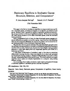
price captures all the informed consumers and half of the uninformed and sells 66 units. The higher price seller sells only to uninformed for a total of 6 units. If the two sellers tie on price, they each sell 36. One can see that the best response to a price of 100 is 99 and the best response to 99 is 98 and so on, down to a price of 10. But charging the maximum price of 100 guarantees you a profit of at least 600, while the highest profit available if one charges a price of 9 is 66 × 9 = 594, and so 9 is dominated by 100. A price of 100 also dominates all prices below 9. And so the best response to 10 is not 9 but 100. That is, there is a cycle of best responses like that in a RSP game and there is no pure strategy Nash equilibrium. Although this game is not a monocyclic game, numerical simulations suggest that the conclusion of Proposition 1 is still valid for this game: from most initial conditions orbits of the BR dynamics converge to a unique Shapley polygon that follows this best response cycle. However, what we can verify is that this class of games are positive definite and therefore, its mixed Nash equilibria are unstable under most known learning processes. This is analogous to the earlier result of Hopkins and Seymour (2002) on the instability of the original Varian model. Proposition 10 The discrete two player Varian model with strategy set of N prices {p1 , p2 , ..., pN } with U > 0 uninformed buyers and I > 0 informed buyers gives rise to a positive definite game. Thus, any mixed strategy equilibrium is unstable with respect to the BR dynamics. Proof: In the Appendix. Yet, curiously as MOS report, the data, aggregated across time and different subjects, seems remarkably close to that which would have been generated by Nash equilibrium play. Prices are somewhat higher, however. Furthermore, this distribution is stable across time and different experimental sessions. Given the result on instability above, this is not consistent with fictitious play with classical beliefs, under which the time average should diverge. The Nash and empirical distributions are illustrated in Figure 2.14 MOS also report that there is significant autocorrelation in prices, which is suggestive of price cycles produced by a learning process which has not converged. We have calculated the TASP for this game by numerical simulation of the BR dynamics and the resulting distribution is also given in Figure 2. It is clearly closer to the data than is the Nash equilibrium, though it is not an exact fit. The difference between the empirical distribution and the TASP can be ascribed to two possible explanations. First, under stochastic fictitious play, the time average of play will only approach the TASP asymptotically. The experimental data may be influenced by the initial conditions of the experiment. Second, under stochastic fictitious play, play will only approach the TASP as δ approaches 1 and β approaches infinity. Estimates of these parameters from other experiments (see, for example, Battalio et al. 14
Following MOS, the figure gives the cumulative distribution for the mixed strategy equilibrium of the original Varian model which assumes a continuum of prices. Mixed equilibria of the discrete game have distributions which are almost identical.
22
1
0.9
N 0.8
T
D
0.7
0.6
0.5
0.4
0.3
0.2
0.1
0
0
10
20
30
40
50
60
70
80
90
100
Price Figure 2: Cumulative distribution functions for prices in the Varian duopoly model under the mixed Nash equilibrium (N), the TASP (T) and the data from the experiments of Morgan et al. (2006) (D). (2001), Camerer and Ho (1999), Cheung and Friedman (1997) among others) are not close to these limiting values and this may explain what we see here. For example, a low value of δ would imply something closer to a simple best response or Edgeworth cycle, which in the current game implies undercutting on prices as far as 10 and then a return to 100. This in turn would imply a uniform distribution on [10, 100]. The actual empirical distribution is somewhere between the TASP distribution and such a uniform distribution. Distinguishing between these explanations would require a careful econometric investigation, which is beyond the scope of the current work. Obviously, there are other potential explanations for behaviour of subjects in this experiment. For example, a perturbed equilibrium such as a logit equilibrium could also exhibit a stochastically higher distribution of prices than in Nash equilibrium. However, while they might offer similar point predictions about the time average of play, there is a crucial difference between the TASP and such equilibrium concepts such as logit or quantal response equilibrium.
23
The TASP is produced by non-stationary cyclical play, in contrast to the stationary play implied by equilibrium whether it be Nash or perturbed Nash. Thus, the nonstationary behaviour of subjects (also reported in similar experiments by Cason and Friedman (2003), Cason, Friedman and Wagener (2005) and by Brown Kruse et al. (1994)) makes a static equilibrium concept difficult to apply to these circumstances. Stochastic fictitious play with classical beliefs would predict cyclic behaviour in Morgan et al.’s (2006) experiments as the equilibrium is unstable, but at the same time would predict the time average of play to be divergent. To our knowledge, only the current theory, that identifies stable cycles in a learning process, can simultaneously explain how the time average of data is similar but distinct from Nash, while at the same time the distribution of prices is non-stationary. To which it might be replied, play in experiments on games with mixed strategy equilibria is always non-stationary. Such a finding was first reported by Brown and Rosenthal (1990) but has been confirmed by many subsequent studies. Importantly, Brown and Rosenthal (1990) were looking at data on constant sum games in which mixed strategy equilibria are attractors under stochastic fictitious play (Hofbauer and Sandholm (2002), Hofbauer and Hopkins (2005)). Thus, under stochastic fictitious play under classical beliefs, asymptotically one would expect stationary equilibrium play. However, this is no longer true with recency, with stationary play only possible as one takes the limit of δ to one (see Proposition 9). Thus, the difference between stable and unstable equilibria under recency is much smaller than under classical beliefs. But what the TASP implies about play is more precise than it simply being nonstationary. Specifically, play should follow a best response cycle even as empirical frequencies converge. In the context of oligopoly games such as those studied by Brown Kruse et al. (1994), Cason and Friedman (2003), Morgan, Orzen, and Sefton (2006) and Cason, Friedman and Wagener (2005), this would imply prices progressively falling, followed by a relatively rapid rise to a high average price, followed by a slower fall and so on. But this is what Cason, Friedman and Wagener (2005) and Brown Kruse et al. (1994) both report. In contrast, if the mixed strategy equilibrium were stable under stochastic fictitious play, players’ mixed strategies for δ close to 1 should be close to Nash equilibrium frequencies. Play would not be stationary but there should not be the distinct cycles present in the unstable case. Thus, a clearer test of the TASP would be comparative. Run two apparently similar games such as A and B in (1) experimentally and test for differences in behaviour. This has been done by Engle-Warnick and Hopkins (2005). They investigate two 3 × 3 games that are asymmetric in the sense of Section 7, and each having a unique mixed strategy equilibrium. The equilibrium of one game is unstable and the other stable under classical fictitious play. The time average of play converges in both cases, rejecting the main predictions of the model under classical beliefs, while being consistent with weighted stochastic fictitious play. The level of serial dependence is higher, that is cycling is more pronounced, in the unstable game, which gives support to our current hypothesis. Clearly, however, if the differences were small or non-existent, it would be
24
strong evidence against the TASP.
8.2
When is the TASP distinct from Nash equilibrium?
We move on to our second goal: to identify games where the TASP is significantly different from Nash equilibrium. Note that for any game that is completely symmetric the mixed Nash equilibrium and the TASP will be identical. For example, if we take the general RSP game in (1) and set a1 = a2 = a3 > b1 = b2 = b3 , then the Nash equilibrium and the TASP are both equal to (1/3, 1/3, 1/3). Since both the TASP and the Nash equilibrium are continuous in payoffs, games that are almost symmetric will give rise to only small differences beween the TASP and Nash. The game B in (1) is an example of this. However, it is possible to construct examples where the differences are much larger. Take this variant of the RSP game. 0 -3 1 C = 1 0 -3 -3 b2 0
(24)
For b2 small, it can be verified that the game is positive definite and thus the mixed equilibrium is unstable. Note that if we take the limit of b2 to zero, the Nash equilibrium approaches (9, 13, 12)/34 ≈ (0.26,0.38,0.35), still close to the centre of the simplex. In contrast, the limit of the TASP as b2 goes to zero is (0,1,0). The high weight placed on the second strategy is a consequence of the vertex A2 of the Shapley polygon approaching the point (0,1,0) as b2 approaches zero. On the edge between A1 and A2 , the BR dynamics are x˙ 2 = 1 − x2 and so when x2 is close to one, the speed at which they approach A2 is extremely slow. Thus, a very long time is spent on the second edge. In the following game the difference between the TASP and any Nash equilibrium is even more striking. It consists of a RSP game with the addition of another strategy D (for “Dumb” as for c > 0 it is not a best response to any pure strategy). 0 -3 1 c 1 0 -3 c RSP D = -3 1 0 c d d d 0
(25)
When c > 0, then this game has no pure strategy equilibrium. For example if c = 1/10 and d = −1/10, the unique Nash equilibrium is fully mixed and equal to (1, 1, 1, 17)/20. It is possible to calculate that, under the BR dynamics, the Nash equilibrium is a saddle with the stable manifold being the line satisfying x1 = x2 = x3 . Thus for almost all initial conditions, the BR dynamics diverge. When the weights on the first three strategies are no longer equal, the fourth strategy is not a best reply, so that any weight on x4 tends to die out as play diverges from equilibrium. But on the face where x4 = 0, 25
we have the original RSP game, and with the above parameter values, there will be a Shapley polygon on the face. Indeed, it is easy to calculate the TASP in this case as (1/3, 1/3, 1/3, 0). That is, the Nash equilibrium places a weight of 17/20 on the fourth strategy and the TASP places no weight on it whatsoever. For this game, the Nash equilibrium and the TASP are quite distinct. A potential difficulty in testing the above examples experimentally is that the clarity of the above predictions is reduced once noise is introduced. For example, the time average of any limit cycle of the PBR dynamics in the game RSPD will give positive weight to the strategy D, as the PBR dynamics always give positive weight to all strategies. Similarly, also in RSPD, the logit equilibrium corresponding to the Nash equilibrium will place greater weight on R, S and P than the Nash equilibrium does. Nonetheless, the initial distinctions are so great, we would expect some difference to remain. Thus, if play was closer to Nash equilibrium than to the TASP even when monetary incentives were high, we could reject the TASP in favour of Nash equilibrium. We make this point to emphasise that the current theory does offer testable predictions. Furthermore, the comparative statics will be different. Suppose we double all the payoffs in the matrix (25). The Nash equilibrium will not change. However, as such a change is similar to an increase in the parameter β, the logit equilibrium will move closer to the Nash equilibrium, and the weight it places on strategy D will increase. But an increase in payoffs will mean that stochastic fictitious play should approach the TASP more closely. That is, the weight on D should decrease, a change that is in the opposite direction to that of the logit equilibrium.
8.3
Are the Comparative Statics of the TASP Different from those of Nash Equilibrium?
As point predictions are sometimes difficult to test, we can also perform some simple comparative statics. Take a symmetric RSP game and then add a constant to the payoffs to the first strategy. ε −a + ε b + ε b 0 −a (26) −a b 0 If the parameter ε is zero, the game is entirely symmetric and the Nash equilibrium and the TASP are equal to (1/3, 1/3, 1/3). We can calculate the weight placed on the first strategy in the Nash equilibrium as 1 b−a +ε 2 3 3(a + ab + b2 ) That is, when a > b, which would imply that the mixed equilibrium is unstable under the BR dynamics, we have a counterintuitive result: an increase in the payoffs of the first strategy results in a reduction in the frequency of the first strategy in the mixed 26
equilibrium. In contrast, one can calculate that ¯ ∂ x˜1 ¯¯ (a − b)2 (a + b) = ∂ε ¯ε=0 3ab(a2 + ab + b2 ) log(a/b)
Thus, the effect is the opposite. When a > b, so that the TASP exists, an increase in the payoff to the first strategy results in a greater weight on the first strategy in the TASP.
8.4
Does the TASP Give a Prediction Distinct from that of Other Learning Models?
Fictitious play is not the only model of learning in games. It is important to clarify whether the prediction of convergence to the TASP is robust across different models, or whether other models suggest a completely different outcome. First, reinforcement learning in economics has been popularised by Erev and Roth (1998). Hopkins (2002) shows that the asymptotic predictions of their model are largely similar to those of fictitious play. For example, mixed equilibria in asymmetric games are generically unstable under reinforcement learning. Now, the basic one parameter model of Erev and Roth has a step size that is of order 1/t so that its time average will not converge to a mixed equilibrium in such circumstances. However, their three parameter model (which allows for noise and recency) will, like weighted stochastic fictitious play, be ergodic (Hopkins (1999c)) and therefore will have a convergent time average even when all equilibria are unstable. Whether this time average is related to the TASP is, however, at this point pure speculation. Second, there are learning models that have better convergence properties than fictitious play (see Young (2004) for a recent survey). One is due to Hart and MasColell (2000). In their model, the time average of play converges to the set of correlated equilibria of the game in question. In the RSP games the only correlated equilibrium is the Nash equilibrium (see Viossat (2005)) and so the Hart—Mas-Colell model predicts learning should always converge in this class of games, something that is in distinct contrast with the learning models considered here. In contrast, the Shapley game (Example 5 in this paper) is an example of a game where if beliefs cycle on the Shapley polygon, play follows the best response cycle that avoids the outcomes where both players receive a payoff of zero. This pattern of play is a correlated equilibrium. In such games the model of Hart and Mas Colell is not necessarily in conflict with the weighted version of stochastic fictitious play. However, the set of correlated equilibria is typically large, whereas the TASP is a single point, and as a prediction it offers greater precision. Finally, Foster and Young (2003) introduce a learning model where each player forms hypotheses about the strategies of her opponents and plays (almost always) a best response given her beliefs. When her observations of her opponents’ play are sufficient to reject her current hypothesis, she forms a new hypothesis. Foster and Young show that this learning model always converges to Nash equilibrium. More precisely, there are 27
parameter values of the model, such that players’ mixed strategies will be close to some Nash equilibrium for most of the time in any game. It thus offers a different prediction from stochastic fictitious play, whether beliefs are weighted or classical, which predicts that players’ mixed strategies should diverge from equilibrium in some games such as game B in (1).
9
Conclusions
Much of the recent work on learning in games has been concerned with selection between different Nash equilibria, or with providing an adaptive basis for equilibrium play. In this paper, we take a completely different approach. We found that in some games learning under stochastic fictitious play has a non-equilibrium outcome, which nevertheless gives a precise prediction about play. We introduced the TASP (time average of the Shapley polygon), building on earlier results by Shapley (1964) and Gaunersdorfer and Hofbauer (1995), as an outcome for the time average of play. This we suggest could be useful in understanding behaviour in a number of economically interesting models, including the Varian (1980) model of price dispersion and Bertrand-Edgeworth competition. This also represents one of the few attempts at analysis of learning in games when players place greater weight on more recent experience. Most previous work on stochastic fictitious play and reinforcement learning has examined models with learning that slows over time. This is despite the fact that most empirical work fitting learning models to experimental data has found that weighting recent experience more highly gives a better fit. The two types of models do give similar predictions when considering games that have Nash equilibria that are stable under learning. The finding here, however, is that they give radically different results when considering equilibria that are unstable. In this paper, we have obtained a series of theoretical results on learning. These are asymptotic results that also depend on taking limiting values of two key parameters that determine the level of optimisation and recency respectively. This may generate some skepticism about their empirical relevance, firstly because real phenomena occur in finite time, and second, because estimates of these parameters from experimental data are not close to these limit values. However, if the TASP is to be dismissed on this basis, so should Nash equilibrium. If one takes stochastic fictitious play or its variants such as EWA learning (Camerer and Ho (1999)) seriously as models of human behaviour, Nash equilibrium play only occurs as the asymptotic limit of learning behaviour, and then only if the appropriate parameters are at their limit values. Indeed, recent research has found that perturbed equilibria such as quantal response equilibria (McKelvey and Palfrey (1995); Anderson et al. (2002)), that allow the optimisation parameter not to be at its limit, often fit experimental data better. The point is that the TASP, like Nash equilibrium, offers a qualitative prediction about behaviour in games that can be made without any parameter estimation. Thus, 28
these concepts can still be empirically useful as an initial hypothesis. One can then go on to make their predictions more precise by using richer models that employ more parameters. In the case of the TASP, it can be generalised by looking at the time average of stochastic fictitious play for which there are two parameters than can affect the long run outcome. Just as for quantal response equilibria, there is an optimisation parameter, but in weighted stochastic fictitious play there is also the parameter that controls the degree of forgetting or recency. However, these parameters have been jointly estimated in existing attempts to fit stochastic fictitious play to experimental data (see Cheung and Friedman (1997), Camerer and Ho (1999), Battalio et al. (2001) among others). There is, therefore, no fundamental barrier to taking the TASP to the data.
Appendix Proof of Proposition 1: Let B i be set of points x ∈ S N with i being the unique best reply, and B ij be set of points x ∈ S N with precisely two pure best replies i and j. The i union of all and has full (N −1) dimensional Lebesgue measure in S N . SnB isi open, Sn dense Let B = i=1 B ∪ i=1 B i−1,i . We will show that B is strongly forward invariant under the best response dynamics and all orbits there approach a unique Shapley polygon contained in B. Suppose x ∈ B 1 , i.e., (Ax)1 > (Ax)j for all j 6= 1. Then x(t) = e−t x + (1 − e−t )e1 and (Ax(t))1 = e−t (Ax)1 and for j 6= 1, 2, (Ax(t))j = e−t (Ax)j + (1 − e−t )aj1 < e−t (Ax)j < e−t (Ax)1 = (Ax(t))1 .
(27)
So along the ray from x to e1 , the best response can only switch from 1 to 2 which indeed must happen for some t > 0, since a21 > 0. Hence the orbit hits B 12 . The only way to continue is towards e2 . Repeating the above argument shows that orbits in B 12 move into B 23 , etc, and finally from B N 1 back into B 12 . This defines a continuous return map f : B N1 → B N1 . f is single-valued as solutions starting in B are unique. f is a composition of projective maps and hence a projective map itself. Being uniformly continuous, it can be extended to the closure ¯ N1 of the convex polyhedron B N1 . A fixed point of f in B N1 generates a closed B orbit under the best response dynamics, an invariant N-gon, i.e., a Shapley polygon. ¯ N1 contains the interior equilibrium x∗ we cannot directly apply a fixed However, since B point theorem to prove the existence of the Shapley polygon. Define V (x) = maxi (Ax)i . As shown above for x ∈ B 1 , along any solution x(t) ∈ B, V (x(t)) = e−t V (x). Hence V (x(t)) → 0, as t → ∞. The set B0 = B ∩ {x ∈ S N : V (x) = 0} is forward invariant and its closure contains xβ < 0 holds for each equilibrium xˆβ (by assumption no equilibrium, since V (ˆ xβ ) = xˆβ·Aˆ ∗ for the interior equilibrium x , and automatically for each boundary equilibrium of a monocyclic game). Since V (x∗ ) < 0 and V (ei ) = ai+1,i > 0, each ray from x∗ to a 29
point x near ei hits the set {V = 0} in a unique point which is thus contained in B0i+1 = B i+1 ∩ {x ∈ S N : (Ax)i+1 = 0}, a convex (N − 2)—dimensional set. The ¯0N1 is a closed and convex sets B0i,i+1 are therefore (N − 3)—dimensional. The closure B polyhedron, mapped by f into itself. So by Brouwer’s fixed point theorem, it contains a fixed point (which cannot be an equilibrium). Its orbit is a Shapley polygon Γ. To prove uniqueness and stability of this Shapley polygon, we use the projective metric d, as in Gaunersdorfer and Hofbauer (1995). The distance between two points x, y ∈ int B0N1 (the relative interior15 of B0N1 ) is given by the logarithm of the double ratio µ ¶ xp yp d(x, y) = | log : | xq yq with p, q being the intersection points of the line through x, y with the relative boundary ¯0N1 ) ⊆ B ¯0N1 , we have d(f (x), f (y)) ≤ d(x, y) for x, y ∈ int B0N 1 . Now of B0N1 . Since f (B (27) holds for j 6= 1, 2 with a strict inequality even under the weaker assumption (Ax)1 ≥ (Ax)j for all j and (Ax)1 > (Ax)2 . This shows that for x ∈ bd B0N1 (with at least a third best reply j besides N and 1), f (x) ∈ int B0N1 = B0N1 ∩ int S N . Hence ¯0N1 ) ⊆ int B0N1 , and hence d(f (x), f (y)) < d(x, y) for x, y ∈ int B0N1 with x 6= y. f (B Hence, by a variant of Banach’s fixed point theorem, the fixed point of f is unique and ¯0N1 . attracts all orbits in B Hence all orbits in B approach the Shapley polygon Γ, and Γ is Lyapunov stable. Remark. The complement of B consists of all points with at least two non— successive pure best replies (or more than two best replies). The behavior of orbits starting outside B depends in an intricate way on the payoff matrix. Typically, solutions starting in x ∈ / B are not unique. From every x ∈ / B (except possibly x∗ ) there exists at least one solution that enters B and hence converges to Γ. The solutions staying in S N \ B can converge to a Nash equilibrium or, for N ≥ 5, to an unstable Shapley polygon contained in S N \ B. Proof of Proposition 2: We first show that a positive definite game has only finitely many equilibria. Suppose there are two equilibria, xˆ and x˜, satisfying (Aˆ x)1 = (Aˆ x)2 = · · · = (Aˆ x)N
(28)
and similar for x˜. Then (ˆ x − x˜)·A(ˆ x − x˜) = 0 contradicts positive definiteness. Applying these to ‘subgames’ (with restricted support) which are still positive definite we see that each face of SN contains at most one equilibrium. In particular, this implies that every solution of the BR dynamics is piecewise linear, see Hofbauer (1995). We now use the Ljapunov function from Hofbauer (2000) V (x) = max(Ax)i − x·Ax. i
15
(29)
The relative interior int C of a convex set C ⊆ RN is the interior of C within the affine space spanned by it. The relative boundary of C is then given by bd C = C¯ \ int C.
30
Note that V (x) ≥ 0 for all x and V (x) = 0 if and only if x is a NE. We show that in a positive definite game, V (x(t)) increases along almost all solutions x(t) of the BR dynamics starting near an equilibrium xˆ. Since V (x) = (b − x)·Ax for b ∈ b(x), we have along a piecewise linear solution V˙ = b·Ax˙ − x·Ax ˙ − x·Ax˙ = (b − x)·A(b − x) − x·Ax ˙ = (b − x)·A(b − x) − V (x) (30) The first term is nonnegative in a positive definite game. Suppose that xˆ is an equilibrium with (28). (Usually such equilibria are completely mixed.) Let I be the support of xˆ. Suppose for some x 6= xˆ, I ⊆ b(x). Then xˆ ∈ b(x) and xˆ·Ax ≥ x·Ax. On the other hand, (28) implies xˆ·Aˆ x = x·Aˆ x. Hence (ˆ x −x)·A(ˆ x −x) ≤ 0, contradicting positive definiteness. Hence, for all x 6= xˆ, b(x) does not contain I. So b(x) is contained in boundary faces opposite to xˆ. Therefore the distance |b − x| (with b ∈ b(x)) has a positive lower bound for x close to (but different from) xˆ. Using positive definiteness again, this shows that the first term, (b−x)·A(b−x), in the RHS of (30) has a positive lower bound, so V increases along each orbit near xˆ. Hence xˆ is a repellor. Finally consider an arbitrary equilibrium xˆ with I denoting its set of pure best replies. Then for x close to xˆ, the pure best replies to x are contained in I. Hence the face spanned by I is locally (near xˆ) invariant under the BR dynamics (and attracts orbits nearby). Hence we can apply the above argument to the game with restricted strategy set I and conclude that all orbits in this face starting close to xˆ move away from xˆ. Hence xˆ is unstable. This argument works whenever I has at least two elements, i.e. xˆ is not a strict equilibrium. Proof of Proposition 3:16 We take the Liapunov function from Hofbauer (2000) and Hofbauer and Sandholm (2002) U (x) = π(p(x), x) − π(x, x) = (p(x) − x) · Ax + λ(v(p(x)) − v(x)) ≥ 0
(31)
where again λ = β −1 . Then U has a minimum on S N at xˆβ . Then, under the dynamics (14), we have U˙ = (p(x) − x) · A(p(x) − x) + λ(p(x) − x) · (v0 (p(x)) − v0 (x)) Now, the second term on the right hand side is negative by the concavity of v(·), but the first term of right hand side is positive as A is positive definite by assumption. Then in the neighbourhood of x∗ , for β sufficiently large, we have U˙ positive, and the perturbed equilibrium is a repellor. Proof of Proposition 4: The Shapley polygon Γ with corners A1 , · · · , AN is an attractor (= asymptotically invariant set) for (3) whose basin of attraction B is open and dense in S N , and the complement S N \ B has zero Lebesgue measure. For small γ > 0, the map (2) has an attractor nearby with basin of attraction exhausting B as 16
This result on instability is proved by means of a Liapunov function, but one could also apply the local linearisation result of Hopkins (1999b).
31
γ → 0. (This is well-known for discretisations of differential equations, see e.g. Stuart and Humphries (1996) or Garay and Hofbauer (1997). The corresponding result for differential inclusions needed here for the BR dynamics follows readily by combining their results and methods of proof with those in Benaïm et al. (2005)). The time average w ˆt converges to a space average over the attractor of the map (2) with respect to some invariant measure, which tends to the unique measure invariant under the BR dynamics concentrated on the Shapley polygon in the limit as γ goes to zero (Miller and Akin (1999)). The space average with respect to this unique invariant measure equals the time average given by the expression (5). The other limit follows from the relation 1X 11 (xt+1 − x1 ) → 0, (b(xs ) − xs ) = t s=1 tγ t
wt − w ˆt = as t approaches infinity.
Proof of Proposition 6: If the player chooses action i then denote that event as i and event operator fi . Norman (1968) defines a Markov process on a metric space with metric d to be “strictly distance diminishing” if ρ(fi ) < 1 for all i where ρ(f ) = sup x6=x0
d(f (x), f (x0 )) . d(x, x0 )
Lemma 1 The Markov process defined by stochastic fictitious play with forgetting, that is, with belief updating rule (12) with γ t = 1 − δ is strictly distance diminishing with respect to the standard Euclidean metric. Proof: Given arbitrary states x, x0 , fi (x) = (1 − δ)Xi + δx and fi (x0 ) = (1 − δ)Xi + δx0 . It is easy to show therefore that d(fi (x), fi (x0 )) = δd(x, x0 ) and ρ(fi ) = δ for all possible events. Let Tn (x) be the set of states reached with positive probability in n steps if we start at x. Let d(S1 , S2 ) be distance between two subsets S1 and S2 of the state space. That is, d(S1 , S2 ) = inf0 d(x, x0 ) x∈S1 ,x ∈S2
Then Norman (1968) was able to show that if the following condition holds lim d(Tt (x), Tt (x0 )) = 0 for all x, x0 ∈ S
t→∞
(32)
then a strictly distance diminishing Markov process is ergodic. Norman’s result (Theorem 2.2, p66) applies to strictly distance diminishing Markov processes on a compact metric space, here S N , where the number of possible events are finite, here N. So, we simply need to verify the condition (32). From an arbitrary initial state x1 there is a positive probability that each player chosen continues to choose the first action for an indefinite number of periods. As this run of play continues, xt will approach the state 32
X1 . This state is therefore accessible from any initial state and from the theorem of Norman, the Markov process is ergodic. Proof of Proposition 7: The probability measure ν 1,β is an invariant measure of the dynamics induced by φβ . Hence by the Poincaré recurrence theorem, its support is contained in the Birkhoff center of φβ (see e.g. Benaïm, 1998, Corollary 3.2). The second assertion follows from Theorem 3.2 of Fort and Pagès (1999). According to this theorem, it suffices to verify that properties (I) and (II) below hold in order to conclude that ν 1,β (ˆ xβ ) = 0. (I) The process (xt ) can be written as xt+1 − xt = γH(xt , ω t+1 )
(33)
where (ωt ) is a sequence of i.i.d. random variables, and (x, ω) 7→ H(x, ω) is a bounded measurable function continuous in x at point xˆβ , for almost every ω. (II) (a) There exists a C 2 real valued function U defined on a neighborhood W of xˆβ in S N such that for all x ∈ W \ {ˆ xβ }, h∇U (x), φβ (x)i > 0 and U (x) > U(ˆ xβ ) xβ )⊥ such that the variance term (b) there exists u ∈ ker D2 U (ˆ
X xt+1 − xt E(h , ui2 |xt = xˆβ ) = h−ˆ xβ + ei , ui2 xˆβ,i γ i=1 N
is positive.
Let (ωt ) be a sequence of independent uniformly distributed random variables in [0, 1]. P Pi Set H(x, ω) = −x + ei for i−1 p (x) ≤ ω < p (x) and i = 1, . . . , N. Then j=0 j j=0 j Pi−1 N x 7→ H(x, ω) is continuous at xˆβ for every ω ∈ [0, 1] \ ∪i=1 { j=0 xˆβ,j }, by continuity of the map x 7→ p(x). Furthermore Pr(H(x, ωt ) = −x + ei ) = pi (x). Hence, we can always assume that (xt ) satisfies (33). We now check (II). The function U(x) = π(p(x), x) introduced in the proof of proposition 2 satisfies (a). A simple computation yields
and, using λ = β −1 ,
∇U(x) = AT (p(x) − x) − Ax − λv 0 (x)
D2 U(x) = AT p0 (x) − (A + AT ) − λv 00 (x) = −βAT v 00 (p(x))−1 A − (A + AT ) − v 00 (x)/β
so that for β large enough D2 U (x) is invertible ( β1 det(D2 U(x)) 7→ − det(A∗ v00 (p(x))−1 A) 6= 0) and condition (b) reduces to prove that N X h−ˆ xβ + ei , ui2 xˆβ,i > 0 i=1
33
for some u in the tangent space of S N . This is obviously true since the family (ei − xˆβ )i=1,...,N spans the tangent space of S N . Proof of Proposition 10: With prices {p1 , p2 , ..., pN } (given in ascending order), the payoff matrix has the form p1 (U + I)/2 p1 (U/2 + I) . . . p1 (U/2 + I) p2 U/2 p2 (U + I)/2 . . . p2 (U/2 + I) A= .. .. .. ... . . . pN U/2 . . . pN (U + I)/2 pN U/2
where U is the number of uninformed and I is the number of informed.
Let A0 be the N −1×N −1 matrix formed by the formula a0,ij = aij −aiN −aN j +aNN . The matrix A is positive definite with respect to RN 0 if A0 is positive definite. We find that pN − p1 pN − p2 pN − p3 . . . pN − pN−1 pN − p2 pN − p2 pN − p3 . . . pN − pN−1 .. pN − p3 pN − p3 . . . . A0 + AT0 = I pN − p3 .. .. .. .. ... . . . . ... . . . pN − pN−1 pN − pN −1 pN − pN−1
One can subtract columns of a matrix from other columns without any change to its determinant. Here, we can can subtract the N − 1th column from all others, then the (N − 2)th from all to its left and continue recursively until we have an upper triangular matrix with p2 − p1 , p3 − p2 , ...., pN − pN−1 on its diagonal. The determinant is clearly positive. One can repeat the procedure for each principal minor and obtain a similar result. Thus, A0 is positive definite, and hence so is A with respect to RN 0 . Instability of mixed strategy equilibria then follows from Proposition 2.
References Anderson, S., J. Goeree, and C. Holt (2002),“The logit equilibrium: a perspec˝ tive on intuitive behavioral anomalies,” Southern Economic Journal, 69, 21U47. Battalio, R., L. Samuelson, and J. Van Huyck (2001). “Optimization Incentives And Coordination Failure In Laboratory Stag Hunt Games,” Econometrica, 69, 749-764. Benaïm, M. (1998). “Recursive algorithms, urn processes and chaining number of chain recurrent sets,” Ergodic Theory and Dynamical Systems, 18, 53-87. Benaïm, M. (1999). “Dynamics of stochastic algorithms,” in Séminaire de Probabilités XXXIII, J. Azéma et al. Eds, Berlin: Springer-Verlag.
34
Benaïm, M., Hirsch, M.W. (1999). “Mixed equilibria and dynamical systems arising from fictitious play in perturbed games,” Games and Economic Behavior, 29, 36-72. Benaïm, M., J. Hofbauer, and S. Sorin (2005). “Stochastic approximation and ˝ differential inclusions,” SIAM Journal of Control and Optimization, 44, 328U348. Benaïm, M., J. Weibull (2003). “Deterministic approximation of stochastic evolution in games”, Econometrica, 71, 873-903. Benveniste, A., M. Métivier, and P. Priouret (1990). Adaptive Algorithms and Stochastic Approximations. Berlin: Springer-Verlag. Berger, U. (1995). Replikator- und Best Response Dynamik für 3 × 3 Bimatrixspiele. Master’s thesis. University of Vienna. Brown, J., Rosenthal, R. (1990). “Testing the minimax hypothesis: a reexamination of O’Neill’s game experiment,” Econometrica, 58, 1065-1081. Brown Kruse, J., S. Rassenti, S.S. Reynolds and V.L. Smith (1994). “BertrandEdgeworth Competition in Experimental Markets,” Econometrica, 62, 343-371. Burdett, K., Judd, K. (1983). “Equilibrium price dispersion,” Econometrica, 51, 955-969. Camerer, C., Ho, T-H. (1999). “Experience-weighted attraction learning in normal form games,” Econometrica, 67, 827-874. Cason, T., Friedman, D. (2003). “Buyer search and price dispersion: a laboratory study,” Journal of Economic Theory, 112, 232-260. Cason, T., Friedman, D., and Wagener F. (2005). “The Dynamics of Price Dispersion or Edgeworth Variations,” Journal of Economic Dynamics and Control, 29, 801-822. Cheung, Y-W., Friedman, D. (1997). “Individual learning in normal form games: some laboratory results,” Games and Economic Behavior, 19, 46-76. Cowan, S. (1992). “Dynamical Systems arising from Game Theory”, Ph.D. thesis, University of California at Berkeley. Edgeworth, F. Y. (1925), “The Pure Theory of Monopoly,” in Papers Relating to Political Economy, vol. 1, New York: Burt Franklin. Ellison, G., Fudenberg, D. (2000). “Learning purified mixed equilibria,” Journal of Economic Theory, 90, 84-115. Engle-Warnick, J., Hopkins, E. (2005). “A simple test of learning theory,” working paper. 35
Erev, I., Roth, A.E. (1998). “Predicting how people play games: reinforcement learning in experimental games with unique, mixed strategy equilibria,” American Economic Review, 88, 848-881. Fort, J-C., Pagès, G. (1999). “Asymptotic behavior of a Markovian stochastic algorithm with constant step,” SIAM Journal of Control and Optimization, 37, 1456-1482. Foster, D.P., Young, H.P. (2003). “Learning, hypothesis testing, and Nash equilibrium,” Games and Economic Behavior, 45, 73-96. Fudenberg, D., Kreps D. (1993). “Learning mixed equilibria,” Games and Economic Behavior, 5, 320-367. Fudenberg, D., Levine, D. (1998). The Theory of Learning in Games. Cambridge, MA: MIT Press. Garay, B., Hofbauer J. (1997). “Chain recurrence and discretization,” Bull. Austral. Math. Soc. , 55, 63-71. Gaunersdorfer, A., and J. Hofbauer (1995). “Fictitious play, Shapley Polygons, and the Replicator Equation,” Games and Economic Behavior, 11, 279-303. Gilboa, I., Matsui, A. (1991). “Social stability and equilibrium,” Econometrica, 59, 859-867. Hart, S., Mas-Colell A. (2000). “A simple adaptive procedure leading to correlated equilibrium,” Econometrica, 68, 1127-1150. Hofbauer, J. (1995). “Stability for the best response dynamics,” working paper, University of Vienna. Hofbauer, J. (2000). “From Nash and Brown to Maynard Smith: equilibria, dynamics and ESS,” Selection, 1, 81-88. Hofbauer, J., Hopkins, E. (2005). “Learning in Perturbed Asymmetric Games”, Games and Economic Behavior, 52, 133-152. Hofbauer, J., Sandholm, W.H. (2002). “On the global convergence of stochastic fictitious play”, Econometrica, 70, 2265-2294. Hofbauer, J., Sandholm, W.H. (2005). “Evolution in Games with Randomly Disturbed Payoffs”, forthcoming Journal of Economic Theory. Hofbauer, J., Sigmund, K. (1998). Evolutionary Games and Population Dynamics. Cambridge, UK: Cambridge University Press. Hopkins, E. (1999a). “Learning, matching and aggregation,” Games Econ. Behav., 26, 79-110. 36
Hopkins, E. (1999b). “A note on best response dynamics,” Games Econ. Behav., 29, 138-150. Hopkins, E. (1999c). “Two Competing Models of How People Learn in Games,” working paper version, University of Edinburgh. Hopkins, E. (2002). “Two Competing Models of How People Learn in Games,” Econometrica, 70, 2141-2166. Hopkins, E., Seymour, R. (2002). “The Stability of Price Dispersion under Seller and Consumer Learning”, International Economic Review, 43, 1157-1190. Krishna, V., Sjöström, T. (1998). “On the convergence of fictitious play”, Mathematics of Operations Research, 23, 479-511. McKelvey, R.D., Palfrey, T.R. (1995). “Quantal response equilibria for normal form games,” Games and Economic Behavior, 10, 6-38. Miller, W., Akin, E. (1999). “Invariant measures for set-valued dynamical systems”, Transactions of the American Mathematical Society, 351, 1203-1225. Monderer, D., Shapley, L.S. (1996). “Fictitious Play Property for Games with Identical Interests”, Journal of Economic Theory, 68, 258-265. Morgan, J., H. Orzen, and M. Sefton (2006). “An Experimental Study of Price Dispersion”, Games and Economic Behavior, 54, 134-158. Norman, M.F. (1968). “Some convergence theorems for stochastic learning models with distance diminishing operators”, J. Math. Psych., 5, 61-101. Rosenmüller, J. (1971). “Über Periodizitätseigenschaften spieltheoretischer Lernprozesse”, Zeitschrift für Wahrscheinlichkeitstheorie und Verwandte Gebiete, 17, 259-308. Shapley, L. (1964). “Some topics in two person games,” in eds. M. Dresher et al., Advances in Game Theory. Princeton: Princeton University Press. Stuart, A.M., Humphries, A.R. (1996). Dynamical Systems and Numerical Analysis, Cambridge: Cambridge University Press. Tang, Fang-Fang (2001). “Anticipatory learning in two-person games: some experimental results”, Journal of Economic Behavior and Organization, 44, 221-232. Varian, H.R. (1980). “A model of sales,” American Economic Review, 70, 651-659. Viossat, Y. (2005). “Replicator Dynamics and Correlated Equilibrium: Elimination of All Strategies in the Support of Correlated Equilibria.” Working paper, École Polytechnique Paris. Young H.P. (2004): Strategic Learning and its Limits, Oxford University Press.
37