Lecture notes on Kinematics

Lecture notes on Kinematics Dr. Ing. Zdena Sant

CONTENTS 1

INTRODUCTION.....................................................................................................4

2

KINEMATICS OF A PARTICLE..............................................................................9

2.1

Velocity....................................................................................................................... 10

2.2 Acceleration ............................................................................................................... 11 2.2.1 Classification of motion ....................................................................................... 12 2.3 Orthogonal transformation ....................................................................................... 14 2.3.1 Orthogonal Transformation of Vector Quantities.................................................. 14 2.3.2 Velocity in matrix form using the orthogonal transformation................................ 16 2.3.3 Acceleration in matrix form using the orthogonal transformation ......................... 16 particle in Cylindrical coordinate system - r , ϕ , z .................................................... 17 2.4.1 The position vector .................................................................................................. 17 2.4.2 The velocity ......................................................................................................... 17 2.4.3 The acceleration................................................................................................... 18 2.4.4 Special cases............................................................................................................ 18

2.4

2.5 Particle trajectory...................................................................................................... 19 2.5.1 Rectilinear motion................................................................................................ 19 2.5.2 Curvilinear motion................................................................................................... 20 2.6 Harmonic motion ....................................................................................................... 20 2.6.1 Composition of harmonic motions in the same direction ...................................... 22 2.6.2 Composition of two perpendicular harmonic motions........................................... 23 2.7 3

Motion of a set of particles ........................................................................................ 23 SOLID BODY MOTION......................................................................................... 24

3.1 Translation motion of a solid body........................................................................... 24 3.1.1 Investigating kinematic quantities ........................................................................ 24 3.2 Rotation of a solid body around fixed axis................................................................ 25 3.2.1 Finding the velocity of an arbitrary point.............................................................. 26 3.2.2 Finding the acceleration of an arbitrary point B.................................................... 27 3.2.3 Solid body kinematics consequences (the geometrical dependency) ..................... 29 3.3

Universal planar motion............................................................................................ 31 3.3.1 The position............................................................................................................ 31

2 Dr. Ing. Zdenka Sant 10/2009

3.3.2 3.3.3

The velocity ......................................................................................................... 32 The pole of motion............................................................................................... 33 3.3.4 Finding the acceleration ........................................................................................... 35 3.3.5 The instantenous centre of acceleration – the pole of acceleration........................ 37 3.4

centre of the trajectory curvature ............................................................................. 38

3.5 Combined motion ...................................................................................................... 41 3.5.1 Kinematical quantities by means of combined motion.......................................... 42 3.5.2 The velocity ......................................................................................................... 42 3.5.3 The acceleration................................................................................................... 42 3.5.4 Coriolis acceleration ............................................................................................ 43 3.5.5 Finding the pole of motion by means of combined motion ................................... 44 3.6

Spherical motion of a Body ....................................................................................... 45

3.7

universal Space Motion Of a body ........................................................................... 47

4

SYSTEM OF BODIES........................................................................................... 48

4.1

Simultaneous rotations around concurrent axes ...................................................... 48

4.2

Simultaneous rotations around parallel axes............................................................ 49


1

INTRODUCTION

Design and analysis are two vital tasks in engineering. Design process means the synthesis during the proposal phase the size, shape, material properties and arrangements of the parts are prescribed in order to fulfil the required task. Analysis is a technique or rather set of tools allowing critical evaluation of existing or proposed design in order to judge its suitability for the task. Thus synthesis is a goal that can be reached via analysis. Mechanical engineer deals with many different tasks that are in conjunction to diverse working processes referred to as a technological process. Technological processes involve transportation of material, generation and transformation of energy, transportation of information. All these processes require mechanical motion, which is carried out by machines. To be able to create appropriate design of machine and mechanism the investigation of relation between the geometry and motion of the parts of a machine/mechanism and the forces that cause the motion has to be carried out. Thus the mechanics as a science is involved in the design process. Mechanics represents the science that includes Statics, Dynamics, and Mechanics of Materials. Statics provides analysis of stationary systems while Dynamics deals with systems that change with time and as Euler suggested the investigation of motion of a rigid body may be separated into two parts, the geometrical part and the mechanical part. Within the geometrical part Kinematics the transference of the body from one position to the other is investigated without respect to the causes of the motion. The change is represented by analytical formulae. Thus Kinematics is a study of motion apart from the forces producing the motion that is described by position, displacement, rotation, speed, velocity, and acceleration. In Kinematics we assume that all bodies under the investigation are rigid bodies thus their deformation is negligible, and does not play important role, and the only change that is considered in this case is the change in the position. Terminology that we use has a precise meaning as all the words we use to express ourselves while communicating with each other. To make sure that we do understand the meaning we have a thesaurus/glossary available. It is useful to clarify certain terms especially in areas where the terminology is not very clear. Structure represents the combination of rigid bodies connected together by joints with intention to be rigid. Therefore the structure does not do work or transforms the motion. Structure can be moved from place to place but it does not have an internal mobility (no relative motion between its members). Machines & Mechanisms – their purpose is to utilize relative internal motion in transmitting power or transforming motion. Machine – device used to alter, transmit, and direct forces to accomplish a specific objective. Mechanism – the mechanical portion of a machine that has the function of transferring motion and forces from power source to an output. Mechanism transmits motion from drive or input link to the follower or the output link. 4 Dr. Ing. Zdenka Sant 10/2009

Planar mechanism – each particle of the mechanism draws plane curves in space and all curves lie in parallel planes. The motion is limited to two-dimensional space and behaviour of all particles can be observed in true size and shape from a single direction. Therefore all motions can be interpreted graphically. Most mechanisms today are planar mechanism so we focus on them. Spherical mechanism – each link has a stationary point as the linkage moves and the stationary points of all links lie at a common location. Thus each point draws a curve on the spherical surface and all spherical surfaces are concentric. Spatial mechanism – has no restriction on the relative motion of the particles. Each mechanism containing kinematical screw pair is a spatial mechanism because the relative motion of the screw pair is helical. The mechanism usually consists of: Frame – typically a part that exhibits no motion Links – the individual parts of the mechanism creating the rigid connection between two or more elements of different kinematic pair. (Springs cannot be considered as links since they are elastic.) Kinematic pair (KP) represents the joint between links that controls the relative motion by means of mating surface thus some motions are restricted while others are allowed. The number of allowed motions is described via mobility of the KP. The mating surfaces are assumed to have a perfect geometry and between mating surfaces there is no clearance. Joint – movable connection between links called as well kinematic pair (pin, sliding joint, cam joint) that imposes constrains on the motion Kinematic chain is formed from several links movably connected together by joints. The kinematic chain can be closed or opened according to organization of the connected links. Simple link – a rigid body that contains only two joints Complex link – a rigid body that contains more than two joints Actuator – is the component that drives the mechanism Last year we started to talk about the foundation of Mechanics – Statics and later on about the transfer of the forces and their effect on the elements of the structure/machine. Our computation of the forces was based on the Statics only and at the beginning we assumed that the forces exist on the structure or are applied very slowly so they do not cause any dynamical effect on the structure. This situation is far from real world since there is nothing stationary in the world. (Give me a fixed point and I’ll turn the world. Archimedes 287 BC – 212 BC Greek mathematician, physicist ) Kinematics deals with the way things move. It is a study of the geometry of motion that involves determination of position, displacement, speed, velocity, and acceleration. This investigation is done without consideration of force system acting on an actuator. Actuator is a mechanical device for moving or controlling a mechanism or system. Therefore the basic quantities in Kinematics are space and time as defined in Statics.


Kinematics describes the motion of an object in the space considering the time dependency. The motion is described by three kinematics quantities: The position vector gives the position of a particular point in the space at the instant. The time rate of change of the position vector describes the velocity of the point. Acceleration – the time rate of change of the velocity All quantities – position, velocity, and acceleration are vectors that can be characterized with respect to: Change of a scalar magnitude – uniform motion Uniformly accelerated motion Non-uniformly accelerated motion Harmonic motion Character of the trajectory - 3D (motion in the space) 2D (planar motion) The type of trajectory can be specified as:

Rectilinear motion Rotation Universal planar motion Spherical motion Universal space motion Complex motion

The set of independent coordinates in the space describes the position of a body as a timefunction thus defines the motion of a body. The number of independent coordinates corresponds to the degree of freedom of the object or set of coupled bodies and it is expressed as the mobility of the object. Mobility – the number of degrees of freedom possessed by the mechanism. The number of independent coordinates (inputs) is required to precisely position all links of the mechanism with respect to the reference frame/coordinate system. i = 3(n − 1) − ∑ j DOF For planar mechanism: For space mechanism:

i = 6(n − 1) − ∑ j DOF

Kinematical diagram – is “stripped down” sketch of the mechanism (skeleton form where only the dimensions that influence the motion of the mechanism are shown). Particle – is a model body with very small/negligible physical dimensions compared to the radius of its path curvature. The particle can have a mass associated with that does not play role in kinematical analysis.


How to find the degree of freedom? 1. Consider an unconstrained line moving in the space The non-penetrating condition between points A, B AB = const. = l number of degrees of freedom for a line in 3D: two points 2*3 = 6 DOF non-penetrating condition: AB = l Thus i = 6 − 1 = 5 DOF Conclusion: A free link AB has five degrees of freedom when moving in the space.

2. Consider an unconstrained body in the space How many points will describe position of a body? Three points: 3*3 = 9 DOF Non-penetrating condition (assume rigid body): AB = const. ; AC = const. ; BC = const. thus m = 3 and i = 3 * 3 − 3 = 6 DOF Conclusion: A free solid body has six degrees of freedom when moving in the space.

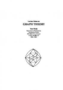
To be able to evaluate DOF the kinematical diagram of the mechanism has to be created. Diagrams should be drawn to scale proportional to the actual mechanism in the given position. The convention is to number links starting with the reference frame as number one while the joints should be lettered. The adopted strategy should consist of identifying on the real set of bodies: the frame, the actuator, and all the other links all joints any points of interest and draw the kinematical diagram according to the convention. Once we evaluated the mobility (degrees of freedom) we can identify the corresponding set of independent coordinates (parameters) and start the kinematical analysis of the mechanism


proceeding through the sub-task: a) define the reference frame (basic space in which the motion will be described) b) define the position of a point/particle with respect to the reference frame c) describe the type of motion (constrained or unconstrained) d) write the non-penetrating conditions e) define the independent coordinates f) find the velocity and acceleration A

1

Foundation

2

Crate

3

Pulley

4

Pulley

5

Motor/Actuator

6

Link

1 6 3

4 2 1

5

Joint analysis: A …. pin …. 2 dof

i = 3(6 − 1) − (5 ⋅ 2 + 3 ⋅1) The kinematical analysis of the whole set of connected bodies can be done if we would be able to describe the motion of each segment/body and then identify the kinematical quantities at the point of interest in the required position or time. Thus let’s start with the Kinematics of a Particle that is shown on the diagram as a point.


2

KINEMATICS OF A PARTICLE The position vector rA describes the position of a particle/point A, with respect to the reference frame (CS x,y,z). Character of a position vector depends on the arbitrary coordinate system At the instant the point A has a position r A = r (t ) = f (t )

during the time interval ∆t the point moves to a new position A1 that can be described by a position vector rA1 rA1 = rA + ∆r where: ∆r ....represents the position vector increment in time interval ∆s …represents the trajectory increment in time interval The Distance represents the measure of the point instant position with respect to the origin. Trajectory/path of the particular point is the loci of all instant positions of that point. The unit vector of the trajectory:

τ …unit vector in the tangent direction

τ = lim

∆t → 0

∆r dr = ∆s ds

then

d (xi + yj + zk ) = dx i + dy j + dz k ds ds ds ds dx dy dz where ds = cos α t ; ds = cos β t ; ds = cos γ t are the directional cosines of the tangent to the trajectory, and angles αt, βt, γt are the angles between axes x, y, z and the tangent vector τ τ=

n …unit vector in the normal direction to the trajectory has positive orientation towards the centre of the trajectory curvature ∆τ dτ n = lim = ∆t → 0 ∆ϑ dϑ taking into account the trajectory curvature radius R then

ds = R.dϑ and dτ dτ = R. . Substituting for τ we get ds ds R d 2r d 2x d2y d 2z n = R 2 = R 2 i + R 2 j+ R 2 k ds ds ds ds

thus n =


dϑ =

ds R

d 2x d2y d 2z = cos α ; = cos β ; = cos γ n are the directional cosines of the R R n n ds 2 ds 2 ds 2 normal to the trajectory, and αn; βn; γn are the angles between axes x, y, z and the normal

where: R

In case of 3D motion the trajectory is a 3D curve thus third unit vector in bi-normal direction has to be defined: b … unit vector in the bi-normal direction to the trajectory is oriented in a way that the positive direction of bi-normal vector forms together with normal and tangent right oriented perpendicular system. b = τ×n

2.1 VELOCITY Is the time rate of change of the positional vector. ∆r The average velocity of change is defined as v avr = ∆t Our interest is to find an instant velocity, that represents the limit case of average velocity. The time limit for computation of the instant velocity is approaching zero. ∆r dr The instant velocity is define as: v = lim = = rɺ ∆t → 0 ∆t dt What is the direction of the instant velocity? A common sense or rather to say intuition suggests that the velocity has the tangent direction to the trajectory. So let’s prove this statement mathematically: ∆r ∆ s ∆r ∆s dr ds ⋅ = lim ⋅ lim = ⋅ = τ ⋅ sɺ = τ ⋅ v ∆t → 0 ∆t ∆s ∆t → 0 ∆s ∆t → 0 ∆t ds dt

v = lim

since sɺ = lim

∆t → 0

∆s ds = =v ∆t dt

Having a positional vector defined as: r = xi + yj + zk then the velocity can be described by its components, since: v=

dr d dx dy dz = ( xi + yj + zk ) = i+ j + k = v x i + vY j + v Z k dt dt dt dt dt

where vx, vy, vz are components of the velocity in the direction of the axes of coordinate system. The magnitude/modulus of velocity: v = v 2x + v 2y + v 2z with directional cosines: cos α v =


vy vx v ; cos β v = ; cos γ v = z v v v

2.2 ACCELERATION The acceleration of a change of position is the time rate of change of velocity. To derive the expression for acceleration we need to draw velocity vector diagram so called velocity hodograph. Constructing hodograph based on the knowledge of path of a point and its velocity in particular position A and A1: Let’s have arbitrary point P through which both velocities vA, and vA1 will pass. The end points of their vectors are creating the desired curve hodograph. Based on hodograph

v A1 = v A + ∆v

∆v ∆t The instant acceleration is given as the limit value of average acceleration for time interval ∆t → 0 ∆v dv a = lim = = vɺ = ɺrɺ ∆t →0 ∆t dt

The average acceleration is given as

a avr =

The direction of acceleration can be found from

a=

dv d dτ dv = (τ ⋅ v ) = v+τ dt dt dt dt

dτ ds dv dτ ds dv dτ 2 dv Thus a = dt ⋅ ds ⋅ v + τ dt = ds ⋅ dt ⋅ v + τ dt = ds ⋅ v + τ dt dτ Since the direction of the normal is given as n = R. ds

then we can substitute

ρ represents the radius of the curvature at the instant. Therefore: v2 dv 1 a = n⋅ +τ⋅ = n ⋅ ⋅ sɺ 2 + τ ⋅ ɺsɺ = a n + a t ρ dt ρ Where

an = n ⋅

v2

ρ

is

the

acceleration in normal direction, and a t = τ ⋅ ɺsɺ is the tangential component of the acceleration.


dτ n = ds ρ

where

The direction of normal acceleration is always oriented to the center of instant curvature of the trajectory. The tangent component of acceleration captures the change of magnitude of a velocity while the normal component captures the change of direction of a velocity. at The resultant acceleration forms an angle β with normal direction: tan β = an Thus the acceleration expressed in the rectangular coordinate system would have form: dv d a= = ( v x i + v y j + vz k ) = a x i + a y j + a z k dt dt d a = ( xɺi + yɺj + zɺk ) = ɺɺ xi + ɺɺ yj + ɺɺ zk dt and the magnitude of acceleration:

a = a 2x + a 2y + a 2z

Orientation of the final acceleration is given by directional cosines: ay a a cos α a = x ; cos β a = ; cos γ a = z a a a and at the same time cos 2 α + cos 2 β + cos 2 γ = 1 Precise description of the motion of a particle is given by function capturing all kinematic quantities f (r , v, a t , a n , t ) = 0

2.2.1

Classification of motion

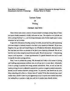
Consider the motion of the particle along the straight line (in the direction of x-axis). The tangential component of acceleration captures the change of velocity magnitude, thus it can be used to distinguish motion as:

Uniform motion Mathematical description: a t = 0 thus a t =

dv = 0 that implies v = const. dt

represents the simple differential equation solved by separation of t

x

variables v x ∫ dt = ∫ dx , thus giving 0

the solution

x0

x = x0 + v x ⋅ t

distance [m], velocity [m/s]

In case that the tangent takes the direction of axis x then v x = const. and equation v x =

60 50 40 30 20 10 0

distance traveled velocity

0

1

2

3

4

5 time [s]


6

7

8

9

10

dx dt

Uniformly accelerated/decelerated motion Mathematical description: a t = const. In case that the tangent takes the direction of axis x then a x = const. and t

v

0

v0

a x ∫ dt = ∫ dv x leading to solution at the same time v x =

dx therefore dt

ax =

dv x thus dt

v x = v0 + a x t t

x

0

x0

∫ (v0 + a x t )dt = ∫ dx

that gives the solution:

1 axt 2 2 The solution lead to an equation of trajectory of the point expressed as a function of time. x = x0 + v0 t +

Non-uniformly accelerated motion Mathematical description: a t = a x = a 0 ± kt (the function could be define differently) Thus a x ≠ const. =

dv x dt

therefore

t

v

0

v0

∫ (a0 ± kt )dt = ∫ dv x t

with solution x

1 2  ∫0  v0 + a0 t ± 2 kt dt = x∫ dx that gives the 0 1 1 trajectory equation x = x0 + v 0 t + a 0 t 2 ± kt 3 2 6

1 dx v x = v 0 + a 0 t ± kt 2 since v x = then 2 dt


Motion with other changes of kinematic quantities In this case the acceleration is given as a function of other quantities a = f (r , v, t )

2.3 ORTHOGONAL TRANSFORMATION You can see very clearly that velocity and acceleration directly depend on the positional vector. The positional vector form will vary according to the type of the coordinate system. Thus in rectangular coordinate system ( x, y, z ) the kinematical quantities in vector form are: r = rx i + ry j + rz k (positional vector)

d (rx i + ry j + rz k ) (velocity) dt d d2 a = a x i + a y j + a z k = (v x i + v y j + v z k ) = 2 (rx i + ry j + rz k ) dt dt

v = vx i + v y j + vzk =

(acceleration)

Let the point A be attached to the moving coordinate system x 2 , y 2 , z 2 with its origin coinciding with fixed coordinate system x1 , y1 , z1 ; O1 ≡ O2 The vector form of a position of the point A in CS1: r1A = r1Ax i 1 + r1Ay j1 + r1Az k 1 and in CS2:

r2A = r2Ax i 2 + r2Ay j 2 + r2Az k 2 A

or

r1AT = [x1

y1

z1 ]

and r2AT = [x 2

A

 x1   x2    A A in matrix form: r1 =  y1  and r2 =  y 2  ;  z1   z 2  y2 z2 ]

To express the positional vector r2A in CS1the vector has to be transformed. This process is called Orthogonal Transformation of Vector Quantities

2.3.1

Orthogonal Transformation of Vector Quantities

The mathematical operation is using matrix form of a vector. The CS1 is associated with basic frame/space that serves as a fixed reference frame that does not move. The moving point A is connected to the CS2, which moves with respect to the reference frame. Thus position of the point A in CS1 is r1A = x1A i 1 + y1A j1 + z1A k 1 r2A = x 2A i 2 + y 2A j 2 + z 2A k 2


and in CS2

How do we interpret positional vector r2A in CS1? The task is to project vector r2A into CS1. Thus projecting vector r2A into the x1 direction:

(

)

x1A = r2A ⋅ i 1 = x 2A i 2 + y 2A j 2 + z 2A k 2 ⋅ i 1

i1 ⇒ i 1 = i 2 ⋅ cos α 1 i2 i cosα 2 = 1 ⇒ i 1 = j 2 ⋅ cosα 2 j2 i cosα 3 = 1 ⇒ i 1 = k 2 ⋅ cosα 3 k2

where: cos α 1 =

x1A = x 2A i 2 ⋅ i 1 + y 2A j 2 ⋅ i 1 + z 2A k 2 ⋅ i 1 = x 2A i 2 i 2 cos α 1 + y 2A j2 j2 cos α 2 + z 2A k 2 k 2 cos α 3

Thus

x1A = r2A ⋅ i 1 = (x 2A i 2 + y 2A j 2 + z 2A k 2 ) ⋅ i 1 = x 2A cos α 1 + y 2A cos α 2 + z 2A cos α 3

( = (x

) k )⋅ k

y1A = r2A ⋅ j1 = x 2A i 2 + y 2A j 2 + z 2A k 2 ⋅ j1 = x 2A cos β 1 + y 2A cos β 2 + z 2A cos β 3 z1A = r2A ⋅ k 1

i + y 2A j 2 + z 2A

A 2 2

2

1

= x 2A cos γ 1 + y 2A cos γ 2 + z 2A cos γ 3

rewriting these three equations in matrix form will give

 x1   cos α 1 cos α 2  y  = cos β cos β 1 2  1   z1   cos γ 1 cos γ 2 A

cos α 1 where C 21 = cos β 1  cos γ 1

cosα 2 cos β 2 cos γ 2

cos α 3   x 2  cos β 3  ⋅  y 2  ⇒ r1A = C 21 ⋅ r2A cos γ 3   z 2  A

cos α 3  cos β 3  cos γ 3 

Analogically transformation from CS1 into CS2 gives: r2A = C12 ⋅ r1A where  cos α 1 T C12 = C 21 = cosα 2 cosα 3 and

cos β 1 cos β 2 cos β 3

cos γ 1  cos γ 2  cos γ 3 

C 21 ⋅ C T21 = I

The planar motion is special case when at any time of the motion z1 ≡ z 2

π

α1 = ϕ ;

α2 =

3π β1 = +ϕ ; 2

β2 = ϕ ;


2

+ ϕ ; α3 =

π

2 π β3 = 2

γ1 =

π 2;

and

γ2 = C 21

π

2; cos ϕ =  sin ϕ  0

γ3 = 0 − sin ϕ cos ϕ 0

0 cos ϕ 0 ≡  sin ϕ 1 

− sin ϕ  cos ϕ 

Once the positional vector is expressed in matrix form and the orthogonal transformation is used then the velocity and acceleration can be expressed in the same form.

2.3.2

Velocity in matrix form using the orthogonal transformation

Velocity is the first derivative of the positional vector d ɺ r A + C rɺ A v 1A = rɺ1A = (C 21r2A ) = C 21 2 21 2 dt If the point A does not change its position with respect to the origin CS2 then r2A=const. and ɺ ⋅rA therefore rɺ2A = 0 and v 1A = C 21 2

2.3.3

Acceleration in matrix form using the orthogonal transformation

Acceleration is the first derivative of the velocity and a second derivative of the positional vector, thus ɺɺ ⋅ r A + C ɺ ⋅ rɺ A + C ɺ ⋅ rɺ A + C ⋅ ɺrɺ A a1A = vɺ 1A = ɺrɺ1A = C 21 2 21 2 21 2 21 2 If the point A does not change its position with respect to origin CS2 then r2A=const. and ɺɺ ⋅ r A therefore rɺ2A = 0 and ɺrɺ2A = 0 thus giving a1A = C 21 2


PARTICLE IN CYLINDRICAL COORDINATE SYSTEM - r , ϕ , z

2.4 2.4.1

The position vector

in CS2 r2A = ρ ⋅ i 2 + z ⋅ k 2

ρ  In matrix form r =  0   z  A A Thus r1 = C 21 ⋅ r2 and since A 2

C 21 cos ϕ r = C 21 ⋅ r =  sin ϕ  0 A 1

A 2

cos ϕ =  sin ϕ  0 − sin ϕ cos ϕ 0

− sin ϕ cos ϕ 0 0 0 1

0 0 1

 ρ   ρ cos ϕ   0  =  ρ sin ϕ       z   z 2 

in vector form: r1A = ρ cos ϕ ⋅ i1 + ρ sin ϕ ⋅ j1 + z ⋅ k1

2.4.2

The velocity

dr d = ( ρ ⋅ i 2 + z ⋅ k 2 ) = ρɺ ⋅ i 2 + ρ ⋅ ɺi 2 + zɺ ⋅ k 2 + z ⋅ kɺ 2 dt dt where unit vector k2 remains constant (magnitude as well as direction does not change with time), therefore kɺ 2 = 0 Expressed in vector form

v 2A =

The unit vector i2 rotates in the plane x, y around the origin thus the velocity is given as di dρ dz v 2A = i2 + ρ 2 + k2 where dt dt dt di 2 dϕ = × i 2 = ω z × i 2 = j 2 ⋅ ω represents the transverse vector perpendicular to unit vector i2. dt dt dρ dϕ dz Thus the velocity v 2A = i2 + ρ j2 + k 2 = ρɺ ⋅ i 2 + ϕɺ ⋅ ρ ⋅ j2 + zɺ ⋅ k 2 dt dt dt Where ρɺ ⋅ i 2 = v ρ represents the radial component of velocity

ϕɺ ⋅ ρ ⋅ j2 = vt represents the transverse component of velocity zɺ ⋅ k 2 = v z represents the z-component of velocity in matrix form: the transpose velocity in CS2 v T2 = [ρɺ

in CS1

cos ϕ v = C 21 ⋅ v =  sin ϕ  0 A 1


A 2

− sin ϕ cos ϕ 0

ρϕɺ

zɺ ]

0  ρɺ   ρɺ cos ϕ − ρω sin ϕ  0 ⋅  ρϕɺ  =  ρɺ sin ϕ + ρω cos ϕ   1   zɺ   zɺ

2.4.3

The acceleration

in vector form

a 2A =

(

)

dv d d = ρɺ ⋅ i 2 + ρ ⋅ ɺi 2 + zɺ ⋅ k 2 = ( ρɺ ⋅ i 2 + ρ ⋅ ϕɺ ⋅ j2 + zɺ ⋅ k 2 ) dt dt dt

a 2A = ρɺɺ ⋅ i 2 + ρɺ ⋅ ɺi 2 + ρɺ ⋅ ϕɺ ⋅ j2 + ρ ⋅ ϕɺɺ ⋅ j2 + ρ ⋅ ϕɺ ⋅ ɺj2 + ɺɺ z ⋅k2

a 2A = ρɺɺ ⋅ i 2 + ρɺ ⋅ ω ⋅ j2 + ρɺ ⋅ ω ⋅ j2 + ρ ⋅ α ⋅ j2 + ρ ⋅ ω ⋅ ɺj2 + ɺɺ z ⋅k2 dj 2 = ω z × j 2 = −i 2 ⋅ ω dt z ⋅k2 Thus giving acceleration a 2A = ρɺɺ ⋅ i 2 + 2 ρɺ ⋅ ϕɺ ⋅ j2 + ρ ⋅ ϕɺɺ ⋅ j2 − ρ ⋅ ω 2i 2 + ɺɺ where:

a 2A = ( ρɺɺ − ρ ⋅ ϕɺ 2 )i 2 + ( ρ ⋅ ϕɺɺ + 2 ρɺ ⋅ ϕɺ ) j2 + ɺɺ z ⋅k2 where

( ρɺɺ − ρϕɺ 2 ) = a ρ

represents the radial acceleration ɺ ( ρϕɺɺ + 2 ρϕɺ ) = a p represents the transverse acceleration ɺzɺ = a z represents the acceleration in the z-axis direction

in matrix form:

a 2AT =  ρɺɺ − ρ ⋅ ϕɺ 2 ρ ⋅ ϕɺɺ + 2 ρɺ ⋅ ϕɺ ɺɺ z   2 cos ϕ − sin ϕ 0  ρɺɺ − ρϕɺ    a1A = C 21a 2A =  sin ϕ cos ϕ 0  ρϕɺɺ + 2 ρɺϕɺ    0 ɺzɺ 0 1   In this presentation we associated angle ϕ with angular vector coordinate thus angular velocity ϕɺ = ϕɺ ⋅ k1 = ω ⋅ k1 = ω and angular acceleration ϕɺɺ = ϕɺɺ ⋅ k1 = ωɺ ⋅ k1 = α

2.4.4

Special cases

a) z=0 , ρ = const., ϕ (t) The particle (the point A) is restricted to the plane x,y only and moves in a way that the trajectory of the point A is a circle in the plane x,y. The velocity and acceleration expressed in general coordinates in the previous paragraph is: A v 2 = ρɺ ⋅ i 2 + ϕɺ ⋅ ρ ⋅ j2 + zɺ ⋅ k 2

a 2A = ( ρɺɺ − ρ ⋅ ϕɺ 2 )i 2 + ( ρ ⋅ ϕɺɺ + 2 ρɺ ⋅ ϕɺ ) j2 + ɺɺ z ⋅k2 Thus for our particular case in CS2: v 2A = ϕɺ ⋅ ρ ⋅ j2 in CS1: v1A = − ρ ⋅ ϕɺ sin ϕ ⋅ i1 + ϕɺ ⋅ ρ cos ϕ ⋅ j1 18 Dr. Ing. Zdenka Sant 10/2009

ϕ = ϕ ⋅ k1 = ϕ ⋅ k 2

A 2 and acceleration in CS2: a 2 = − ρ ⋅ ϕɺ i 2 + ρ ⋅ ϕɺɺ ⋅ j2 A 2 where a 2 n = − ρ ⋅ ϕɺ i 2 represents the normal acceleration oriented always towards the centre of curvature of the trajectory a 2Aτ = ρ ⋅ ϕɺɺ ⋅ j2 represents the tangential component of an acceleration

in CS1: where

a1A = ( − ρ ⋅ ϕɺ 2 cos ϕ − ρ ⋅ ϕɺɺ sin ϕ )i1 + ( ρ ⋅ ϕɺɺ cos ϕ − ρ ⋅ ϕɺ 2 sin ϕ ) j1 − ρ ⋅ ϕɺ 2 cos ϕ = anx is the x-component of the normal acceleration in CS1 − ρ ⋅ ϕɺɺ sin ϕ = aτ x is the x-component of the tangential acceleration in CS1

ρ ⋅ ϕɺɺ cos ϕ = aτ y is the y-component of the tangential acceleration in CS1 − ρ ⋅ ϕɺ 2 sin ϕ = any is the y-component of the normal acceleration in CS1 b) z=0 , ρ(t), ϕ(t) The particle (point) moves in the plane x,y and description of the problem uses polar coordinates (ρ,ϕ)

2.5 PARTICLE TRAJECTORY The motion could be classified with respect to the trajectory as:

2.5.1

Rectilinear motion

The position of a point is described as a function of curvilinear coordinates s : r = r(s) dr where τ2 = 1 =τ ds and The necessary condition for rectilinear motion is given as: τ = const. The velocity is given as: dr dr ds dr ds v= = ⋅ = ⋅ = τ ⋅ sɺ dt dt ds ds dt and acceleration: a = If:

sɺ = const . therefore ɺsɺ = 0 …uniform rectilinear motion ɺsɺ ≠ 0 …..accelerated rectilinear motion sɺ ≠ const. thus for ɺsɺ = const. then uniformly accelerated rectilinear motion for ɺsɺ ≠ const . then non-uniformly accelerated rectilinear motion


dv d = ( τ ⋅ sɺ) = τ ⋅ ɺɺ s dt dt

2.5.2

Curvilinear motion

In case of curvilinear motion r = r(s) and and velocity is expressed as:

v=

s = s(t)

dr dr ds dr ds = ⋅ = ⋅ = τ ⋅ sɺ dt dt ds ds dt

Where τ 2 = 1 as well as τ ≠ const. since the unit vector changes its direction The acceleration is: a=

dv d 1 = ( τ ⋅ sɺ) = τ ⋅ ɺɺ s + n ⋅ sɺ 2 = aτ + a n dt dt ρ

In case that: a) sɺ = const. therefore

then ɺsɺ = 0 1 a = n sɺ 2 = a n and the point moves along the circular trajectory with uniform

ρ

velocity . b) sɺ ≠ const .

then

ɺsɺ ≠ 0 and motion is non-uniformly accelerated or sɺ 2 ɺsɺ = const . where a = τɺsɺ + n motion is uniformly accelerated

ρ

2.6 HARMONIC MOTION The motion of a point (particle) that is described by equation x = A sin(ω ⋅ t + ϕ )

A

represents the amplitude (max. deviation from neutral position) [m] ω represents the angular frequency [s-1] ϕ represents the phase shift [rad] x represents the instant distance of the particle is called the harmonic motion dx Velocity is in this case is given as: v = = A ⋅ ω cos(ω ⋅ t + ϕ ) and dt dv Acceleration is given by: a = = − A ⋅ ω 2 sin(ω ⋅ t + ϕ ) dt where

For the initial condition: t = 0, x = x0, v = v0, a = a0 the kinematical quantities are:

x0 = A sin ϕ


;

v 0 = Aω cos ϕ

;

a 0 = − Aω 2 sin ϕ

Graphical interpretation of harmonic motion can be represented as the rectification of all kinematical quantities in time

harmonic motion distamce x [m]

x, v , a

instant vlocity v [m/s]

tim e

ωT = 2π 2π

1 [Hz] T ω Amplitude of the motion can be expressed from x0 = A sin ϕ and v 0 = Aω cos ϕ

Where T represents the period T =

A = x 02 +

v 02

ω

2

and

[s] thus frequency f =

tan ϕ =

sin ϕ x0ω = cos ϕ v0

Thus the kinematical quantities can be expressed as function of rotating vector rx, rv, ra Where

|rx| = A; |rv| = Aω; |ra| = Aω2


4

3.8

3.6

3.4

3.2

3

2.8

2.6

2.4

2.2

2

1.8

1.6

1.4

1.2

1

0.8

0.6

0.4

0.2

instant accel. [m/s^2]

0

2.5 2 1.5 1 0.5 0 -0.5 -1 -1.5 -2 -2.5

2.6.1

Composition of harmonic motions in the same direction

a) If ω1 = ω2 = … = ωn = ω then x1 = A1 sin(ωt + ϕ 1 ) = A1e i (ωt +ϕ1 ) x 2 = A2 sin(ωt + ϕ 2 ) = A2 e i (ωt +ϕ 2 ) . .

x n = An sin(ωt + ϕ n ) = An e i (ωt +ϕ n ) The resulting motion is again harmonic motion described as: n

n

n

j =1

j =1

j =1

x = ∑ x j = ∑ A j sin(ω ⋅ t + ϕ j ) = ∑ A j e

i (ω ⋅t +ϕ j )

n

= ∑ A j eiω t ⋅ e

iϕ j

j =1

= eiω t ∑ A j e

iϕ j

thus

x = Av ei (ω ⋅t +ϕv ) substituting for t = 0 we get :

x = Av e iϕ v from where we get the final amplitude and phase shift n

n

j =1

j =1

Av = (∑ A j cos ϕ j ) 2 + (∑ A j sin ϕ j ) 2 n

∑A and ϕ v =

j =1

j

sin ϕ j

j

cos ϕ j

n

∑A j =1

b) If ω1 ≠ ω2 ≠ .... ≠ ωn

then each motion is described by its own equation

x1 = A1 sin(ω1 ⋅ t + ϕ1 ) = A1ei (ω1 ⋅t +ϕ1 ) x2 = A2 sin(ω 2 ⋅ t + ϕ 2 ) = A2ei (ω2 ⋅t +ϕ 2 )

xn = An sin(ω n ⋅ t + ϕ n ) = An ei (ωn ⋅t +ϕ n ) and the final motion is described by equation: n

n

n

j =1

j =1

j =1

x = ∑ x j = ∑ A j sin(ω j t + ϕ j ) = ∑ A j e

i ( ω j t +ϕ j )

The final motion composed from harmonic motions with different angular frequencies is not a harmonic motion, since the resulting amplitude is not constant. 2πn1 2πn2 ω n In case that ω1 = and ω 2 = and at the same time the ratio 1 = 1 is a rational T T ω 2 n2 number the resulting motion is said to be periodic motion.


2.6.2

Composition of two perpendicular harmonic motions

The motion of two particles moving in two perpendicular directions is defined by equations: x = A1 sin(ω1t + ϕ 1 ) = A1e i (ω1t +ϕ1 ) and y = A2 sin(ω 2 t + ϕ 2 ) = A2 e i (ω 2t +ϕ 2 ) These equations define curves known as Lissajous picture. The solution is quite demanding and beyond our scope. The relatively simple solutions exists for special cases, when ω1 = ω2 and assumption A1 = A2 leading to equation of ellipse on conjugate axes.

2.7 MOTION OF A SET OF PARTICLES Set of particles can be either connected set or particles or number of two or more unconnected particles moving in the same reference system. Thus the relationship between particles has to be taken into consideration. Let’s take the case of particle A and B as shown on diagram: Both particles are connected via inextensible cable carried over the pulleys. This imposes non-penetrable condition between them: l = s A + h + 2 ( h − sB ) The additional length of the cable between the upper datum and the ceiling as well as the portion of the cable embracing the pulleys will remain constant during the motion thus does not play any role in the kinematical description. Investigating mobility of the set of particles would define the number of independent coordinates that in our case is i = 1 The path of a particle A is not identical with path of the particle B and the relation between them has to be described based on the joints involved. Thus except of the nopenetration condition the support at A has to be taken into consideration as well as the supports for the pulleys and body B. Having the basic condition of the inextensible length we can evaluate the relation between velocities of the particle A and B as a time derivative of the l. Thus 0 = v A + 2 ⋅ vB Then we can conclude that for motion of the particle A in positive direction (away from the datum v in the direction of sA) the particle B will move upwards with velocity vB = A . 2 23 Dr. Ing. Zdenka Sant 10/2009

3

SOLID BODY MOTION

As we announced before the model body adopted in kinematics is again non-deformable, therefore the distance between two points A, B on a solid body will follow the rule mathematically expressed as: AB = const.

3.1 TRANSLATION MOTION OF A SOLID BODY The position and trajectory of two points A, B is investigated. If two moving points will draw their trajectory in two parallel planes, thus their trajectories are parallel curves. The change of position from point A to A’ and B to B’ is described by vectors p that are parallel. The advance motion is rectilinear (solid line) if vector p is a straight line and curvilinear if it is a curve (dotted line). The change of position of the point A is rA ' = rA + p of the point B

rB' = rB + p

Thus

rA ' − rA = rB' − rB

or rearranged

rB − rA = rB' − rA '

Expressing vectors rB and rB’with respect to the reference point A/A’ we can prove previous statement about parallel vectors rBA = rB’A’ = const.

3.1.1

Investigating kinematic quantities

Position Point A is the reference point attached to the body associated with moving CS2 (x2, y2, z2). Position of a point B is given as r1B = r1A + r1BA and

r1BA = x 2BA cos α 1 + y 2BA cos α 2 + z 2BA cos α 3


thus the position of the point B in CS1 is x1B = x1A + x 2BA cos α 1 + y 2BA cos α 2 + z 2BA cos α 3 y1B = y1A + x 2BA cos β 1 + y 2BA cos β 2 + z 2BA cos β 3 z1B = z1A + x 2BA cos γ 1 + y 2BA cos γ 2 + z 2BA cos γ 3

or in matrix form r1B = r1A + C 21 ⋅ r2BA Transformation matrix C21 contains the cosines of all angles among axes of coordinate system. Since all vectors remain parallel vectors the angles between particular axes are constant. Therefore C 21 = const.

Velocity In vector form the velocity of point B is given as: dr B d v 1B = 1 = (r1A + r1BA ) = v 1A + v 1BA = v 1A since the r1BA = const. dt dt

ɺ ⋅ r BA + C ⋅ rɺ BA In matrix form : v 1B = rɺ1B = rɺ1A + C 21 2 21 2 ɺ and C 21 = 0 since C 21 = const. Thus the final matrix form is:

v 1B = rɺ1B = rɺ1A = v 1A

Acceleration In vector form the acceleration of point B is given as: dv B d a1B = 1 = ( v1A + v1BA ) = vɺ 1A = a1A since v1BA = 0 dt dt In matrix form :

a1B = ɺrɺ1B = vɺ 1B = v 1A = a1A

3.2 ROTATION OF A SOLID BODY AROUND FIXED AXIS If two points of a moving solid body are stationary then v O1 = v O 2 = 0 then the solid body rotates around axis that passes through these points O1 and O2. The positional vectors describe their position in CS1 by rO1 = const., rO2 = const.


Any point on the line specified by points O1 and O2 can be described as rO3 = rO1 + λrO2O1 and the velocity of point O3 is obtained by the first derivative of its position, thus rO3 = v O3 = 0

Conclusion: There are infinity of points, laying on the line specified by points O1 and O2, which have a zero velocity. The loci of all points that have a zero velocity is called the axis of rotation. The path of a point A that lays in the plane (x,z) rotating around the axis z, is a circle with radius ρ, which corresponds to the projection of the position vector rA into the x,y plane. The instant position of a point A depends on the instant angle of rotation ϕ = ϕ(t) further on we assign to this angular coordinate a vector quantity that follows the right hand rule. The angular velocity that describes the rate of change of angular coordinate is expressed as ∆ϕ the average value of angular velocity: ω aver = ∆t ∆ϕ dϕ = =ω ∆t → 0 ∆t dt

The instant angular velocity is given as: lim

In the same way we can express the angular acceleration. ∆ω The average acceleration is given as : α aver = and ∆t Instant thus

acceleration

ɺ = e ϕ ϕɺɺ α=ω

is

lim

∆t → 0

∆ω dω = =α ∆t dt

If the solid body rotates around fixed axis then all point of the body have the same angular velocity and acceleration.

3.2.1

Finding the velocity of an arbitrary point

The point B is attached to the rotating solid body Then the position of a point B in CS2 is given as r2B = x2B i 2 + y2B j2 + z 2B k 2


thus

ω = ϕɺ = e ϕ ϕɺ

or with respect to the point O’ around which the point B rotates with radius ρ

r2B = r2O + ρ '

Point B moves on the circular trajectory in time ∆t →0 a distance dr = dϕ ⋅ ρ = dϕ ⋅ rB ⋅ sin β dr = dϕ × rB = dϕ × ρ in vector form: since vectors r and ρ lay in the same plane and together with vector ϕ form the plane to which the path increment dr is orthogonal (perpendicular). Thus the velocity of the point B is dr dϕ dϕ vB = = × rB = × ρ = ω × rB = ω × ρ dt dt dt

v B = ω ⋅ rB ⋅ sin β = ω ⋅ ρ

the module of velocity: or in vector from:

i

k

ry

rz

ω y ω z = i (ω y rz − ω z ry ) + j(ω z rx − ω x rz ) + k (ω x ry − ω y rx )

v B = ω × rB = ω x rx then

j

v B = iv x + jv y + kv z

with module

v B = v x2 + v y2 + v z2

The orientation of the linear velocity is given by right hand rule: Grabbing the axis of rotation with our right hand in a way that the thumb points in the direction of angular velocity then fingers would show the direction of velocity of the particular point of a body. If the position of the point B is expressed in matrix form r1B = C 21 ⋅ r2B then the velocity is the first derivative of position, thus

d (C 21r2B ) = Cɺ 21r2B + C 21rɺ2B dt Since the point B is attached to and rotates with CS2 then

v 1B = rɺ1B =

r2B = const. and its first derivative is equal to zero. ɺ rB = Ω ⋅C ⋅rB The velocity of the point B is given as v 1B = rɺ1B = C 21 2 1 21 2 The first derivative of transformation matrix and finally

3.2.2

v 1B = Ω 1 ⋅ C 21 ⋅ r2B = C 21 ⋅ Ω 2 ⋅ r2B

Finding the acceleration of an arbitrary point B

In vector form:

and simultaneously 27 Dr. Ing. Zdenka Sant 10/2009

ɺ = Ω C = C ⋅Ω C 21 1 21 21 2

a B = vɺ B =

d (ω × rB ) = α × rB + ω × v B dt

aB =

d (ω × ρ ) = α × ρ + ω × v B dt

Since the point B moves on the circular path the acceleration will have two components Tangential component i j k aτB = α × ρ = α × rB = α x

α y α z = i (α y rz − α z ry ) + j(α z rx − α x rz ) + k (α x ry − α y rx )

rx

and normal acceleration i j a = ω × vB = ωx n B

vx

ry

rz

k

ω y ω z = i (ω y v z − ω z v y ) + j(ω z v x − ω x v z ) + k (ω x v y − ω y v x ) vy

vz

Their modules are: aτB = ( a τx ) 2 + (a τy ) 2 + ( a τz ) 2

and

a

n B

= (a ) + (a ) + (a ) n 2 x

n 2 y

n 2 z

or

a

n B

or

aτB = αrB sin β = αρ

= ωv B = ω ρ = ω rB = 2

2

v B2

ρ

In matrix form:

ɺɺ ⋅ r B + 2C ɺ ⋅ rɺ B + C ⋅ ɺrɺ B a 1B = vɺ 1B = ɺrɺ1B = C 21 2 21 2 21 2

which leads to

ɺɺ ⋅ r B a 1B = vɺ 1B = ɺrɺ1B = C 21 2

then the second derivative of transformation matrix is:

ɺɺ = Ω ɺ C +Ω C ɺ C 21 1 21 1 21 ɺɺ = Ω ɺ C +Ω Ω C = Ω ɺ C + Ω 2C C 21 1 21 1 1 21 1 21 1 21 ɺɺ = A C + Ω 2C C 21 1 21 1 21 Thus the acceleration of the point B is a1B = ( A 1C 21 + Ω12 C 21 )r2B = ( A 1 + Ω12 )C 21r2B = ( A 1 + Ω12 )r1B

where the first component represents the tangential acceleration  0 −α z  Bτ B B a1 = A 1C 21r2 = A 1r1 = A 1ρ where A =  α z 0 − α y α x 

αy   −α x  0 

and the second component represents the normal acceleration n

a1B = Ω1 C 21r2B = Ω1 r1B = Ω1 v 1B 2

2

The course of motion is recorded by the tangential acceleration α τ = α ⋅ ρ dω where α = = ωɺ dt


There could be two situations: ω = const. ⇒ α = 0

a)

a n = ρ ⋅ω 2 =

Thus a τ = 0 and

v2

ρ

These characteristics represent uniform motion of the particle on the circle and the acceleration that occurs is the normal acceleration. b) ω ≠ const. ⇒ α ≠ 0 In this case the angular acceleration α can become: i)

α = const.

thus

α τ = α ⋅ ρ = const. (assuming ρ = const.)

These characteristics represent uniformly accelerated motion on the circular path – uniformly accelerated rotation. ii)

α ≠ const.

thus

α τ ≠ α ⋅ ρ ≠ const.

These characteristics represent non-uniformly accelerated motion on the circle, non-uniformly accelerated rotation. v2 In both cases the normal acceleration will occur. a n = ρ ⋅ ω 2 =

ρ

3.2.3

Solid body kinematics consequences (the geometrical dependency)

Providing the graphical solution for kinematic quantities, we need to record velocity and acceleration in a graphical form. For this purpose the length and velocity scale has to be given, while the remaining scales are calculated. Where lρB represents the length of the radius vector ρ

ρ

thus ρ = sl ⋅ l ρ sl and velocity v = s v ⋅ l v lρ =

Therefore the angle αv is given as l v s tan α v = v = ⋅ l = ω ⋅ k v l ρ ρ sv where kv is a velocity scale constant. Since all points on the body have the same angular velocity ω we can conclude - Sentence about velocities: All arrowheads of velocity vectors, for particular points of a rotating body, are visible from the fixed point of rotation (v=0) under the same angle αv at the instant instant moment. 29 Dr. Ing. Zdenka Sant 10/2009

Acceleration – the graphical solution A tangential and normal components of acceleration has to be recorded The normal component of acceleration: v2 a n = ρ ⋅ω 2 = thus from Euclid’s law about the height in the triangle follows

ρ

the graphical construction of normal acceleration. The acceleration scale has to be calculated!! s2 ⋅l2 Therefore a n = v v = s a ⋅ l an where sl ⋅ l ρ

l an =

l v2 lρ

sa =

and

s v2 sl

The tangential component of acceleration: α τ = α ⋅ ρ The direction of tangential component corresponds to the direction of velocity hence further analogy with velocity is obvious. la a s tan α aτ = τ = τ ⋅ l = α ⋅ k aτ ρ sa lρ where kaτ is a tangential acceleration scale constant. Since all points on the body have the same angular acceleration α we can conclude: Sentence about tangential acceleration: All arrowheads of tangential acceleration vectors, at the points on the rotating body, are at the instant visible under the same angle αaτ from the fixed point of rotation (v=0). τ

The total acceleration is given as a sum of its components a = a + a αρ α aτ tan β = n = 2 = 2 = k a a ω ρ ω

n

where ka represents the scale constant of total acceleration. Since α and ω are constant for all points on the body we conclude: The total acceleration of the point on the rotating solid body makes an angle β from its normal to the trajectory that remains constant for all points on the body. And finally we can finalise based on the background:

tan α a =

l aτ l ρ − lan

=

α ma m − ω 2 −1 l

together with the angular kinematic quantities α, ω that are the same for all points of the body: All arrowheads of total acceleration vectors of all points on the rotating body, are at the instant visible under the same angle αa from the fixed point of rotation (v=0).


3.3 UNIVERSAL PLANAR MOTION If all points of a body move in planes parallel to the fixed (stationary) basic plane then we say that the body moves in planar motion. If the trajectories of all points that lay on the line perpendicular to that plane are planar curves then the motion is a universal planar motion. The initial position of the body is described via points A, B. A positional vector for point B using a reference point A describes the initial position of a body: r B = r A + r BA During the time interval t their position changes to a new location A1 and B1 thus r B1 = r A1 + r B1 A1 As seen on the diagram r BA ≠ r B1 A1 but r BA = r B1 A1

,

which

means that the vector changes its orientation but not its magnitude. Therefore we can imagine the universal planar motion as a sequence of translation motion followed by rotation that could be expressed in a short way as: GPM = TM + RM Note: Both motion are happening in the same time and this approach is just imaginary.

3.3.1

The position

of the point B can be expressed in vector or matrix form: r1B = r1A + r1BA with use of transformation matrix C21: r1B = r1A + C 21 ⋅ r2BA

that leads to two equations in vector form: x1B = x1A + x 2BA cos ϕ − y 2BA sin ϕ y1B = y1A + x 2BA sin ϕ + y 2BA cos ϕ or in matrix form:

 x1B   x1A   B  A  y1  =  y1  +  z1B   z1A      31 Dr. Ing. Zdenka Sant 10/2009

cos ϕ  sin ϕ   0

− sin ϕ cos ϕ 0

0  x 2BA    0  y 2BA  1  z 2BA 

3.3.2

The velocity

of a point B can be expressed: in vector form: thus or in matrix form:

v 1B =

(

)

d A r1 + r1BA = v 1A + v 1BA dt

v 1B = v 1A + ω × r1BA

ɺ r BA v 1B = v 1A + v 1BA = v 1A + C 21 2 v 1B = v 1A + Ω1C 21r2BA = v 1A + Ω1r1BA

There is a rotation of the point B with respect to the point A thus we say that there is a relative motion of the point B around point A. Thus

v 1BA = ω × r1BA

where ω represents the angular velocity of a relative motion with respect to the point A. v BA v CA ω = = = const. The relative angular velocity is constant for all points of the body thus: BA C A Then we can get the components of velocity:

v xB  v xA   0  B  A  v y  = v y  + ω  0   0   0  1  1

−ω 0 0

0  x BA    0  y BA  0  0  1

Graphical solution: The velocity of a point A is known, thus we need to find the velocity at the point B based on the vector equation: v 1B = v 1A + ω × r1BA


3.3.3

The pole of motion

If ω ≠ 0 then there exists just one point on the body that has zero velocity at the instant and belongs to the moving body (or the plane attached to the moving body). This point is known as the instantaneous centre of rotation or the pole of motion. The position of a pole P is given as: r1P = r1A + r1PA

in matrix form:

ɺ r PA r1P = r1A + r1PA = r1A + C 21 2 v1P = v 1A + v 1PA

Then the velocity of the pole is:

since the linear velocity at this location is zero, then

0 = v1A + v1PA → v1PA = − v1A For arbitrary reference point we would get similar answer: 0 = v 1B + v 1PB → v 1PB = − v 1B To find a position of the pole of a body moving with GPM we have to multiply the velocity equation by the angular velocity 0 = ω × v 1A + ω × (ω × r1PA )

Thus

0 = ω × v 1A + [ω ⋅ (ω ⋅ r1PA ) − r1PA ⋅ (ω ⋅ ω)]

Rearranging the equation into a form ω ⋅ r1PA = 0

while equating

ω ⋅ω = ω 2

and

0 = ω × v 1A + ( −ω 2 r1PA )

we get

from where we equate the pole positional vector

PA 1

r

=

ω × v 1A

ω2


=

ω × τv1A

ω2

 i1 1  = 20 ω v xA 

j1

0 v yA

k1  1  ω  = 2 i 1 (−ωv yA ) + j1 (ωv xA ) ω 0 

[

]

Graphical solution: Based on v 1PA = − v 1A and v 1PB = − v 1B The velocity vA is known and velocity at the point B is v 1B = v 1A + v 1BA thus if we know the velocity we know the direction of a normal to the trajectory.

The pole of motion is at the intersection of normal nA and nB.

Finding the velocity by means of the pole r1B = r1P + r1BP

Position of a point B

r1B = r1P + C 21r2BP

or

v 1B = v 1P + Ω1C 21r2BP

Then the velocity is:

Since the velocity of the pole is zero we get v 1B = Ω1C 21r2BP

in matrix form

 vxB   0  B   v y  = ω  0   0  1

−ω 0 0

0   cos ϕ 0   sin ϕ 0 1  0

− sin ϕ cos ϕ 0

that would result in B v1x = −ωy1BP

B v1y = ωx1BP

and

Thus giving the final velocity

v 1B =

(v ) + (v ) B 2 1x

B 2 1y

Then the angular velocity is

=

(− ωy ) + (ωx ) BP 2 1

ω=

BP 2 1

=ω

(y ) + (x ) BP 2 1

v1B r1BP

From this result follows the interpretation for graphical solution:

ω=

s ⋅l v1B = v v = k v ⋅ tan α v BP sl ⋅ l r BP r1


tan α v =

thus giving

1 ω kv

BP 2 1

= ωr1BP

0   x BP    0   y BP  1   0 

2

Conclusion: All arrowheads of velocity vectors, for particular points of a rotating body, are visible from the instantaneous centre of rotation rotation (vP=0) under the same angle αv at the instant moment.

3.3.4

Finding the acceleration

Analytically We have already found the positional vector r1B and velocity v1B

r1B = r1A + r1BA v 1B = v 1A + v 1BA where the velocity v1BA represents the relative motion of the point B around the point A that can be expressed as

v 1BA = ω × r1BA

in vector form or

v 1BA = Ω1C 21r2BA = Ω1r1BA in matrix form. Since we proved that we can derive the equation of acceleration

a = ɺrɺ = vɺ

a1B = a1A + a1BA

Where the acceleration of relative motion of a point B around point A will have two components since the relative motion is the rotation with a fixed point at A.

a1BA = α × r1BA + ω × v 1BA Thus result of derivation:

in vector form. The acceleration in the matrix form is a

r1B = r1A + r1BA = r1A + C 21 ⋅ r2BA v 1B = v 1A + Ω1 ⋅ C 21 ⋅ r2BA ɺ ⋅ C ⋅ r BA + Ω ⋅ C ɺ ⋅ r BA + Ω ⋅ C ⋅ rɺ BA a1B = a1A + Ω 1 21 2 1 21 2 1 21 2 BA in case of solid body rɺ2 = 0 since the distance between points A and B does not change, thus

a1B = a1A + A 1 ⋅ C 21 ⋅ r2BA + Ω1 ⋅ Ω1 ⋅ C 21 ⋅ r2BA

a1B = a1A + ( A 1 + Ω1 ) ⋅ r1BA 2

 0  where A 1 =  α z − α y  acceleration 35 Dr. Ing. Zdenka Sant 10/2009

−α z 0

αx

αy   −αx  0 

represents the half symmetrical matrix of angular

Graphically To find the acceleration we will use the leading equation

a1B = a1A + a1BA The acceleration of a point A is given and acceleration of the relative motion of point B is described by two components (tangential and normal) in the respective directions to the path of the point B. The normal component of the acceleration aBA is found from the known velocity vBA (graphically by means of Euclid triangle). Thus at the instant moment the angle β between the final acceleration of the relative motion and the normal to the path of relative motion is given by a BA α tan β = τBA = 2 = const. an ω Conclusion:

The final acceleration of the relative motion around point A makes an angle β with the normal component of the acceleration that is constant for all points of the body moving with relative motion. In a similar way we can observe the tangential component of acceleration and the final acceleration. Thus this angle is given by:

tan α a =

l a BA τ

l ρ − l a BA n

=

l v2 α ⋅ s l ⋅ s v2 = . where l ρ la s a ( s v2 − ω 2 sl2 ) n

Since α and ω are constant in the given time interval for all points of the rigid body then even the tanαa=const. Conclusion: The end points of tangent components of acceleration for all points on the body are seen from the centre of rotation under the same angle αa at the instant moment.


3.3.5

The instantenous centre of acceleration – the pole of acceleration

Similarly as for the pole of velocity P there is a pole of acceleration Q, the point that has zero acceleration at the instant. The acceleration for this pole Q is given by: QA a1Q = a1A + a1QA τ + a 1n

a1Q = a1A + α × r1QA + ω × (ω × r1QA )

Multiplying by α from left 0 = α × a1A + α × (α × r1QA ) + α × [ω × (ω × r1QA )] we receive 0 = α × a1A + (−α 2 )r1QA + (−ω 2 )(α × r1QA ) and substituting for the expression α × r1QA = −a1A − (−ω 2 r1QA ) = −a1A + ω 2 r1QA

we

find

the

positional vector of pole of acceleration α × a1A + ω 2 a1A r1QA = α 2 +ω4 Comparing this expression with the expression for pole of velocity ω × v 1A r1PA = 2

ω

shows that these two expressions are different, thus the two poles are different and we can conclude: The pole of acceleration is not identical with pole of velocity If ω ≠ 0 and α ≠ 0 then there is one point on the moving plane that has acceleration aQ=0. This point lays at the intersection of lines that make an angle β with the directions of total acceleration of each and every point on the moving plane.


3.4 CENTRE OF THE TRAJECTORY CURVATURE The body, moving with the universal planar motion, is defined by two points A and B and their trajectories sA and sB that the points are drawing in the plane. Thus the position of the pole of velocity that lies in the intersection of two normals can found at any instant. The body is connected to the moving CS2 and the positions of all instantaneous poles of velocity are creating a curve pH – the locus of all such positions is called the moving polode while the poles connected to the stationary fixed plane CS1 are creating a curve assigned the symbol pN – the fixed polode. Thus we can imagine the universal planar motion as motion created by rollingof the locus of poles pH (associated with moving plane) on the locus of poles pN (associated with the fixed frame). The pole velocity describes the rate of change of the pole position. It is possible to find the rate of change of the positional vector using the reference point A with respect to the fixed frame ω×aA − α× vA P A vN = v + 2

ω

And for the pole associated with the moving plane

v PH = v A +

ω×aA −α× vA

ω2

Since the derived equations of pole velocities are identical we can assign a symbol vπ to be its pole of velocity and conclude:

The point where both loci pN and pH touch at the instant is the pole of motion P (the instantaneous centre of rotation) and at this point the two curves have a common tangent tp. The pole velocity as the rate of change of the pole position will lie on the tangent tp.


The task is to investigate the velocity and acceleration of the point or define the velocity and acceleration of the whole body. The points of the moving body are drawing trajectories thus at the instant each point of the body is characterized by its normal to the motion and the radius of its trajectory. While constructing the normal component of acceleration 1 n sɺ 2 = a n

ρ

the centre of curvature of the trajectory is needed to identify the radius ρ. To find the centre of curvature we can use different methods. Only two methods are presented here: a) analytical – Euler-Savary equation The centre of curvature SA associated with the point A on the moving body that draw the trajectory sA is known. Thus we can find the pole velocity found by means of Hartman graphical method is used to show that

vA

ρA

ω vπ

=

vπ τ A v sin ϑ rω ⇒ = π s r+s s

=κ =

r+s 1 1 sin ϑ ⇒  +  sin ϑ = κ rs s r

which represents the Euler-Savary equation used in analytical solution to find the centre of curvature.


b) Bobillier graphical method

The angle between the normal of a point and axis of collineation is the same as the angle measured between the normal of the other point and tangent to loci of pole positions in opposite direction. There are two tasks: 1. The tangent tp and a pair of conjugate points A, SA are known and the centre of curvature of the trajectory of the point C has to be identified. 2. The two pairs of conjugate points A,SA, and B, SB are known and the centre of curvature of the trajectory of the point C has to be identified.


3.5 COMBINED MOTION The mechanism consisting of number of bodies undergo either planar or space motion that could be described as a combination of the relative motion between bodies and the driving/carrying motion of the actuator of the system with respect to the reference frame. Analysing motion of each body in the mechanism: B1 – reference frame B2 – B3 – B4 – Motion of the bodies attached to the frame is identified as a rotation with the fixed centre of rotation at O21 or O41 thus the body motion is defined by angular velocity and acceleration, ω and α respectively. In case of a simple motion such as rotation or translation we are able to identify the trajectory thus evaluate the kinematical quantities without any problem. In case of a planar or spatial motion of the body the trajectory is not a simple curve and thus there might be a problem to evaluate the kinematical quantities. Therefore we introduce the strategy based on combined motion and implement imaginary split of complex motion into two motions: the motion of reference point and rotation around the reference point. We can imagine

= Final motion 31

Relative motion 32

Driving motion 21

This could be recorded by a symbolic equation 31 = 32 + 21 And kinematical quantities can be expressed for identified point B as Thus But

B B B v 31 = v 32 + v 21 B B B B a 31 = a 32 + a 21 + a cor

To prove this statement, we have to define the velocity at the point B


3.5.1

Kinematical quantities by means of combined motion The final motion of a symbolically: 31 = 32 + 21 as well as 31 = 34 + 41

B

r1B = r1A + r1BA = r1A + (i 2 x 2BA + j 2 y 2BA )

The positional vector of a point B is:

3.5.2

point

The velocity

of a point B: v 1B = rɺ1B = rɺ1A + ɺi 2 x 2BA + i 2 xɺ 2BA + ɺj 2 y 2BA + j 2 yɺ 2BA )

where

ɺi = ω × i 2 21 2 ɺj = ω × j 2 21 2

Substituting and rearranging we receive the equation of final velocity at the point B expressed in CS1

BA v 1B = v 1A + ω 21 × (i 2 x 2BA + j 2 y 2BA ) + i 2 v BA x 2 + j2 v y 2

where

B v1A + ω 21 × (i 2 x2BA + j2 y2BA ) = v 21 the expression represents the velocity due to driving B motion. Point B would move with driving velocity v21 when virtually connected to the moving plane 2 (CS2) BA BA B the expression i 2 v x 2 + j2 v y 2 = v32 represents the relative velocity of point B with respect to the point A. Thus we confirm previous equation B B B v 31 = v 32 + v 21

3.5.3

The acceleration

of the point B is a product of the velocity derivation d a1B = v1B = a1A + α 21 × (i 2 x2BA + j2 y2BA ) + ω 21 × (ɺi 2 x2BA + i 2 xɺ2BA + ɺj2 y2BA + j2 yɺ 2BA ) dt + ɺi v BA + i a BA + ɺj v BA + j a BA 2 x2

2 x2

2 y2

2 y2

BA a1B = a1A + α 21 × (i 2 x2BA + j2 y2BA ) + ω 21 × [ω 21 × (i 2 x2BA + j2 y2BA ) + i 2 vxBA 2 + j2 v y 2 ]

Thus

BA BA BA + ω 21 × (i 2vxBA 2 + j2v y 2 ) + i 2 a x 2 + j2 a y 2


Where the expression B a 21 = a1A + α 21 × (i 2 x2BA + j2 y2BA ) + ω 21 × [ω 21 × (i 2 x2BA + j2 y2BA )] represents the acceleration of the driving motion at the point B BA aCB = 2ω 21 × (i 2 vxBA 2 + j2v y 2 ) represents the Coriolis acceleration due to the driving angular

motion and linear velocity of the relative motion B BA a32 = i 2 axBA 2 + j2 a y 2 represents the acceleration of the relative motion at the point B

Finally we can conclude that while expressing the final acceleration by means of combined motion (driving and relative motion) of bodies a component called Coriolis acceleration has to be introduced.

3.5.4

Coriolis acceleration

Coriolis acceleration expresse in vector form:

B aCB = 2ω 21 × v32

And in matrix form: aCB = 2Ω 21C21v 2BA = 2Ω21v1BA Coriolis acceleration expresses the change of direction of relative velocity due to rotational driving motion and in the same time the change magnitude of driving velocity due to relative motion at the reference point. Analysing the equation expressing the Coriolis acceleration: The Coriolis acceleration has non zero value aC ≠ 0 if: 1) ωdr ≠ 0 the driving motion exists in the form of rotation, GPM, spherical motion or GSM 2) vrel ≠ 0 the relative motion between bodies exists 3) ωdr ┴ vrel the angle between angular and linear velocities is different from 0, and π The direction and orientation of Coriolis acceleration is given by rotating the relative velocity in the direction of the driving motion by an angle π/2.


3.5.5

Finding the pole of motion by means of combined motion

Analyzing the system: B2 – RM B3 – GPM B4 – RM Thus the body B2 and B4 are rotating around the fixed point of rotation O21 and O41 respectively. Thus the two points O21 and O41 are the poles of rotation for B2 and B4 respectively. Thus the pole of B3 can be found in the intersection of two normals to the trajectory. The normal nA is given by two points - O21 and A. The point B draws universal plane curve with unknown center of curvature. Thus applying the principle of combined motion we can write symbolically for motion of B3: 31 = 32 + 21 where 32 describes the pole of relative motion of B3 with respect to B2 and 21 describes the pole of driving motion of B2 with respect to the frame (B1) Therefore applying poles of motion on B3 we get the direction of the normal that can be recorded symbolically as: n31 = O32 + O21 Second symbolic equation recording the combined motion of B3 is Thus the second normal for B3 is: n31 = O34 + O41

31 = 34 + 41

Conclusion: The pole of final motion, relative motion and driving motion lies on the same line.


3.6 SPHERICAL MOTION OF A BODY Definition of spherical motion: The body is moving with a spherical motion if one point of the body remains stationary at any instant. The points on the body have constant distance from the center O, thus their trajectories are spherical curves, curves lying on spheres with common center O. One point on the body remains stationary during the motion at any instance thus the new position of the body is given by a single rotation around the axis that passes through the stationary point. This axis is called the instantaneous axis of rotation and coincides with the vector of total angular velocity. Points on instantaneous axis of rotation have zero linear velocity at the instant. Thus the cone with the base radius r that is rolling on the plane π shares with this plane one single line at the instant the instantaneous axis of rotation. This line represents the contact region between the cone surface and the plane over which the cone is rolling. Observing the cone motion on the plane we can describe the motion as a rotation around the cone axis of symmetry z2-axis (the natural axis of rotation) with angular velocity ϕɺ and the rotation with angular velocity ψɺ around the axis perpendicular to the plane that passes through the stationary point on the body (y1-axis). Associating the second coordinate system with moving body we can identify three angles called Euler’s angles:

ϑ

ψ

the nutation angle - describing the deviation of the natural axis of a body (z2) from the (z1) axis of the fixed coordinate system the precession angle describes the change of position of natural axis of a cone with respect to CS1

ϕ

the angle of natural rotation describes the change of position of a point on the body

with respect to CS2 The total angular velocity is a resultant of angular velocity of nutation, precession, and natural rotation. The direction of the angular velocity coincides with the instantaneous axis of rotation (IA). Thus: 45 Dr. Ing. Zdenka Sant 10/2009

ω = ϑɺ +ψɺ + ϕɺ

The total angular velocity in rectangular CS1 is recorded as

ω = ω xi + ω y j + ω zk

Since the angular velocities coincide with particular axes of rotation we need to transform them into CS1 thus receiving the components of total angular velocity:

ω x = ϕɺ sin ϑ sinψ + ϑɺ cosψ ω y = −ϕɺ sin ϑ cosψ + ϑɺ sinψ ω z = ϕɺ cos ϑ +ψɺ

The angular acceleration:

α=

de d d dω ω = ( eω ⋅ ω ) = ω ω + eω dt dt dt dt

where deω ɺ × eω = α1 represents the change of the direction of the angular velocity ω =ψ dt The direction of α1 is perpendicular to the plane containing ψɺ and e ω while the orientation is

given by the right hand rule.

dω lies on the natural axis of rotation dt therefore the direction of the final angular acceleration does not

The second component of angular acceleration α 2 = eω Thus

α = α1 + α 2

coincide with the direction of total angular velocity. The total angular acceleration in rectangular CS1 is recorded as


α = α xi + α y j + α zk

3.7 UNIVERSAL SPACE MOTION OF A BODY Definition: The trajectories of points on the body moving with universal space motion are a universal space curves. Thus the type of motion is referred to as universal space motion.

Similarly as we described universal planar motion, we can imagine that the body’s final motion consists of body’s translation and spherical motion, while the translation and rotation are the motions described with respect to reference point on the body. If the point A is the stationary point during the spherical motion then we can select this point to be the suitable reference point while describing the final motion of the body. Then the position of point M on the moving body is given r1M = r1A + r1MA

as:

and the velocity and acceleration in CS1 given in vector form: v 1M = v 1A + ω × r1MA a1M = a1A + α × r1MA + ω × (ω × r1MA )

where α and ω are instantaneous kinematics quantities

in matrix form:

ɺ r MA r1M = r1A + r1MA = r1A + C 21 2 v 1M = v 1A + Ω1C 21r2MA = v 1A + Ω1r1MA

ɺ C r MA + Ω C ɺ MA = a A + A r MA + Ω 2 r MA a1M = a1A + Ω 1 21 2 1 21r2 1 1 1 1 1


4

SYSTEM OF BODIES The strategy of evaluating kinematical quantities for a single body can be extended as well for a system of bodies. As it was already mentioned the universal motion of a particular body can be by described by means of combined motion based on the relative and driving motion. Both motions, the driving and relative motion, could be of any type translation, rotation, and universal planar motion, etc. Thus the kinematical quantities for a system of bodies can be expressed in the same way. Prior to the description of the motion for a particular body it is useful if not necessary to analyse the whole system, describe the kinematical pair between bodies, identify the mobility of the system, identify the actuator of the system thus define the independent coordinate, and finally define the type of motion of each body in the system.

4.1 SIMULTANEOUS ROTATIONS AROUND CONCURRENT AXES The body B3 rotates around its natural axis of rotation o32 (the loci of all points that remain stationary with respect to B3), while the axis o32 is positioned on the body B2 that rotates around its axis of rotation o21. Point O is stationary at any time therefore the body B3 moves with spherical motion that could be interpreted by symbolic equation as combined motion 31 = 32 + 21 Thus we can write for velocity of point M

M M M v 31 = v 32 + v 21

M represented in vector form by equation: v 31 = ω32 × r1M + ω 21 × r1M where ω31 = ω32 + ω 21 and finally

M v 31 = ω31 × r1M

Thus the final angular velocity is the sum of angular velocity of relative and driving motion. The vector of final angular velocity coincides with the instantaneous axis of rotation. The total angular acceleration

α 31 =

d d ( ω31 ) = ( e31 ⋅ ω31 ) dt dt

Substituting for final angular velocity d d d α 31 = ( ω32 + ω 21 ) = ω32 + ω 21 dt dt dt Then the total angular acceleration is


α 31 =

d d e32 ⋅ ω32 + e21 ⋅ ω21 dt dt

Where

de dω d (e32 ⋅ ω32 ) = 32 ω32 + e32 32 = ( ω 21 × e32 ) ω32 + e32α32 = ω 21 × ω32 + α32 dt dt dt

and

d dω (e 21 ⋅ ω21 ) = e21 21 = e21 ⋅ α 21 = α 21 dt dt

therefore the final acceleration is given as α 31 = α 32 + α 21 + ω 21 × ω32 The last component in the equation is known as Resale angular acceleration α Re s = ω 21 × ω32 The condition for existence of Resal acceleration:

ωdr ≠ 0

ωrel ≠ 0 ωdr ω rel

The simultaneous rotations in matrix form:

ω32 x  ω21x      ω31 = ω32 + ω 21 = ω32 y  + ω21 y  angular velocity: ω  ω   32 z 1  21z 1 α 32 x  α 21x      α = α32 + α 21 + α res = α 32 y  + α 21 y  + Ω 21 ⋅ ω32 angular acceleration: 31 α  α   32 z 1  21z 1

4.2 SIMULTANEOUS ROTATIONS AROUND PARALLEL AXES Investigating kinematical quantities of a mechanism or part of it requires taking into consideration the whole set-up of bodies and constrains. Thus the first step is to analyse the mobility based on constrains, identify the actuator that controls the motion of the system, and identify the motion of each body. Thus given system consist of: B1 – fixed frame B2 – rotating link B3 – universal planar motion The constrains limiting the motion of the system are two pins both attached to the B2 B2 rotates around its stationary centre of rotation O1 and its points draw planar curves – concentric circles. B3 rotates around the centre of rotation O2 that connects B3 with B2 49 Dr. Ing. Zdenka Sant 10/2009

Thus the relative motion is the rotation of B3 with respect to B2 with angular velocity ω32 and the driving motion is the rotation of B2 with respect to the foundation B1 with angular velocity ω21. ϕ31 ⋅ k = ϕ32 ⋅ k + ϕ21 ⋅ k Therefore: ω31 ⋅ k = ω32 ⋅ k + ω21 ⋅ k with total angular velocity

α 31 ⋅ k = α 32 ⋅ k + α 21 ⋅ k

and angular acceleration

since

α Res = ω 21 × ω32 = 0

Thus the kinematics quantities for a particular point B can be expressed in vector form:

r1B = r1A + r1BA

for position:

B B B v 31 = v 32 + v 21

for velocity

B v 31 = ω32 × r1BA + ω 21 × r1B

for acceleration: B B B B a31 = a32 + a 21 + acor

(

)

(

)

(

B BA a31 = ω32 × ω32 × r1BA + α 32 × r1BA  + ω 21 × ω 21 × r1B + α 21 × r1B  + 2 ω 21 × v32    

)

or in matrix form

r1B = r1A + r1BA for position:

r1B = C21 ⋅ r2A + C21 ⋅ r2BA where r2BA = C32 ⋅ r3BA r1B = C21 ⋅ r2A + C21 ⋅ C32 ⋅ r3BA

for velocity:

(

)

B v 31 = Ω 21 C21 ⋅ r2A + C21 ⋅ C32 ⋅ r3BA + C21 ⋅ Ω32 ⋅ C32 ⋅ r3BA

for acceleration:

(

)

(

)(

)

B 2 a31 = C21 ⋅ A32 + C21 ⋅ Ω32 ⋅ r2BA + A 21 + Ω221 ⋅ r1A + r1BA + 2 ⋅ Ω21 ⋅ C21 ⋅ Ω32 ⋅ C32 ⋅ r3BA

Analysing the possibility of motion shows two cases: 1. Simultaneous rotations with the same orientation of angular velocity 2. Simultaneous rotation with angular velocities in opposite direction In both case the resulting motion is rotation with angular velocity ω31 Mechanical engineer faces problems related to simultaneous rotations around parallel axis in number of applications such as the gearbox, planetary gearbox, etc.
