... stream beds and be incorporated into streambed gravels ..... lightweight materials; a more theoretically based expansion of the original Meyer-Peter equation.
LECTURE SECTION 3 Sediment Transport Sediment Transport Principles Initiation of Motion of a Particle Gravitational Force Fluid Forces Initiation of Bed Movement Moments Shields Parameter Reference and Visual Assessment of First Motion Deposition / Settling Velocity of Particles in Still Water Stokes Law Inertial Law Suspended Sediment Transport Significance of Suspended Load Suspended Sediment Diffusion Concentration Profiles and the Rouse Number Sediment Transport Equations Types of Bed Load Transport Equations Excess Shear Stress [qb = f(τb - τc)] Stochastic (i.e. probabilistic) Stream Power [qb = f(Q, S) or f( Q/W, S)] Empirical Correlation Summary and Comparison of Bed Load Transport Equations Approaching a Sediment Routing Calculation Flow in Bends The radius of curvature Superelevation Consequences for sediment transport
3-1
Sediment Transport Principles The ability of the channel to entrain and transport sediment depends on the balance between (1) gravitational forces acting to settle particles on the bed and (2) drag forces that act to either suspend them in the flow or shove them along downstream. Consider the forces acting on a grain on the bed surface ... Assuming that the sediment is cohesionless, opposing forces act on the grain: the submerged weight of the grain acts to hold it on the bed; and fluid lift and drag forces act to lift, roll, and slide the grain along the bed. All of these forces are highly variable in nature and the general problem of sediment transport is an incredibly messy affair -- complex enough to scare off the greatest mind of this century ...
"As a young man, my fondest dream was to become a geographer. However while working in the customs office I thought deeply about the matter and concluded it was far too difficult a subject. With some reluctance, I then turned to Physics as a substitute." - Albert Einstein (Unpublished Letters)
Needless to say a few simplifying assumptions are in order:
We will consider only the simplest case of steady uniform flow over a flat bed of well sorted grains.
3-2
Shields (1936) considered the problem of initiation of motion of a particle with diameter D lying on a bed of identical grains. There are 3 ways that grains can move: 1
lifting of the grain off the grains beneath it
2
sliding of the grain up and out of its position on the bed
3
rotation of the grain about a pivot point formed by neighboring grains
For case 1, lift forces must exceed the “gravity force” (i.e. the weight, since gravity itself is an acceleration) For case 2, drag forces in the direction of easiest movement must exceed the combined frictional and gravitation force in the opposite direction For case 3, the moment of the fluid forces must exceed the moment of the gravitational force.
3-3
Note that the gravitational force acts through the center of gravity, which generally will be close to the center of the grain. In contrast, the fluid force does not act through the center of the grain, because the position of the pivot (and the direction of easiest transport) will vary from grain to grain depending upon the relation to neighboring grains.
Forces exerted by the fluid vary from grain to grain due to relative exposure to the flow and due to turbulent velocity fluctuations.
Due to such variation, any criterion that we can establish for the onset of sediment transport will not be completely deterministic, but will be stochastic (i.e., statistical). Consequently, in evaluating and applying models for the onset of sediment transport, we need a clear definition of what is meant by “the beginning of sediment movement” (a.k.a. “incipient motion”).
3-4
Gravitational Force The submerged weight of a sphere (Fg) is given by Fg = mass * gravity = volume * density * g
(1a)
Fg = (4/3) π (D/ 2)3 (ρs – ρ) g
(1b)
By rearranging terms this can be expressed as Fg = (π/6) (D)3 (ρs – ρ) g
(2)
The part of this force that opposes sliding of the grain in direction of easiest movement is equal to Fg sin α
(3)
where α is the friction angle of the material on the bed, which takes into account both the geometry and the frictional properties of the bed material. α is generally about 35° for sand submerged in water. For large grains on the bed, α is smaller than for the average grain size, and for small grains α is larger than the average:
Large grains may actually be the easiest to move! Due to this effect, incipient motion is often calculated for the median bed surface grain size (d50 or D50, depending on notation) to characterize general bed mobility. 3-5
Fluid Forces A flowing fluid exerts 2 kinds of forces on the bed: drag and lift 1.
viscous drag on the upper exposed surface of the grain acts parallel to the bed
"Drag" is the friction due to the flow moving past the exposed grain surface. It therefore is a function of: 1) surface roughness of the grain; 2) flow velocity; and 3) the exposed cross-sectional area of the grain that the flow hits.
The standard drag equation has the form: FD = CD (ρ u2/ 2) A Where:
and
(4)
FD is the drag force CD is the drag coefficient u is flow velocity A is the cross sectional area of the grain exposed to flow.
In general, we have the problem of what to choose for the drag coefficient CD. It is also not clear what is appropriate for the velocity and exposed area -- think about a whole bunch of weird-shaped grains sticking up into flow, whose velocity varies with height above the bed—an analytical nightmare. Nonetheless, Coleman (1967) showed that the general form of (4) is true for spherical grains sitting on a bed of identical grains. 3-6
2. Lift forces due to unequal distribution of dynamic pressure on the grain surface act normal to the bed Higher fluid velocities develop over the top of the grain than underneath it, which gives rise to higher pressures on the lower surface of the grain than on the upper surface, which results in a net upward force:
The lift force is described by an equation similar to that for the drag force: FL = CL (ρ u2/ 2) A Where:
and
(5)
FL is the lift force CL is the lift coefficient u is flow velocity A is the cross sectional area of the grain exposed to flow
Again, CL is only derivable for very simple cases and therefore must be experimentally determined for natural stream beds. Experiments have shown that static lift forces can be as much as 80% of the drag force at the bed surface, but that lift forces decrease rapidly with height and are negligible at a few grain heights above the bed.
3-7
Initiation of Bed Movement An individual grain begins to move when FD + FL > Fg
(6)
It is impossible to define this balance for all grains on a stream bed: •
some grains lie in positions from which they are more easily lifted, slid or rolled
•
some grains are more exposed to the flow and subjected to larger fluid forces
•
fluid forces fluctuate with time because of turbulence in the flow
Again, we have to simplify: Considering only drag forces and that friction prevents sliding of grains up and over each other simplifies the problem to case # 3 above -- that for pivoting a grain up and out of its position on the bed. Total moment = product of the total force and distance to the pivot point
Driving : Resisting :
a1 (FG sin α) a2 (FD cos α)
The condition for the onset of motion is given by a1 (FG sin α) = a2 (FD cos α)
3-8
(7)
The gravity force may be written as FG = c1 D3 g (ρs – ρ)
(8)
where c1 is a coefficient that accounts for non-uniform grain shape. The fluid drag force may be assumed to be equal to the product of the average boundary shear stress (τb) and the area of the grain, which may be written as FD = c2 D2 τb
(9)
c2 is a coefficient that accounts for the geometry and packing of the grains (through the exposed area) and for variation in the drag coefficient. For initial motion, τb = the “critical” shear stress, τc, and so with substitution of equations (8) and (9) into (7) we get: a1 c1 D3 g (ρs – ρ) sin α = a2 c2 D2 τc cos α
(10)
Rearranging (10) in terms of τc yields an expression for the critical shear stress required to initiate motion: τc = (a1 c1 / a2 c2) tan α D g (ρs – ρ)
(11)
Collecting all of the constants together into a single constant called τ*, the dimensionless critical shear stress, or Shields parameter, this simplifies to τc = τ* D g (ρs – ρ)
(12)
Rearranging in terms of the constant yields τ* = τc / [D g (ρs – ρ)]
(13)
Note that τ* is the critical force divided by the submerged weight of the grain.
3-9
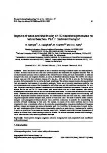
Because of all the uncertainties surrounding particle shape and the exact nature of grain-fluid interaction, Shields (1936) conducted a set of laboratory experiments to investigate how τ* would vary with the roughness Reynolds number (Re * = u*D/ν ).
0.06
The left hand, low-roughness-Reynolds-number part of the curve shows that fine grains, hidden partly within the laminar sublayer, would require a larger shear stress relative to their size than would somewhat larger, more exposed particles. This range is important in the quieter parts of large lowland rivers. For most rivers, we are concerned with the right-hand side of the graph, where Shields data roughly defines a dimensionless critical shear stress of 0.06. Hence the initiation of bed movement by turbulent open channel flow is traditionally evaluated using τc = 0.06 D g (ρs – ρ)
(14)
This relation was widely regarded as adequate for sand-bed rivers and little more was done until the late 1970s when application of (14) to gravel-bed rivers was thought to be inaccurate because the wider range of particle sizes on such beds causes a wider range of friction angles. Other complications due to particle shape, degrees of protrusion, and orientation were also thought to make Shields' value of 0.06 for τ* inappropriate for gravel-bed rivers.
3-10
Analyses of the case of non-uniform grain sizes have investigated the effect of changes in the friction angle and grain protrusion into the flow. The "cleanest" such studies tend to yield Shields-like results with the important difference that τ* is a strong function of grain size relative to the grains that compose the stream bed. Big particles can move over small particles at relatively low τc Small particles require a relatively higher τc to move them across beds of larger particles.
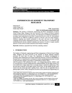
And, as an added complication, the % of sand in a mixed-sediment bed can profoundly alter the rate of sediment transport (see Wilcock et al., 2001, Experimental study of the transport of mixed sand and gravelWater Resources Research, 37(12):3349-3358—increasing sand content from 6 to 21% increased sediment transport by 1 to 3 orders of magnitude for the same water discharge!). Thus, it has proven surprisingly difficult to quantify the critical shear stress for motion of mixed-grain-size, coarse streambeds. Two methods of defining the initiation of motion have been commonly used: 1. Direct observations of the first movement as shear stress increases. This is notoriously difficult to do, even in a laboratory flume. 2. Measurement of bed load transport rates (qb) and plotting them against basal shear stress (τb). Extrapolation of the resulting trend to a value of qb = 0 has been the preferred method, either in the field or lab, but you can only use this for the average particle size.
τb
qb
3-11
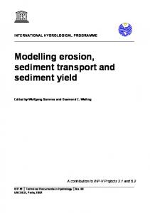
Empirically derived τ* values have distinct biases due to differences in experimental or observational methodology (Buffington and Montgomery, Water Resources Research, 1997): “Visual-based” (i.e. visually observed determination of first transport).
Oak Creek
“Reference-based” (i.e. project qb to condition of zero transport).
So what value of τ* do you use? In part, the range of plausible values should correspond to the range expressed in the graphs above for your particular application—is the problem one of “first motion”? Or is it that of net bed load transport? In the summary of Buffington and Montgomery (1997): “Our reanalysis of incipient motion data for bed surface material indicates that (1) much of the scatter in Shields curves is due to systematic biases that investigators should be aware of when choosing and comparing dimensionless critical shear stress values from the literature; and (2) there is no definitive τ*50 value for the rough, turbulent flow characteristic of gravel-bedded rivers, but rather there is a range of values that differs between investigative methodologies. Our analysis indicates that less emphasis should be placed on choosing a universal τ*50 value, while more emphasis should be placed on choosing defendable values for particular applications, given the observed methodological biases, uses of each approach, and systematic influences of sources of uncertainty associated with different methods and investigative conditions.”
3-12
Deposition / Settling Velocity of Particles in Still Water Transport of grains occurs when instantaneous vertical component of flow exceeds the settling velocity of particles.
Fall velocity in still water is influenced by two sets of forces: 1 submerged weight of particle 2 viscous fluid resistance and inertia effects Small and big particles behave differently: for small particles, viscous resistance dominates; inertia is negligible. for large particles that fall quickly, inertial forces dominate. Conditions under which of these effects dominates can be discerned using a particle Reynolds number (Rep) Rep = ω0 D / ν
(15)
where ω0 is the fall velocity, D is the particle diameter, and ν is the kinematic viscosity of the fluid. Based on experiments, inertia is negligible where Rep < 1: the boundary layer around the particle is laminar, and the fall is smooth (silt and clay). For Rep > 100, the viscous force is negligible, the boundary layer around the particle is turbulent, fall is rough, and a wake develops (gravel).
3-13
Stokes Law Stokes (1851) considered the problem of the balance between the downward force due to the submerged weight of a particle and a viscous resistance force and thereby got a "law" named after himself. Submerged weight of a spherical particle W = (π/6) D3 (ρs – ρ) g
(16)
Hopefully, this looks familiar [recall equation (2)]
Viscous resistance = f ( surface area, dynamic viscosity, and fall velocity ) V = 3 π D μ ω0
(17)
where μ = dynamic viscosity and ω0 = fall velocity.
Assuming no acceleration of a falling particle (i.e., constant terminal velocity, ωs) then W = V and (π/6) D3 (ρs – ρ) g = 3 π D μ ρs
(18)
Rearranging (18) in terms of the fall velocity yields ωs = (1/18) D2 (ρs – ρ) g / μ
(19)
Hence the fall velocity of small particles (i.e. with no inertial effects; see eqn. 17) is proportional to the square of the diameter. Note also that the settling velocity depends upon the viscosity of the fluid—colder temperatures or high sediment concentrations can make larger particles behave like finer ones and settle slower, thereby allowing smaller upward velocity fluctuations to keep them suspended above the stream bed. 3-14
Inertial Law Particles larger than about 2 mm (i.e., sand) encounter resistance from the "impact" force given by the momentum per unit time of the cylindrical column of water whose cross-section area is the projected area of the falling grain. The impact force is given by I = (1/4) π D2 ρ ωs2
(20)
The force balance between the submerged weight of this falling particle and the impact force is given by equating (16) and (20), at which time ωo = ωs, the terminal settling velocity: (π/6) D3 (ρs – ρ) g = (1/4) π D2 ρ ωs2
(21)
Rearranging terms yields:
ωs =
(ρ − ρ ) 2 Dg s 3 ρ
(22)
Hence, large grains fall at a rate proportional to the square root of their size, which leads to a strong size dependence to the fall velocity of particles in streamflow:
Whether particles of a particular size stay suspended in the flow or settle to the bed depends on the magnitude of upward turbulence. 3-15
Suspended Sediment Transport Although the morphology of many river beds is set by bed load transport, the majority of sediment moved by rivers travels as suspended load.
Significance of suspended load •
accounts for 80 - 95+% of sediment flux to oceans
•
flood plain formation: flux of sediment to flood plain = suspended load + overbank discharge
•
At low slopes and discharges, a suspended sediment layer can develop on stream beds and be incorporated into streambed gravels
•
Many water-quality contaminants travel as adsorbed constituents on the surface of suspended sediment particles—so water-quality problems commonly can be analyzed only by understanding the suspended-sediment transport
The total suspended sediment load is normally described as: z=H
Qsusp. =
∫ C(z) u(z) dz
(23)
z =0
where C(z) is the concentration profile of the suspended sediment.
What is the distribution of suspended sediment within the water column?
Particles settle via gravity to the bed at a terminal settling velocity, ωs. As particles settle, a concentration gradient develops, with more sediment deeper in the flow. However, the upward component of turbulence results in a mass flux up into the flow column that acts to maintain suspended sediment transport. The balance between downward settling and upward diffusion is what establishes the equilibrium concentration gradient and provides a means to develop a mathematical expression for that concentration.
3-16
Suspended Sediment Diffusion Two Processes 1
Settling by gravity occurs, with a terminal “settling velocity” of ωs. The downward flux of mass per unit area of a plane parallel to the bed is Fdown = Cωs
(24)
where C is the volumetric concentration of sediment (e.g., in units of kg/m3). This process concentrates sediment towards the bed of the channel.
2
Eddy exchange between layers in the turbulent flow causes a net flux of sediment between layers with a difference in sediment concentration—random turbulent interactions between layers cause intermixing at all levels, and therefore a net transport from areas of high concentration into areas of lower concentration. This net flux per unit area will tend to lift suspended sediment and is described by: Fup = –Ks (dC/dz)
(25)
where Ks is the “sediment mass diffusivity.” The negative sign results from flux down the concentration gradient (i.e. upward in the flow).
3-17
The sediment mass exchange by turbulence is a diffusion process (the flux is proportional to a potential gradient, in this case the concentration of suspended sediment). This process is analogous to the exchange of momentum that generates an eddy viscosity in the derivation of velocity profiles in turbulent flow (see the notes on the derivation of the “Law of the Wall”). In the case of momentum exchange, the flux of momentum per unit area of horizontal plane was the means by which a shear stress was exerted between layers. We first wrote that equation as τ = (μ + ε)(du/dz) (Equation 2-31), for which we then argued it could be adequately represented by τ = ε(du/dz). Here, we will define the eddy diffusivity as Km = ε/ρ, and so: τ = ρKm (du/dz)
(26)
where Km is the diffusivity of eddy momentum in the flow.
Vanoni made the analogy between the sediment mass diffusivity, Ks, and this corresponding water eddy momentum diffusivity, Km. He said that Ks ≈ β Km
(27)
where β should be less than 1 for coarser particles and converges on 1.0 for fine particles. In other words, β = 1 if the movement of sediment just tracks the movement of water, but larger particles can't keep up, so β < 1 for them.
(Please forgive the lack of any equations numbered “28” or “29”)
3-18
Recalling the derivation of the Law of the Wall, Prandtl argued that near the bed, τ ≈ τb (the shear stress on the bed) and that Km = k u* z. In this equation, k is Von Karman’s constant (0.4). With these assumptions, equation (26) can be re-written as: τ/ρ = Km (du/dz) = k u* z (du/dz)
(30)
Recall also from fluid mechanics that u* =
τb
ρ
or
τb / ρ =u*2
(31)
Substitution of equation (31) into equation (30) results in (du/dz) = u* / kz
(32)
Returning to equation (26) and by analogy to the Law of the Wall, at any level in the flow: τ /ρ = (τb /ρ) [(H – z)/H]
(33)
where H is the flow depth.
Combining (33) and (31) results in: τ /ρ = u*2 [(H – z)/H]
(34)
Substitution of equation (26) into the left hand side of equation (34) yields: Km(du/dz) = u*2 [(H – z)/H]
3-19
(35)
Similarly, substitution of equation (32) into equation (35) yields Km u*/kz = u*2 [(H – z)/H]
(36)
which can be rearranged to yield Km = u* kz [(H – z)/H]
(37)
This expression for the water eddy momentum diffusivity (Km), together with the assumption that Km ≈ Ks for fine particles (recall β ≈ 1.0), allows us to return to equation (25), the expression for the upward flux of suspended sediment due to turbulent diffusion:
Fup = –Ks(dC/dz)
(38)
= –βKm(dC/dz) = –β k z u* [(H – z)/H] (dC/dz)
Now we can consider the situation in which an equilibrium has been established between the two vertical sediment fluxes — (i) settling of particles and (ii) turbulent exchange of sediment mass. At this point (i) = (ii), Fup = Fdown, and C ωs = –β k z u* [(H – z)/H] (dC/dz) where C is varying with z; i.e., C = C(z).
3-20
(39)
To solve, we first separate variables in (39): dC / C = –[ωs /β k z u*] [H /(H– z)] dz
(40)
The solution of equation (40) is one of those for which the labor of finding does not enhance the utility of the result. So take it on faith (but check if you must) that: ln C = [ωs /β k u*] ln[H /(H– z)] + C’
(41)
where C’ is the constant of integration. If we choose the value of C’ cleverly, this equation can be rewritten as: ln C = ln Ca + [ωs /β k u*] ln{[H /(H– z)][a/(H – a)]}
(42)
where Ca is the concentration at some (any) one elevation above the bed at which z = a. Finally, this can be simplified as: a ⎤ ⎡H − z ⋅ C ( z) = Ca ⎢ H − a ⎥⎦ ⎣ z
ωs
u* k
(43)
assuming that β = 1. This more clearly expresses the form of the predicted relation for the concentration profile of suspended sediment as a power function of the distance from the bed surface. Note that in equation (43), the term a/(H–a) is less than 1 in the lower ½ of the flow (where, typically, any significant concentration of suspended sediment will be measured). The product with the term (H–z)/z is also less than one over most of the flow depth, and so raising it to an exponential power much greater than one will drive the value of C(z) towards zero. Thus the maximum value of the suspended sediment concentration will be determined by the empirically fit magnitude of Ca (and where in the flow that value was measured), but the rapidity with which that concentration gradient declines with distance away from the bed will be determined by the magnitude of the exponent, ωs/ku* —the larger this number (i.e. the coarser the sediment, or the lower the shear) the more abruptly will the concentration decline away from the bed.
3-21
This variable, ωs/ku*, is dimensionless (velocity ÷ velocity) and is known as the Rouse number (p = ωs/ku*).
In general, values of the Rouse number greater than about 2.5 lead to a condition of very little to no suspended sediment. In contrast, values of the Rouse number less than about 0.25 predict those grain sizes that will move as wash load, fully supported by the flow. In between these values lies the range of partial suspended sediment transport. A Rouse number less than 1.8 is sometimes suggested at an appropriate functional “threshold” for determining whether a given grain size will move in suspension (but note that the process itself is not threshold-driven!). Note also that smaller particles are predicted to be relatively evenly distributed through the flow column and that larger particles should be found only “close” to the bed. Although the form of equation (43) requires that the suspended sediment concentration be zero at the top of the water column (where z = H) regardless of particle size, we know from observations that this is not always the case. Which assumption(s) of the mathematical development is (are) not met in practice?
3-22
Ca in equation (43) can be estimated in three ways:
1. By fitting the equation to sediment concentration profiles measured with point samplers at various elevations above the bed.
2. By back-calculation from the vertically averaged sediment concentration measured in a depth-integrated suspended load sampler
3. By estimating the bed load flux (via equations or samplers), estimating the top of this bed load layer as a in (43), and converting the bed load flux through depth increment 0 0.2 mm in diameter, although the size of material that travels in suspension (suspended load) varies with the power and turbulence of the flow.
Bed load transport equations ignore the fact that grains move via turbulent bursts that must penetrate the laminar sub-layer, which shields grains from turbulence and movement of the flow. Because of this we back off from the force balance approach and develop relations between observed sediment transport rates and mean measures such as Q, S, W, h (or d), D50, or τb.
Each bed load transport formula has been developed and calibrated from specific conditions of τb S, D, and qb—so the basic rule of thumb is to use the one whose conditions best approximate your river.
Be smart about how you apply sediment transport equations—for example, if field evidence shows that transport only occurs in the middle of a river, then don’t use mean flow depth based on whole cross-section. Instead, use flow depth over the active transport zone or break the channel into zones with different flow depths. Attempts to calculate sediment transport are replete with cookbook application of formulas without any physical insight into the relevant conditions. Do the geomorphology first, and then try to attach some numbers to it!
3-25
Types of bed load transport (qb) equations Geologists and hydrologists have proposed numerous bed load transport equations; they fall into four general types:
1.
Excess Shear Stress [qb = f(τb – τc)]
2.
Stochastic (i.e. probabilistic)
3.
Stream Power [qb = f(Q, S) or f( Q/W, S)]
4.
Empirical Correlation
1. Excess Shear Stress Most bed load transport equations represent qb as the difference between the applied and critical parameters required for initiation of grain mobility: qb ∝ (τb’ – τc)β
(46)
where τb’ is the effective boundary shear stress (i.e. applied to the bed sediment), τc is the critical boundary shear stress required for grain movement, and β is an empirical exponent, typically > 1. a)
Du Boys (1879)
The oldest approach to excess shear stress: qb = φτb (τb – τo)
(47)
where φ = (0.173)/(D50)3/4 with D50 in mm, and τo is almost (but not exactly) Shield’s τc (which, recall, is a function of D50).
3-26
b)
Meyer-Peter equation
An empirical relation based on a large number of experiments with uniform sediment 3–29 mm, in flumes 20–200 cm wide, and depths < 20 cm. So: coarse sand, no bedforms, and grain roughness ≈ total roughness. The equation is traditionally (and somewhat confusingly) expressed in different units, depending on the system of measurement: For the SI system, the units of qb (sediment discharge) are kilograms of sediment transported per second per meter of channel width; q (water discharge) is in units of cubic meters per second per meter of channel width; and D50 (median sediment diameter) is in units of meters (not mm!). For the English system, the units of qb are pounds of sediment transported per second per foot of channel width (note that this is a unit of weight, not mass as for the SI version); q is in units of cubic feet per second per foot of channel width; and D50 (median sediment diameter) is in units of feet. The equation is: SI units:
English units:
qb = [250 q2/3 S – 42.5 D50]3/2
qb = [39.25 q2/3 S – 9.95 D50]3/2
(48a)
(48b)
Historically, the MP equation has been used to evaluate the bed load transport rate of different fractions of the bed load sediment population by substituting different values for D50 and multiplying the resulting qb by the fraction of total bed sediment represented by this size range. This is an effective way to investigate the routing of different sediment sizes down a channel. Unfortunately, such an approach has no theoretical justification and, in fact, has many reasons for why it is not correct. Such details have not stopped this practice!
3-27
c)
Meyer-Peter & Muller (1948)
An empirical relation based on a large number of experiments with uniform, graded, and lightweight materials; a more theoretically based expansion of the original Meyer-Peter equation. They formally suggested that a single effective grain diameter (D50) be used to characterize mixed sediment and that the total shear stress be modified to account for grain roughness, reducing the shear stress available for transporting sediment. Their empirical data were still flume-based but with a wider range of variables: grain sizes between 0.4 and 30 mm, depths between 1 and 120 cm, and a ratio of grain roughness to total roughness of 0.5 to 1. Their equation is: ⎡⎛ n ⎛ ρs ⎞ −1 ⎞ − ⎛ 2 ⎟⎟ ⋅ 8 ⋅ ⎜ ρ ⎟ ⎢⎜ grain roughness q b = ⎜⎜ ⎜ ⎝ ⎠ ⎢⎝ ntotal − roughness ⎝ ρs − ρ ⎠ ⎣
3 ⎤ ⎞ 2 ⎟ τ b − 0.047(ρ s − ρ )gD50 ⎥ ⎟ ⎥ ⎠ ⎦
3
2
(49)
qb is in units of weight per second per unit width of channel, and the entire equation is dimensionally homogeneous (so we don’t need to worry about which measurement system we are using—just be consistent!). Note that the last term in the brackets looks very much like Shield’s equation for τc with a slightly lower value for τ* (0.047 instead of 0.06). Note also that when this term exceeds the τb term, transport isn’t negative—it just doesn’t happen because the threshold of motion is presumed to have not yet been reached. ρs and ρ are densities of sediment and water (2650 and 1000 kg/m3), g is gravitational acceleration (9.81 m/s2). Grain and total roughnesses are represented with Manning’s n, where the grain roughness is defined by the Strickler (1923) equation: ngrain roughness = 0.0151 D501/6
(50)
where D50 is in mm, and ntotal roughness is determined by any of the methods normally used to estimate Manning’s n.
3-28
d)
Parker (1990)
Another empirical equation, based on analysis of data from Oak Creek, Oregon, a small paved gravel-bed channel. You will note that the equation does not specify a threshold for incipient sediment transport. Their analysis assumes subsurface sediment is the source of bed load, but this can occur only once the bed surface “pavement” is breached. Define first a dimensionless bed load transport rate, w*: ⎛ρ −ρ⎞ ⎟ qb ⎜⎜ s ρ ⎟⎠ ⎝ w* = 1 3 g 2 (dS ) 2
(51)
or, qb = g
1
2
3 ⎛ (dS ) 2 ⎜⎜ ρ
⎞ ⎟⎟ w* ⎝ ρs − ρ ⎠
(52)
Note that this is also dimensionally homogeneous, but that qb is in units of volume of sediment per second per unit width . Now the only problem is to determine w*. This is where the empirical data from Oak Creek came in: Parker expressed the data in two ranges, depending on the value of the dimensionless shear stress of the stream as expressed by yet another dimensionless parameter, φ50:
φ 50 =
where
τb ρgdS 0.0876 = 0.0876 (ρ s − ρ )gDspvt 50 (ρ s − ρ )gDspvt 50
(53)
Dspvt50 is the median diameter of the subpavement, not the surface sediment.
We can now solve Parker’s equation for qb by determining w*: w* = 0 w* = 0.0025 exp[14.2(φ50 – 1) – 9.28(φ50 – 1)2] w* = 13.69 [1 – (0.853/φ50)]4.5
3-29
for φ50 < 1 for 1 < φ50 < 1.6
(54a) (54b)
for 1.6 < φ50
(54c)
Stochastic Approach The Einstein (1950) bed load transport formula is the most complex procedure developed for natural streams.
It is a probabilistic approach, based on sand bed rivers in the Mississippi basin. He assumed that the number of particles eroded per unit time equals the number of particles on the bed times the probability of any one being eroded in an a unit time. We can consider sediment transport in 2 ways: the number of grains leaving a unit area in a unit period of time, and the number of grains entering an area in a unit period of time. The former (leaving grains) is expressed in terms of the probability of entrainment and the settling time of a grain once entrained (notice this assumes that saltation is the mode transport); the latter (entering grains) is expressed in terms of the bed load transport rate (what we will eventually want to solve for) and the length that a saltating grain will “hop.” At steady state, these two rates are equal. The probability of entrainment is a function of the lift forces and the buoyant weight of the particles. It has been determined by experiment and is expressed as a “flow-intensity index.” With corrections for grain hiding and hydraulic roughness, a “transport-intensity function” is read off a graph relating it to the corrected flow-intensity index and then converted into a bed load transport rate for the given particle size of interest. As with the Meyer-Peter equation, this equation is commonly run for discrete grain sizes under the assumption that each moves independently of the others. Insofar as this is a saltating system, presumably without a pavement layer, this assumption may not be as ill-conceived as in gravelbed systems.
3-30
Stream Power Approach Bagnold (1960, 1966) developed an approach to bed load transport prediction that is based on stream power per unit channel width (ω), which is defined as: ω = ρg (Q/w) S
(55)
He argued, reasonably, that ω was an appropriate measure of transport. Recall, from classical mechanics, that Work = force x distance Power = work/unit time = force x distance/time = force x velocity And because stress = force/area, Power/area (Bagnold’s ω, the unit stream power) = stress x velocity He also defined the power of the moving sediment per unit bed area as: (ρs – ρ)g (Vseds / Vbed) tan φ ⋅ useds where Vseds / Vbed is the concentration (by volume, V) of sediments on the bed. The entire first term of this expression looks very much like the frictional strength part of the slope-stability equation of classical landslide mechanics with φ, Bagnold’s “slipping angle,” playing the role of an angle of internal friction. Bagnold’s key assumption is that stream power is transmitted to moving sediment via an “efficiency factor, eb, that ranges from 0 to 100%. With a value of 0 there is no sediment motion; at 100%, there would be no dissipation of energy in the system at all except from the movement of grains (which is obviously impossible). USGS Professional Paper 422H tabulates presumed eb values as a function of mean water velocity. The method as a whole has never seen much application except in the analysis of very sedimentrich flows (such as debris flows).
3-31
Empirical Correlations Bagnold was convinced that stream power was the correct theoretical approach to the problem of sediment transport, but assessing the efficiency factor was very problematic and the focus of many subsequent papers. After nearly 2 decades, Bagnold gave up. Instead, he decided that even if an analytic form could not be defined, there surely were enough data to find an empirical relationship between unit stream power and sediment transport. In recognition of other potentially influential factors, he also included flow depth and grain size of the bed load in his final correlation. His equation was expressed in terms of “reference” conditions (marked with an asterisk, and so given values) and the subject conditions (unasterisked, user-supplied). The three terms of the equation are for “excess” unit stream power, flow depth, and modal grain size (normally, median can be substituted here). The equation is: 3
⎡ ω − ωo ⎤ 2 ⎡ Y ⎤ ib = ib* ⎢ ⎥ ⎢ ⎥ ⎣ (ω − ω o )* ⎦ ⎣ Y* ⎦
−2
3
⎡D⎤ ⎢ ⎥ ⎣ D* ⎦
−1
2
(56)
ib is in units of (watch closely!) the submerged mass rate of sediment transport per unit width of channel. To convert to dry mass, multiply by [ρs/(ρs-ρ)], or about 1.6. To convert to weight, multiply by g (i.e. 9.8 m/sec2 in SI units). Reference (i.e. *) values are as follows: ib* = 0.1 kg/m-sec (ω - ωo)* = 0.5 kg/m-sec Y* = 0.1 m D* = 1.1 x 10⁻³ m (about 1 mm, but remember that the units are METERS!) For “your” stream, Y = average flow depth and D = modal grain size (both in m). ω is the unit stream power, calculated from the definition (equation (55) above). ωo is the unit stream power at the threshold of motion; Bagnold assumed a Shields parameter of 0.04 and substituted that into the definition of ω as the product of shear stress and mean velocity to get: ωo = 290 D1.5 log[12Y/D]
3-32
(57)
Summary and Comparison of Bed Load Transport Equations Each equation has a particular range of “best” applicability, a function of both the assumptions and the size of the sediments and flow conditions used to extract the empirical coefficients (a.k.a. “fudge factors”). In particular, those with explicit data sets have an obvious established range; Bagnold’s original stream-power approach required very concentrated flows to work well, and the stochastic approach requires abundant saltating grains (i.e. sand) and good measurements.
Accuracy is a tremendous problem with these equations. Methods may vary by an order of magnitude (or more) in their predictions. Sometimes as good an estimate can be made by assessing the basin sediment yield and assuming that 1-10 percent of that will travel as bed load. Also beware of supply-limited systems, which violate assumptions of these methods.
See: Gomez and Church, Wat. Res. Research, v. 25(6), p. 1161-1186 Most sediment transport formulae characteristically overpredict sediment flux by 2-10 times due to: • failure to include surface coarsening • variations in the rate at which material is supplied and available for transport Best equations in general appear to be Bagnold (for gravel-bed rivers) and Einstein (for sand-bed rivers). Parker equation is a great favorite among theoretical geomorphologists and is good most of the time, but at other times gives really wacky answers
3-33
So, how to approach a sediment routing calculation? 1.
Sediment Supply • •
• 2.
Is bed material bed load or suspended load? Is there another source of bed load that moves over an immobile substrate? Need to determine source and texture of sediment for your problem
Scales of bed load movement • •
3.
Bankfull bed load movement Low-flow fine sediment movement
Bed armoring •
4.
pavement or no pavement
Which formula to use? • Consult Gomez and Church for equation that best fits your channel.
5.
Hydraulic parameters (u, H, S, & D) •
How do you get these values and are they realistic?
•
Where do you sample D in a channel?
•
Choose the obviously mobile patches and the most representative.
•
Do calculations for simple, straight, plane-bed reach if possible as you can get a valid average flow depth (H).
•
Don’t always cross-section average - i.e., don’t use average depth in a non-rectangular channel.
3-34
Flow in Bends The radius of curvature Definition: the radius of the arc that traces out the meander path (not really circular, but that’s ok). By observation, many rivers have a ratio rc/w = 2 or 3; studies of channel migration rates suggest that rivers migrate more rapidly as this ratio increases (i.e. straight rivers migrate fastest). Why is this? Studies on pipe flow suggested that frictional resistance was lowest in this range; other flume studies note that at radii much different from this range, either the upstream limb migrates more rapidly than the downstream limb (too large) or visa versa (too small). Either way, the result is convergence on this range—so it’s not that the river somehow “prefers” this curvature, it’s just that other curvatures are less stable on the landscape.
c
3-35
Superelevation The centrifugal force of the water accelerating around the bend must be balanced by something (or else it would continue to climb ever-higher)—it’s the cross-stream pressure gradient imparted by the superelevation (Δh):
ρu 2 h rc
= ρgh
Δh w
(58)
u2w rc g
(59)
And so: Δh =
Note the typical scale of the superelevation: rc / w is about 2 or 3; for a river with a flow of about 1 m/s, Δh is a few cm. The pressure gradient balances the average flow velocity, but near the surface the local velocity exceeds the average velocity and so the centrifugal force exceeds the pressure; at depth, average velocity exceeds the local velocity and so the pressure exceeds the centrifugal force:
So bottom flow is towards the inside of the bend. This is secondary flow (“primary flow” is in the downstream direction).
3-36
3-37
Consequences for sediment transport First, note the basic conditions that establish the spatial patterns of sediment erosion and deposition: • • •
Erosion occurs where τb is increasing in the downstream direction. Deposition occurs where τb is decreasing in the downstream direction. You won’t find grains of a particular size unless they can be transported to their point of deposition. So, in general, you will find the coarsest bed particles along the path of τmax (or where τmax was when the channel was at a sediment-transporting stage!).
In addition, bedforms tend to channelize the secondary flow (because it moves along the bed), and so the idealized pattern can be modified by the sedimentary deposition that results from it: the flow shapes the bed, but the bed alters the flow. Any such system presents opportunities for both negative feedback (i.e. stable channel form) and positive feedback (i.e. rapid instability and migration).
3-38