Linear Combinations of Heuristics for Examination Timetabling Edmund K. Burke*, Nam Pham*, Rong Qu*, Jay Yellen*†
*
ASAP Group, School of Computer Science
University of Nottingham, Nottingham, NG8 1BB, UK. {ekb|nxp|rxq}@cs.nott.ac.uk
†
Department of Mathematics and Computer Science, Rollins College
Winter Park, Florida, 32789, USA
[email protected]
Abstract: Although they are simple techniques from the early days of timetabling research, graph colouring heuristics are still attracting significant research interest in the timetabling research community. These heuristics involve simple ordering strategies to first select and colour those vertices that are most likely to cause trouble if deferred until later. Most of this work used a single heuristic to measure the difficulty of a vertex. Relatively less attention has been paid to select an appropriate colour for the selected vertex. Some recent work has demonstrated the superiority of combining a number of different heuristics for vertex and colour selection. In this paper, we explore this direction and introduce a new strategy of using linear combinations of heuristics for weighted graphs which model the timetabling problems under consideration. The weights of the heuristic combinations define specific roles that each simple heuristic contributes to the process of ordering vertices. We include specific explanations for the design of our strategy and present the experimental results on a set of benchmark real world examination timetabling problem instances. New best results for several instances have been obtained using this method when compared with other constructive methods applied to this benchmark dataset.
Keywords: examination timetabling, weighted graph, constructive heuristics, heuristic combinations, graph colouring heuristics
1 Introduction The university examination timetabling problem consists of assigning each exam to a timeslot subject to various practical constraints. There are both hard and soft constraints in examination timetabling. Hard constraints must be satisfied in a strict manner. Timetabling solutions that cause hard constraint violations (infeasible solutions) are typically considered to be significantly inferior to 1
solutions that do not. Soft constraints express a preference among feasible solutions. Designing timetables that satisfy various constraints presents a challenging task particularly for large educational institutions with hundreds or thousands of exams and students. That challenge motivated many research efforts to exploit the computing power of computers to construct timetables for a large set of exams rather than doing so manually (Bardadym 1996). One of the most popular early approaches, graph colouring heuristics, in the exam timetabling research literature is based on graph colouring models. A graph colouring problem involves the assignment of a limited set of colours to vertices such that adjacent vertices receive different colours (non-conflict). For exam timetabling problems, exams to be scheduled can thus be represented by vertices, and timeslots are represented by colours in the graph colouring model. Two vertices connected by an edge (i.e., adjacent vertices) represent the corresponding exams having at least one student in common, and thus they must not be assigned the same colour (timeslot). The weight of an edge between two vertices represents the number of students taking both corresponding exams. Conflict-free colourings represent timetables that satisfy the hard constraint. The exam timetabling problem differs from the traditional graph colouring problem in the objective function. Classical graph colouring focuses on minimizing the number of colours needed to construct a feasible colouring (achieving the chromatic number). Whereas for exam timetabling, the goal is to find a feasible colouring that uses a pre-specified number of colours while maximizing the satisfaction of additional soft constraints. For example, one of the most common soft constraints is to spread examinations in the timetable for students. This is typically evaluated by the sum of penalties incurred by assigning adjacent exams to timeslots too close to each other. Given that graph colouring is NP-Hard (Papadimitriou and Steiglitz 1982), significant research has been devoted to the design of constructive approximate algorithms, which sacrifice the guarantee of optimality but produce solutions in a reasonable amount of computation time. The graph colouring algorithms involve two simple steps: vertex selection and colour selection. The strategy behind vertex selection is based on the idea that we should colour the most troublesome or difficult vertices as early as possible. Here, a troublesome or difficult vertex is one that is most likely to lead to a poor or infeasible timetable if its colouring is deferred until later in the process. A logical heuristic for the colour assignment for a vertex is that it should incur the lowest penalty in the objective function and also cause least trouble for the vertex’s uncoloured neighbours. Much of the research on constructive algorithms has focused on the vertexselection heuristics. The most popular ones include saturation degree (Brelaz 1979) and largest (weighted) uncoloured degree. Carrington et al. (2007) introduced an enhanced weighted graph model extending the weighted graph model first proposed by Kiaer and Yellen (1992). In the enhanced weighted graph model, each edge and vertex keeps track of more information relevant to the objectives than in the traditional graph model. As a result, several new vertex- and colour-selection heuristics emerged and showed promising results in their use within the approximate algorithm (Carrington et al. 2007). In many decision-making scenarios, it is often better to take into account several factors simultaneously than to rely on only one factor. For instance, Asmuni et al. (2005) used a fuzzy inference system for course timetabling to 2
combine three heuristics to identify the difficult vertices, and the results appeared to be superior to using any single heuristic. Motivated by that, we extended our previous weighted graph model (Carrington et al. 2007) and propose in this paper a new strategy of using linear combinations of several primitive heuristics for vertex selection. Each heuristic in the combination is weighted according to its effectiveness on different weighted graphs. This strategy provides very competitive results compared to other constructive methods in the literature for several of the Toronto benchmark exam timetabling instances (Carter et al. 1996; Qu et al. 2009). Although there is still a gap between the results obtained in this paper and the best results reported in the literature using advanced improvement based techniques, this work represents a step towards more effective integration of simple heuristics for constructing timetables. We focus on providing a bridge for future work, and several research directions emerge based on the approach investigated here. This paper is organised as follows. Section 2 reviews related approaches and techniques for exam timetabling problems in the literature and describes the widely studied Toronto problem instances on which our model is tested. We then review the enhanced weighted graph model in Section 3. In Section 4, we define a new strategy using linear combinations of heuristics and justify through experiments our decisions regarding various features of these linear combinations. Experiments in Section 5 demonstrate the effectiveness of the linear combination approach in comparison with the best reported solutions obtained from other constructive approaches. We test our approach with and without vertex partitioning, which was introduced in Carrington et al. (2007). By comparing the results of our approach to another constructive approach, we show that integrating our linear-combination strategy with other techniques (e.g. backtracking) can improve on the current performance and represents a promising research direction. Section 6 provides conclusions and summarises future research directions.
2 Exam Timetabling Problems Graph colouring approaches to timetabling have been studied since the 1960s (e.g. Broder 1964; Welsh and Powell 1967; Wood 1968; Neufeld and Tartar 1974; Brelaz 1979; Mehta 1981; Krarup and de Werra 1982). Several surveys have reviewed work on this topic (e.g. Schmidt and Strohlein 1980; de Werra 1985; Carter 1986; Schaerf 1999; Burke et al. 2004; Qu et al. 2009). As simple and fast techniques, graph heuristics in timetabling had many advantages, particularly when being used in the initialisation process for meta-heuristics, or integrated with meta-heuristics in various ways (e.g. Burke et al. 2004; Merlot et al. 2003). Another early methodology in timetabling is constraint based methods (e.g. Banks et al. 1998; Nonobe et al. 1998), sometimes hybridised with meta-heuristics (Merlot et al. 2003). Meta-heuristic techniques (e.g. Glover et al. 2003; Reeves 1996) have attracted significant research interest and became the state of the art through their success on various complex timetabling problems. Such techniques include Tabu Search (e.g. Di Gaspero et al. 2000), Simulated Annealing (e.g. Dowsland 1998; Abramson et al. 1999) and Evolutionary Algorithms (e.g. Burke and Newall 1999; Terashima-Marin et al. 1999). 3
More recent research includes Ant Algorithms (e.g. Socha et al. 2002), CaseBased Reasoning (e.g. Burke et al. 2006), fuzzy reasoning (e.g. Asmuni et al. 2005), GRASP (e.g. Casey et al. 2002), Very Large Scale Neighbourhood Search (e.g. Abdullah et al. 2007), Variable Neighbourhood Search (Qu and Burke 2005) and Hyper-heuristics (e.g. Burke et al. 2003). A number of survey papers also appear that overview the timetabling literature (Bardadym 1996; Burke et al. 2004; Carter et al. 1996; Carter et al. 1998; Petrovic et al. 2004; Reeves 1993; Schaerf 1999). In this paper we focus on one of the most widely tested sets of problem instances in the timetabling research community -- the Toronto benchmark examination timetabling problems (Carter et al. 1996; Qu et al. 2009) (publicly available at ftp://ftp.mie.utoronto.ca/pub/carter/testprob/). This dataset has been the benchmark since its introduction in 1996, and still remains an interesting challenge to the research community. Therefore, we test our method on this benchmark and compare our results against many other existing methodologies applied on the same dataset. The optimal solutions for all instances in this dataset have not been found yet. During the years, researchers are reporting the best results obtained along with the development of advanced algorithms. Table 1 shows characteristics of the 12 instances. Table 1 Details of the Toronto exam timetabling benchmark (Carter et al. 1996; Qu et al. 2009) Instances car91 I car92 I ear83 I hec92 I kfu93 I lse91 rye92 sta83 I tre92 uta92 I ute92 yor83 I
No. of Exams 682 543 190 81 461 381 482 139 261 622 184 181
No. of Students 16925 18419 1125 2823 5349 2726 11483 611 4360 21266 2749 941
Enrolments 56877 55522 8109 10632 25113 10918 45051 5751 14901 58979 11793 6034
Density 0.13 0.14 0.27 0.42 0.06 0.06 0.07 0.14 0.18 0.13 0.08 0.29
Timeslots 35 32 24 18 20 18 23 13 23 35 10 21
Two versions of the dataset have circulated under the same name over the last ten years. We used the naming convention provided in (Qu et al. 2009). One of the 13 instances in the dataset, pur93, is excluded due to the inconsistency in the data file over different versions. Qu et al. (2009) provided an extensive survey on all search methodologies with associated best reported results for this dataset.
3 The Enhanced Weighted Graph Model Our current work builds upon the model introduced in Carrington et al. (2007). The enhanced model incorporates considerably more information that is continually updated as the colouring progresses. This readily available information led to the design of several new vertex-selection heuristics, some of which are generalisations of traditional heuristics such as saturation degree and 4
largest (weighted) degree. We also introduced ‘badness’ thresholds by which certain colours are considered bad for a given vertex or only certain bad edges are counted toward the vertex’s degree or weighted degree.
Basic model features and parameters
Our primitive vertex-selection heuristics are based on the following list of basic features and parameters: Intersection size (of an edge e) - simply the number of students taking both exams. Intersect degree (of a vertex) - the sum of the intersection sizes of edges adjacent to the vertex. Average intersection size - the average of the intersection sizes of all edges in a graph. Bad-intersect edge - an edge whose intersection size exceeds a specified threshold Te = averageIntersectionSize * ie, where ie is a multiplier parameter. Conflict – incurred when the same colour is assigned to the two adjacent vertices of an edge. Conflict penalty (for the colour assignment of a vertex) - indicates the number of conflicts incurred with all neighbours of that vertex from the colour assignment. Proximity (of two colours ci and cj) - a measure of how close together the two colours are. For the Toronto instances, the timeslots are simply ci = i, i = 0,1,.... If 0 < | i – j | ≤ 5, the two colours are close together or ‘in proximity’. Proximity penalty (for assigning two colours ci and cj to the adjacent vertices of an edge e) – equals the product 25-|i-j| * intersectionSize(e) if the two colours are in proximity and 0 otherwise. The first part of the product 25-|i-j| is the proximity weight for the Toronto instances. Proximity penalty (for the colour assignment of a vertex) - the sum of the proximity penalties resulting from that colour assignment and the colour assignments of all neighbours of that vertex. Colour-penalties vector (of a vertex) - indicates for each colour the conflict penalty and proximity penalty of assigning that colour to the vertex. When a vertex is coloured, the colour-penalties vector of each of that vertex’s neighbours must be updated accordingly. Bad-conflict colour (for a vertex) - a colour whose conflict penalty for that vertex differs from 0; for the Toronto instances, zero conflict penalty is required. Bad-proximity colour (for a vertex) - a colour whose proximity penalty for that vertex exceeds some specified threshold Tc = averageIntersectionSize * ev * pc, where ev is the expected value of the proximity weight and pc is a multiplier parameter (see Appendix A for a derivation of ev and an explanation of its use). Bad colour (for a vertex) - either a bad-conflict colour or a bad-proximity colour for that vertex. Primitive heuristics
Each primitive vertex-selection heuristic represents a different measure of how troublesome a vertex is. The following list contains the seven primitive vertexselection heuristics used in this paper. 0. 1. 2. 3.
Number of bad colours. Number of bad-conflict colours (saturation degree). Number of bad-proximity colours. Sum of the proximity penalties. 5
4. Number of edges to uncoloured neighbours (largest uncoloured degree). 5. Number of bad-intersect edges to uncoloured neighbours. 6. Intersect degree to uncoloured neighbours (weighted uncoloured degree).
The four primitive heuristics used to select a colour for a given vertex are: 0. Minimum conflict penalty. 1. Minimum proximity penalty. 2. Minimum number of good-to-bad conflict colour switches for the uncoloured neighbours. 3. Minimum number of good-to-bad proximity colour switches for the uncoloured neighbours.
Advanced model features
In addition to the new primitive heuristics, the enhanced model enables us to combine any number of primitive heuristics to form compound vertex or colour selectors. A compound selector applies the primitive heuristics in a sequence to narrow down the list of selected vertices or colours. All but the first heuristic in a sequence act as tiebreakers for the preceding ones provided that the list is still greater than one. The compound selector is at least as effective in identifying an appropriate vertex or colour as a selector based on a single criterion. The model also allowed a compound selector to switch to another compound selector at the middle of a colouring process. This feature was motivated by the observation that the effectiveness of a heuristic is likely to change as the colouring progresses. For instance, the saturation degree heuristic is not an effective predictor of troublesome vertices in the early stages of a colouring, when the vertices are mostly all unsaturated, i.e., they all have almost no forbidden colours and the same number of valid colours. In the implementation, there was one ‘switching point’ typically set at an early stage after a certain number of vertices had been selected and coloured using some other non-saturation-degree-based selector. The final feature of the model - vertex partitioning - is a pre-processing step. First, the set S1 of vertices with degree less than the number of available colours in the original graph are designated easiest and assigned colours only after all other vertices have been coloured. These vertices can be coloured last, since each of them will always have at least one non-conflict colour available. The same procedure can be applied to the reduced graph formed by deleting the vertices in S1 (and their adjacent edges), resulting in the next easiest vertex subset S2. The process continues until there are no more easy vertices left. We refer to the remaining subset of vertices as the hardest vertex subset. The colouring process reverses this partitioning order, i.e. the hardest vertex subset is coloured first and the easiest vertex subset S1 is coloured last. The potential advantage of this vertex partitioning feature is that vertex-selection process for easy subsets can be based solely on proximity. The following groups of compound vertex and colour selectors used in our previous work illustrate the use of these advanced model features. We designed two groups of three compound vertex selectors: 6
vs1: 4 5 6 1 2 3 | 1 4 2 3 5 6 | 2 3 5 6 vs2: 4 5 6 0 3 | 0 4 5 6 2 3 | 2 3 5 6
and two groups of two compound colour selectors: cs1: 0 1 2 3 | 0 1 3 cs2: 0 2 3 1 | 0 3 1
The numbers in these groups refer to the indices of the primitive heuristics. The vertical lines separate different compound selectors. We used the vertex partitioning in all experiments in the previous work, and the last compound selector was always applied to all the easy vertex subsets. The first compound vertex selector was applied to the hardest vertex subset until a specified fraction (the switching point) of the vertices had been coloured. Then the second compound vertex selector was applied for the rest of the hardest vertex subset. The first compound colour selector was applied to the entire hardest subset, and the second selector was then applied to all other subsets.
4 Linear Combinations of Primitive Vertex-Selection Heuristics The selector strategy in our previous work used sequences of primitives as tiebreakers to form compound vertex selectors. However, in a recent experiment, we observed that many tiebreakers in the sequence were often unnecessary because the set of candidates had been narrowed down to a single vertex. The experiment examined the performance of the compound vertex selector vs1 (listed above) with a particular set of parameters (pc=50, ie=2, switchingPoint=1), and compound colour selector: cs1 applied to the hardest vertex subset of the 12 Toronto problem instances. Table 2 shows the number of times the set of the most troublesome vertices was narrowed down to one vertex after applying a particular heuristic in the sequence. On the majority of occasions, this happened after only the first two heuristics were used. As a result, the remaining primitive heuristics in the sequence played no role in the vertex selection. The problem instance sta83 I was unique in that there were 32 times in which the set of troublesome vertices was not narrowed down to one vertex after applying six primitive heuristics in the sequence. Table 2 The depth level of primitive heuristics called for the hardest vertex subset using vs1. Values in parentheses denote the size of the hardest vertex subsets
Primitive 4 Primitive 5 Primitive 6 Primitive 1 Primitive 2 Primitive 3 Unnarrowed
car91 I (507)
car92 I (392)
ear83 I (157)
hec92 I (70)
kfu93 I (196)
lse91
rye92
tre92
(189)
sta83 I (78)
(124)
112 341 38 16 0 0 0
102 259 18 13 0 0 0
40 103 6 8 0 0 0
30 32 2 6 0 0 0
66 117 2 11 0 0 0
33 85 1 5 0 0 0
ute92
(193)
uta92 I (458)
(89)
yor83 I (176)
74 102 3 10 0 0 0
11 22 0 13 0 0 32
44 132 5 12 0 0 0
95 296 38 29 0 0 0
30 52 2 5 0 0 0
46 117 4 9 0 0 0
7
This observation motivated a new strategy that combines primitive heuristics more effectively. The compound vertex selectors are now (weighted) linear combinations of the primitive vertex-selection heuristics. To identify the most troublesome vertices, we apply a heuristic evaluation function f to each of the uncoloured vertices, and a vertex having the largest evaluation value is chosen. In the current implementation, our function f is a linear combination of seven characteristics (parameters) tied to the partial colouring of the weighted graph. In particular, for each uncoloured vertex v, f (v )
a o xo
a1 x1
... a6 x6 ,
(1)
where ai are nonnegative weights and x0 = number of bad colours counted from the colour-penalties vector of v. x1 = number of bad-conflict colours counted from the colour-penalties vector of v. x2 = number of bad-proximity colours counted from the colour-penalties vector of v. x3 = sum of the proximity penalties over all colours stored in the colour-penalties vector of v. x4 = number of edges to v’s uncoloured neighbours. x5 = number of bad-intersect edges to v’s uncoloured neighbours. x6 = intersect degree to v’s uncoloured neighbours.
This linear-combination approach is adaptable to colour selection as well, although in this paper, we focus only on the vertex-selection process.
Heuristic selections and weight settings for linear combinations
The main task in designing linear combinations of primitive heuristics is to decide how the weight vector [a0, a1, ..., a6] is to be set. We describe our approach here and justify our decisions by experiments on the 12 Toronto benchmark instances. In these experiments, we use the vertex partitioning step described earlier. The compound colour selector cs1: 0 1 2 3 | 0 1 3 from our previous work is applied (Carrington et al., 2007). The multiplier parameters for the bad-proximity colour threshold and the bad-intersect edge threshold were varied as follows: pc = 5 to 75 in increments of 2 ie = 0.5 to 5 in increments of 0.5 The results obtained from the algorithm give the average proximity penalty over all students. Because our approach is based on a constructive algorithm, the results obtained in this paper will be compared to the best results from other constructive methods, shown in the first four columns in Table 3 (and marked with a †). Also, for the purposes of comparison, the last four columns in the table show the current best results of non-constructive approaches involving iterative improvement. All of these results were drawn from the survey paper by Qu et al. (2009). Note that the aim of this work is to explore effective integrations of simple constructive heuristics in timetabling research, rather than to ‘beat’ the best results from complicated meta-heuristics. Both of these are directions of current research in timetabling. Comparisons between constructive approaches and complicated meta-heuristics provide little insight in the context of this study. Nevertheless, we 8
do list in Table 3 the results of both types of approaches to give an overall view of the current achievement on this benchmark. Table 3 A comparison of results obtained using different approaches. Constructive approaches are marked with a dagger (†). The last four columns show the best approaches involving iterative improvement techniques. Bold font indicates the best results achieved by any method; underlined text indicates the best results obtained by a constructive method Problem
car91 I car92 I ear83 I hec92 I kfu93 I lse91 rye92 sta83 I tre92 uta92 I ute92 yor83 I
†(Carter †(Burke †(Asmuni †(Burke (Caramia (Cote et al. 1996)
et al. 2004)
et al. 2005)
et al. 2006)
et al. 2001)
et al. 2005)
7.1 6.2 36.4 10.8 14.0 10.5 7.3 161.5 9.6 3.5 25.8 41.7
5.0 4.3 36.2 11.6 15.0 11.0 161.9 8.4 3.4 27.4 40.8
5.29 4.56 37.02 11.78 15.81 12.09 10.35 160.42 8.67 3.57 27.78 40.66
5.36 4.53 37.92 12.25 15.2 11.33 158.19 8.92 3.88 28.01 41.37
6.6 6.0 29.3 9.2 13.8 9.6 6.8 158.2 9.4 3.5 24.4 36.2
5.4 4.2 34.2 10.4 14.3 11.3 8.8 157.0 8.6 3.5 25.3 36.4
(Yang
(Burke
& Petrovic 2005) 4.5 3.93 33.7 10.83 13.82 10.35 8.53 158.35 7.92 3.14 25.39 36.35
et al. 2010) 4.6 4.0 32.8 10.0 13.0 10.0 159.9 7.9 3.2 24.8 37.28
The effectiveness of using heuristic x0 – number of bad colours
The first four of the seven primitive vertex-selection heuristics, repeated below, are based on the information retained in the vertices’ colour-penalties vectors. Accordingly, we classify them as colour-penalties-based vertex-selection heuristics. x0 = number of bad colours counted from the colour-penalties vector of v. x1 = number of bad-conflict colours counted from the colour-penalties vector of v. x2 = number of bad-proximity colours counted from the colour-penalties vector of v. x3 = sum of the proximity penalties over all colours stored in the colour-penalties vector of v.
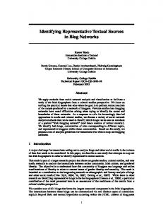
In this group, we claim that heuristic x0 should play a role in linear combinations because it is essentially a consolidation of heuristics x1 and x2. Heuristic x2 is analogous to saturation degree (x1) but is based on proximity instead of conflict. In our previous work, we also claimed that heuristic x2 may be better at evaluating the trouble level of a vertex than its sum counterpart, heuristic x3. An extreme example in Figure 1 shows the colour-penalties vectors of two vertices v1 and v2. Suppose that there are four available colours for each vertex (represented by the four component-pairs in each colour-penalties vector), the first value in each component represents the conflict penalty and the second represents the proximity penalty. If we set a bad-proximity-colour threshold 0 ≤ Tc < 50, heuristic x2 would return four bad-proximity colours (underlined in Figure 1a) from v1’s evaluation and as a result, favour v1 over vertex v2, which has only one bad-proximity colour (underlined in Figure 1b). On the other hand, heuristic x3 always selects vertex v2 with the proximity penalty sum of 201 before v1 whose proximity penalty sum equals 200. 9
Fig. 1 Colour-penalties vectors of an example where heuristic x2 is probably better than heuristic x3. Heuristic x2 would select vertex v1 and heuristic x3 would select vertex v2, if the badproximity-colour threshold 0 ≤ Tc < 50
The experimental results shown in Table 4 below reinforce these claims. The experiment used the following groups of linear combinations: vs1: x0 | x2 vs2: x1 | x2 vs3: x2 | x2 vs4: x3 | x2 vs5: x1 + .00001x2 | x2 vs6: x1 + .00001x3 | x2
The vertex selector to the left of the vertical line is applied to the hardest vertex subset (first), and the one to the right is then applied to all the easy subsets. Vs5 and vs6 can be understood as compound selectors because we set a small enough weight (.00001) so that heuristics x2 and x3 act as tiebreakers for x1, respectively. For the easy subsets, we always choose heuristic x2 to select the most troublesome vertices since it concerns only proximity and is favoured over its sum counterpart x3. The results suggest the superiority of heuristic x0 over the three other primitives. Table 4 Comparisons on different groups of linear combinations of coloured-penalties-based heuristics. Bold font indicates the best results obtained among the linear combinations Problem car91 I car92 I ear83 I hec92 I kfu93 I lse91 rye92 sta83 I tre92 uta92 I ute92 yor83 I
vs1
vs2
vs3
vs4
vs5
vs6
5.23 4.47 38.05 12.28 infeasible 12.23 10.6 168.63 8.68 3.45 29.39 infeasible
5.44 4.85 44.1 infeasible infeasible 12.81 11.51 164.94 9.89 3.75 32.75 infeasible
infeasible infeasible infeasible infeasible infeasible infeasible infeasible infeasible infeasible infeasible infeasible infeasible
infeasible infeasible infeasible infeasible infeasible infeasible infeasible infeasible infeasible infeasible infeasible infeasible
5.34 4.66 38.99 12.69 18.68 12.91 11.02 163.04 9.52 3.55 30.21 42.2
5.34 4.66 39.88 13.82 infeasible 13.33 11.49 165.11 9.14 3.6 31.2 infeasible
Best reported 5.0 4.3 36.2 10.8 14.0 10.5 7.3 158.19 8.4 3.4 25.8 40.66
10
Linear combinations of heuristics x0 and x5
The remaining three primitive vertex-selection heuristics are classified as edgebased vertex-selection heuristics since they are based on the (static) information retained in each vertex‘s adjacent edges to determine its difficulty. x4 = number of edges to uncoloured neighbours (uncoloured degree). x5 = number of bad-intersect edges to uncoloured neighbours. x6 = intersect degree to uncoloured neighbours (weighted uncoloured degree).
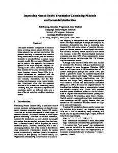
For the Toronto instances, heuristics x4 and x6 represent the traditional largest uncoloured degree and largest weighted degree respectively. We introduced heuristic x5 in our previous work that involves a threshold to determine when an intersection size of an edge is considered ‘bad’. We claimed that counting badintersect edges of a vertex may be better at evaluating the difficulty of the vertex than adding up all the intersection sizes of the incident edges (as done by heuristic x6). The example shown in Figure 2 illustrates this claim.
Fig. 2 Vertex-selection strategies for edge-based primitive heuristics x4, x5, x6. Heuristic x4 would select vertex v1, heuristic x6 would select vertex v3, and heuristic x5 would select heuristic v2 if the bad-intersect-edge threshold 1 ≤ Te < 50
Table 5 Comparisons on different groups of linear combinations between colour-penalties-based and edge-based vertex-selection heuristics. Bold font indicates the best results obtained among the linear combinations Problem car91 I car92 I ear83 I hec92 I kfu93 I lse91 rye92 sta83 I tre92 uta92 I ute92 yor83 I
vs1 5.23 4.47 38.05 12.28 infeasible 12.23 10.6 168.63 8.68 3.45 29.39 infeasible
vs2 5.21 4.29 37.65 12.52 16.93 11.46 9.83 160.26 8.57 3.47 28.41 41.1
vs3 5.19 4.39 38.71 12.38 18.21 11.49 10.04 162.6 8.58 3.54 29.46 41.61
vs4 5.09 4.32 36.7 12.52 16.93 11.46 9.74 160.26 8.5 3.44 28.41 40.74
Vs5 infeasible infeasible 39.93 12.93 18.4 12.98 infeasible 159.61 9.44 infeasible 29.44 40.84
Best reported 5.0 4.3 36.2 10.8 14.0 10.5 7.3 158.19 8.4 3.4 25.8 40.66
The results shown in Table 5 support our claim that heuristic x5 may also be better than heuristic x6 when used in linear combinations with heuristic x0. The higher weight setting for x0 than x5 is also more likely to produce better timetables. The experiment used the following groups of vertex selectors: 11
vs1: x0 | x2 vs2: 10000x0 + x5 | 10000x2 + x5 vs3: 10000x0 + x6 | 10000x2 + x6 vs4: 100x0 + 10x5 | 100x2 + 10x5 vs5: 10x0 + 100x5 | 10x2 + 100x5
The very large weight of 10000 in the groups of linear combinations for vs2 and vs3 has heuristics x5 and x6 as tiebreakers. As before, the linear combinations for the easy subsets always use heuristic x2 instead of x0 since x2 is based only on proximity.
The effect of including heuristic x4 in the linear combinations
Heuristic x4 applied to the Toronto problems is essentially the traditional largest uncoloured degree. As we suggested earlier regarding the dynamic nature of a heuristic’s effectiveness as the colouring progresses, applying heuristic x1 (saturation degree) at the beginning of the process has no distinguishing effect, whereas heuristic x4 (uncoloured degree) does. We investigate this behaviour using the following groups of vertex selectors: vs1: 100x0 + 10x5 | 100x2 + 10x5 vs2: 100x0 + 10x5 + 0.1x4 | 100x2 + 10x5 vs3: 100x0 + 10x5 + 1x4 | 100x2 + 10x5 vs4: 100x0 + 10x5 + 10x4 | 100x2 + 10x5 vs5: 100x0 + 10x5 + 0.1x4 | 100x0 + 10x5 | 100x2 + 10x5, switching point = 10
As before, the vertical line separates the linear combinations for different stages of a colouring. For each group, the last linear combination is applied to the easy vertex subsets. It always replaces heuristic x0 by its proximity analogue x2. For selector vs5, the first and second combinations are applied to the hardest subset before and after the specified switching point. For each of the selectors vs1 through vs4, the first linear combination is applied to the entire hardest subset. Table 6 Comparisons on different groups of linear combinations with regards to the inclusion of heuristic 4 and switching points. Bold font indicates the best results obtained among the linear combinations Problem car91 I car92 I ear83 I hec92 I kfu93 I lse91 rye92 sta83 I tre92 uta92 I ute92 yor83 I
vs1 5.09 4.32 36.7 12.52 16.93 11.46 9.74 160.26 8.5 3.44 28.41 40.74
vs2 5.15 4.33 37.38 12.27 16.58 11.57 9.83 159.37 8.47 3.44 28.83 40.74
vs3 5.18 4.31 37.38 12.47 17.66 11.5 10.39 160.41 8.51 3.44 28.83 40.67
vs4 5.41 4.49 41.37 12.62 infeasible 11.61 12.18 163.83 8.98 infeasible 30.16 41.43
vs5 5.09 4.32 36.7 12.09 16.98 11.46 9.74 158.95 8.5 3.44 28.68 40.74
Best reported 5.0 4.3 36.2 10.8 14.0 10.5 7.3 158.19 8.4 3.4 25.8 40.66
12
The results shown in Table 6 show a preference to use a switching point. Vertex selector vs5 may obtain the best solutions in seven problem instances. Notice that the inclusion of heuristic x4 was effective only when being applied before the switching point.
Using heuristic x3 and/or x6 as tiebreakers
Given the effectiveness of using heuristic x4 as a tiebreaker, it was natural to consider the effect of using heuristics x3 and x6 in a similar way. Table 7 shows the results for the following groups of selectors: vs1: 100x0 + 10x5 | 100x2 + 10x5 vs2: 100x0 + 10x5 + .00001x3 | 100x2 + 10x5 + .00001x3 vs3: 100x0 + 10x5 + .00001x6 | 100x2 + 10x5 + .00001x6 vs4: 100x0 + 10x5 + .00001x6 | 100x0 + 10x5 + .00001x3 | 100x2 + 10x5 + .00001x3, switching point = 10
The comparison of vs1 with three selectors that involve one or both heuristics x3 and x6 shows no clear advantage to using them. For some problem instances, the solution quality improves, but for several others it worsens. Table 7 Comparisons on different groups of linear combinations with regards to the inclusion of heuristic 3 and/or heuristic 6 acting as tiebreakers. Bold font indicates the best results obtained among the linear combinations Problem car91 I car92 I ear83 I hec92 I kfu93 I lse91 rye92 sta83 I tre92 uta92 I ute92 yor83 I
vs1 5.09 4.32 36.7 12.52 16.93 11.46 9.74 160.26 8.5 3.44 28.41 40.74
vs2 5.12 4.29 36.73 12.52 17.11 11.49 9.77 160.07 8.56 3.38 29.34 40.38
vs3 5.19 4.32 36.55 12.52 17.12 11.54 9.79 160.53 8.39 3.44 29.24 40.74
vs4 5.12 4.29 36.73 12.38 17.17 11.4 9.77 160.07 8.56 3.38 29.34 40.38
Best reported 5.0 4.3 36.2 10.8 14.0 10.5 7.3 158.19 8.4 3.4 25.8 40.66
5 Improving the Linear-Combination Strategy Based on the experimental results described in the previous section, we focus here on one specific vertex selector. The vertex selector we present here consists of a linear combination of x0, x3, and x5 applied to the entire hardest vertex subset, and a linear combination of x2, x3, and x5 applied to all of the easy subsets. We use the same weight vector, (a, a3, a5), for both linear combinations. Thus, our vertex selector has the form ax0 + a3x3 + a5x5 | ax2 + a3x3 + a5x5 For convenience, the definitions of the four primitive heuristics are repeated below. 13
x0 = number of bad colours counted from the colour-penalties vector of v. x2 = number of bad-proximity colours counted from the colour-penalties vector of v. x3 = sum of the proximity penalties over all colours stored in the colour-penalties vector of v. x5 = number of bad-intersect edges to uncoloured neighbours.
We test this vertex selector using each of the following eight values for [a, a3, a5]: (1000, .00001, 1), (1000, 0, 1), (100, .00001, 10), (1000, 0, 10), (100, .00001, 15), (1000, 0, 15), (100, .00001, 50), (1000, 0, 50),
Also, for each linear combination, we vary the two threshold parameters, pc and ie, over a large range of values as follows: pc = 5 to 90 in increments of 0.1 (851 different values) ie = 0.5 to 5.5 in increments of 0.1 (51 different values) The compound colour selector cs1: 0 1 2 3 | 0 1 3, used in our previous work, is used here.
The effect of vertex partitioning as a pre-processing step
All the results in the previous section were produced by using the vertex partitioning pre-processing. Here, we investigate the effect of using vertex partitioning with the vertex selector above. Table 8 shows the best results obtained for each problem instance with and without vertex partitioning. Vertex partitioning produced better results for seven problem instances (bold font) and was equal or only slightly inferior for the remaining five problem instances. Table 8 Comparison on groups of linear combinations with and without using the pre-processing step of vertex partitioning Problem car91 I car92 I ear83 I hec92 I kfu93 I lse91 rye92 sta83 I tre92 uta92 I ute92 yor83 I
Our best results with partitioning 5.05 4.22 36.07 11.71 16.02 11.15 9.47 158.86 8.37 3.37 28.18 39.53
Our best results without partitioning 5.03 4.24 36.06 12.12 16.02 11.28 9.42 158.96 8.39 3.38 27.99 39.73
14
The overall performance of linear combinations of primitive vertexselection heuristics
Table 9 lists the lowest proximity penalty obtained for a feasible solution on each of the 12 Toronto problem instances. It indicates the use of vertex partitioning (2 options), the weight vector used (8 options), and the values of the threshold multipliers pc (851 options) and ie (51 options) used to obtain each best result for our vertex selector. For each problem instance, the total number of sets of parameters examined is 694416. The average execution time for one set of parameters for each problem instance is reported. This experiment is conducted on a PC Pentium 4, 3.2 GHz processor with 3GB memory. Table 9 Summary of the results obtained from using linear combinations of primitive vertexselection heuristics Problem
car91 I car92 I ear83 I hec92 I kfu93 I lse91 rye92 sta83 I tre92 uta92 I ute92 yor83 I
Settings (used vertex partitioning, weight vector for heuristics [0(2), 5, 3], threshold multipliers) No, [100, .00001, 50], pc=79, ie=3.3 Yes, [1000, .00001, 1], pc=61.5, ie=5 No, [1000, .00001, 1], pc=43, ie=0.7 Yes, [100, 0, 15], pc=35.4, ie=0.5 Yes, [100, .00001, 50], pc=86.8, ie=3.1 Yes, [1000, .00001, 1], pc=30, ie=4.5 No, [100, 0, 50], pc=31, ie=3.7 Yes, [100, 0, 10], pc=11.1, ie=0.7 Yes, [100, .00001, 15], pc=50, ie=2.5 Yes, [1000, 0, 1], pc=78.6, ie=3.6 No, [100, 0, 10], pc=6.1, ie=4.8 Yes, [100, .00001, 50], pc=39.6, ie=1.7
Average execution time per set of parameters (seconds)
Our current best results
Our previous results
Best constructive reported
Best reported
0.81
5.03
5.22
5.0
4.5
0.55
4.22
4.40
4.3
3.93
0.04
36.06
39.28
36.2
29.3
0.01
11.71
12.35
10.8
9.2
0.08
16.02
19.04
14.0
13.0
0.04
11.15
12.05
10.5
9.6
0.14
9.42
10.21
7.3
6.8
0.01
158.86
163.05
158.19
157.0
0.05
8.37
8.62
8.4
7.9
0.62
3.37
3.62
3.4
3.14
0.01
27.99
30.60
25.8
24.4
0.03
39.53
42.05
40.66
36.2
The comparison with our previous approach of using compound vertex selectors that used heuristics sequentially (Carrington et al. 2007) demonstrates significant superiority of our linear combination strategy. We also see that our new strategy could improve on the best results reported for constructive algorithms on five of the problem instances (bold font). 15
Our current best results in Table 9 are obtained by conducting an exhaustive search from a large range of parameter settings. Therefore, it requires a significantly large execution time. This experiment rather demonstrates the possibility of finding better timetables within the search space of linear combinations of the primitive vertex-selection heuristics. Some of our preliminary experiments suggest that the search spaces of pc and ie have the big valley structure, i.e. the optimal settings for pc and ie are usually surrounded by many local minima. It suggests the use of local search techniques to rapidly find the best set of parameters and represents a direction for further research.
Observations on integrating backtracking
Table 10 presents some promising observations when we compare the results of our approach with another constructive approach with backtracking in the literature (Carter et al. 1996). In that approach, constructive heuristics have been used to estimate how difficult it is to schedule each of the exams. The exams were then selected sequentially and assigned to a timeslot that best satisfied constraints. When an exam to be scheduled is in conflict with all timeslots, a backtracking process will un-assign some other exams in order to schedule the exam in consideration. Table 10 Comparisons between our approach with Carter et al.’s approach (1996). Problem
car91 I car92 I ear83 I hec92 I kfu93 I lse91 rye92 sta83 I tre92 uta92 I ute92 yor83 I
Our current best results
Carter et al. (1996)
5.03 4.22 36.06 11.71 16.02 11.15 9.42 158.86 8.37 3.37 27.99 39.53
7.1 6.2 36.4 10.8 14.0 10.5 7.3 161.5 9.6 3.5 25.8 41.7
Best constructive reported 5.0 4.3 36.2 10.8 14.0 10.5 7.3 158.19 8.4 3.4 25.8 40.66
Best reported 4.5 3.93 29.3 9.2 13.0 9.6 6.8 157.0 7.9 3.14 24.4 36.2
In Carter et al. (1996), the five best constructive results (underlined) have been obtained for the problem instances where our approach performs the worst. As we have presented in the previous sections, our selected linear combinations can generally provide better results than the traditional constructive heuristics (largest degree, largest weighted degree, and saturation degree, etc.). The differences of performance are highly likely due to the integration of backtracking. One apparently promising research direction is thus to investigate our linear combinations of primitive vertex-selection heuristics with the use of backtracking. We expect the integration of our linear combinations with a backtracking component to match the best constructive results reported in the above-mentioned five problem instances. In the remaining seven problem instances, our current results always outperform Carter et al’s results. In addition, our approach has obtained the best results reported in the literature from constructive approaches on 16
five problem instances (bold font). Some of those results are not far from the best reported results from all advanced improvement based approaches in the literature. The possibility of achieving better results, especially in such seven problem instances, motivates further research on integrating linear combinations with a backtracking component.
6 Conclusions and Future Work We find the results of using linear combinations encouraging given that it involves a one-pass construction without backtracking. Moreover, we believe that our preliminary results suggest that linear combinations of primitive heuristics supersede their use sequentially as tiebreakers. In particular, the tiebreaker effect could be alternatively achieved by setting one weight much larger than another. Weight settings in linear combinations also allow different heuristics to play a more equal role in the selection process, which has the potential to lead to more effective heuristics and is worthy of further investigation. The use of linear combinations also seems to lend itself to hyper-heuristic approaches (see third bullet below). There are several directions for our further research: Further testing of the effectiveness of switching from one linear combination of heuristics to another during the colouring. One goal here would be to identify certain problem characteristics that would determine which weights to use. Reducing the sensitivity of the discrete-valued, threshold-based primitive heuristics by designing new continuous-valued analogues. For example, instead of counting an edge as either bad or not, according to whether its weight exceeds a threshold, count it as 1 towards the badness degree if it exceeds the threshold and if it does not, count the fraction of its weight over the threshold. Analysing the landscape of the search space of threshold parameters (pc and ie) in order to reduce the computational time in finding the best sets of parameter settings. We can design algorithms with a feedback loop that automatically adjusts the parameters for the switching point, thresholds and weight vectors of linear combinations to suitable settings based on the algorithm’s past performance. Also, if the number of primitive heuristics can be reduced, the dimension of the corresponding search space in the context of hyperheuristics becomes more tractable. Adding a backtracking component to the algorithm is likely to reduce the total proximity penalty. A similar backtracking procedure as in (Carter et al. 1996) can be tested. Another approach is to check when a colour assignment for a selected vertex incurs a proximity penalty above some threshold, the algorithm un-colours or re-colours some other vertex or vertices in order to reduce the selected vertex’s proximity penalty. Designing an improvement method that takes a given colouring produced by our algorithm and looks for vertices whose colours can be changed to decrease the total proximity penalty while maintaining feasibility. 17
Acknowledgements The research for this paper was supported by Nottingham University, UK, the Engineering and Physics Science Research Council (EPSRC), UK, and an Ashforth Grant from Rollins College, USA.
References Abdullah, S., Ahmadi, S., Burke, E.K., & Dror, M. (2007) Investigating Ahuja-Orlin's Large Neighbourhood Search for Examination Timetabling. OR Spectrum, 29(2), 351-372.
Abramson, D., Krishnamoorthy, M., & Dang, H. (1999) Simulated Annealing Cooling Schedules for the School Timetabling Problem. Asia-Pacific Journal of Operational Research, 16, 1-22.
Asmuni, H., Burke, E.K., Garibaldi, J. & McCollum, B. (2005) Fuzzy Multiple Ordering Criteria for Examination Timetabling. In Burke, E.K. & Trick, M. (Eds.) Selected Papers from the 5th International Conference on the Practice and Theory of Automated Timetabling. Lecture Notes in Computer Science, 3616, 334-353.
Banks, D., Beek, P., & Meisles, A. (1998) A Heuristic Incremental Modelling Approach to Course Timetabling. Proceedings of the 12th Canadian Conference on Artificial Intelligence.
Bardadym, V. A. (1996) Computer-aided school and university timetabling: The new wave. In Burke, E.K. & Ross, P. (Eds.) Practice and Theory of Automated Timetabling I: Selected Papers from the 1st International Conference. Lecture Notes in Computer Science.
Brelaz, D. (1979) New Methods to Color the Vertices of a Graph. Communications of the ACM, 22, 251-256.
Broder, S. (1964) Final Examination Scheduling. Communications of the ACM, 7, 494-498.
Burke, E.K., Eckersley, A.J., McCollum, B., Petrovic, S., & Qu, R. (2010) Hybrid variable neighbourhood approaches to university exam timetabling. European Journal of Operational Research (EJOR), 206, 46-53.
Burke, E.K., Kendall, G., & Soubeiga, E. (2003) A Tabu Search Hyperheuristic for Timetabling and Rostering. Journal of Heuristics, 9, 451-470.
Burke, E.K., Kingston, J., & Dewerra, D. (2004) Applications to Timetabling. In Gross, J. & Yellen, J. (Eds.) Handbook of Graph Theory. Chapman Hall/CRC Press.
18
Burke, E.K., & Newall, J. (1999) A Multi-Stage Evolutionary Algorithm for the Timetabling Problem. The IEEE Transactions on Evolutionary Computation, 3, 63-74.
Burke, E.K., Petrovic, S., & Qu, R. (2006) Case Based Heuristic Selection for Timetabling Problems. Journal of Scheduling, 9, 115-132.
Caramia, M., Dellolmo, P., & Italiano, G.F. (2001) New algorithms for examination timetabling. In Naher, S. & Wagner, D. (Eds.) Algorithm Engineering 4th International Workshop, Proceedings WAE 2000. Lecture Notes in Computer Science, 1982, 230-241.
Carrington, J.R., Pham, N., Qu, R., & Yellen, J. (2007) An Enhanced Weighted Graph Model for Examination/Course Timetabling. Proceedings of 26th Workshop of the UK Planning and Scheduling.
Carter, M. (1986) A Lagrangian Relaxation Approach to the Classroom Assignment Problem. INFOR, 27, 230-246.
Carter, M., & Laporte, G. (1998) Recent Developments in Practical Course Timetabling. IN Burke, E.K. & Ross, P. (Eds.) Selected Papers from the 2nd International Conference on the Practice and Theory of Automated Timetabling, Lecture Notes in Computer Science.
Carter, M., Laporte, G., & Lee, S. (1996) Examination Timetabling: Algorithmic Strategies and Applications. Journal of Operations Research Society, 47, 373-383.
Casey, S., & Thompson, J. (2002) GRASPing the Examination Scheduling Problem. In Burke, E.K. & De Causmaecker, P. (Eds.) Selected Papers from the 4th International Conference on the Practice and Theory of Automated Timetabling, Lecture Notes in Computer Science.
Cote, P., Wong, T., & Sabouri, R. (2005) Application of a hybrid multi-objective evolutionary algorithm to the uncapacitated exam proximity problem. In Burke, E.K. & Trick, M. (Eds.) Practice and Theory of Automated Timetabling: Selected Papers from the 5th International Conference. Lecture Notes in Computer Science, 3616. 151-168.
Dewerra, D. (1985) Graphs, Hypergraphs and Timetabling. Methods of Operations Research, 49, 201-213.
Di Gaspero, L., & Schaerf, A. (2000) Tabu Search Techniques for Examination Timetabling. IN Burke, E.K. & Erben, W. (Eds.) Selected Papers from the 3rd International Conference on the Practice and Theory of Automated Timetabling, Lecture Notes in Computer Science.
Dowsland, K. (1998) Off the Peg or Made to Measure. In Burke, E.K. & Carter, M. (Eds.) Selected Papers from the 2nd International Conference on the Practice and Theory of Automated Timetabling, Lecture Notes in Computer Science.
19
Glover, F., & Kochenberger, G. (2003) Handbook of Metaheuristics, Kluwer.
Kiaer, L., & Yellen, J. (1992) Weighted Graphs and University Timetabling. Computers and Operations Research, 19, 59-67.
Krarup, J., & Dewerra, D. (1982) Chromatic Optimization - Limitations, Objectives, Uses, References. European Journal of Operational Research, 11, 1-19.
Mehta, N.K. (1981) The Application of a Graph-Coloring Method to an Examination Scheduling Problem. Interfaces, 11, 57-65.
Merlot, L.T.G., Boland, N., Hughes, B.D., & Stuckey, P.J. (2003) A hybrid algorithm for the examination timetabling problem. Practice and Theory of Automated Timetabling IV, 2740, 207231.
Neufeld, G.A., & Tartar, J. (1974) Graph Coloring Conditions for Existence of Solutions to Timetable Problem. Communications of the ACM, 17, 450-453.
Nonobe, K., & Ibaraki, T. (1998) A tabu search approach to the constraint satisfaction problem as a general problem solver. European Journal of Operational Research, 106, 599-623.
Papadimitriou, C.H., & Steiglitz, K. (1982) Combinatorial Optimization: Algorithms and Complexity, Prentice-Hall.
Petrovic, S., & Burke, E.K. (2004) University Timetabling. In Leung, J. (Ed.) Handbook of Scheduling: Algorithms, Models, and Performance Analysis. CRC Press.
Qu, R., & Burke, E.K. (2005) Hybrid Variable Neighborhood Hyper-heuristics for Exam Timetabling Problems. Proceedings of the 6th Metaheuristics International Conference.
Qu, R., Burke, E.K., McCollum, B., Merlot, L.T.G., & Lee, S. Y. (2009) A Survey of Search Methodologies and Automated Approaches for Examination Timetabling. Journal of Scheduling, 12(1), 55-89. Reeves, C.R. (1993) Modern heuristic techniques for combinatorial problems. Oxford: Scientific Publications.
Reeves, C.R. (1996) Modern Heuristic Techniques. IN R-SMITH, V. J., OSMAN, I. H., REEVES, C. R. & SMITH, G. D. (Eds.) Modern Heuristic Search Methods.
Schaerf, A. (1999) A survey of automated timetabling. Artificial Intelligence Review, 13, 87-127.
20
Schmidt, G., & Strohlein, T. (1980) Timetable-Construction - an Annotated-Bibliography. Computer Journal, 23, 307-316.
Socha, K., Knowles, J., & Sampels, M. (2002) A Max-Min Ant System for the University Course Timetabling Problem. Proceedings of the 3rd International Workshop on Ant Algorithms. Lecture Notes in Computer Science 2463.
Terashima-Marín, H., Ross, P., & Valenzuela-Rendόn, M. (1999) Evolution of Constraint Satisfaction Strategies in Examination Timetabling. Genetic Algorithms and Classifier Systems, 635-642.
Welsh, D.J.A., & Powell, M.B. (1967) An Upper Bound for Chromatic Number of a Graph and Its Application to Timetabling Problems. Computer Journal, 10, 85-86.
Wood, D.C. (1968) A System for Computing University Examination Timetables. The Computer Journal, 11, 41-47.
Yang, Y., & Petrovic, S. (2005) A Novel similarity measure for heuristic selection in examination timetabling. In Burke, E.K. & Trick, M. (Eds.) Practice and Theory of Automated Timetabling: Selected Papers from the 5th International Conference. Lecture Notes in Computer Science, 3616. 377-396.
Appendix A. Explanation and derivation of the expected value ev In this paper, ev represents the expected value of the proximity weight associated with two different colours randomly chosen from a set of x colours. This mathematical calculation is the weighted average of all possible proximity weights arising from pairs of colours, taking into account the size and frequency of each possible proximity weight. The product (ev)*(avgIntersectionSize) is a measure of the contribution to the total proximity penalty that a randomly selected edge with randomly coloured endpoints makes. Both of these quantities are completely determined by the problem instance, and what we regard as a bad proximity penalty for assigning a given colour to a given vertex depends on the value of this product. In particular, our bad-proximity threshold is directly proportional to this product, where the multiplier pc is the constant of proportionality. Several of the results reported in this paper were obtained by experimenting with different values of pc. NOTATION: Let proxWt(c1,c2) denote the proximity weight for two different colours, c1 and c2. For the Toronto problems, proxWt(c1, c2) = 25-|c1-c2| if 0 < |c1 - c2| ≤ 5 and = 0 if |c1 - c2| > 5.
21
Theorem: Let c1 and c2 be two different colours chosen randomly from a set of x colours, and let ev be the expected value of proxWt(c1, c2). Then
ev
62x 114 x(x 1)
Proof: First observe that the total number of possible pairs of different colours =
x 2
x( x 1) . Next we count the number of pairs of colours having each possible 2
proximity weight. There are x-1 pairs of colours having proxWt = 16, namely {1,2}, {2,3}, …, {x-1, x}. There are x-2 pairs of colours having proxWt = 8, namely {1,3}, {2,4}, …, {x-2, x}. There are x-3 pairs of colours having proxWt = 4, namely {1,4}, {2,5}, …, {x-3, x}. There are x-4 pairs of colours having proxWt = 2, namely {1,5}, …, {x-4, x}. There are x-5 pairs of colours having proxWt = 1, namely {1,6}, …, {x-5, x}. All other pairs of colours have proxWt = 0. ev is the weighted average of all these proxWt values. Thus,
ev
16(x 1) 8(x 2) 4(x 3) 2(x 4) (x 5) x(x 1) 2
62x 114 x(x 1)
22