By now you are familiar with the standard linear programming problem. The
assumption that .... (You can check this using excel or complementary slackness.)
.
Linear Programming Notes X: Integer Programming 1
Introduction
By now you are familiar with the standard linear programming problem. The assumption that choice variables are infinitely divisible (can be any real number) is unrealistic in many settings. When we asked how many chairs and tables should the profit-maximizing carpenter make, it did not make sense to come up with an answer like “three and one half chairs.” Maybe the carpenter is talented enough to make half a chair (using half the resources needed to make the entire chair), but probably she wouldn’t be able to sell half a chair for half the price of a whole chair. So, sometimes it makes sense to add to a problem the additional constraint that some (or all) of the variables must take on integer values. This leads to the basic formulation. Given c = (c1 , . . . , cn ), b = (b1 , . . . , bm ), A a matrix with m rows and n columns (and entry aij in row i and column j), and I a subset of {1, . . . , n}, find x = (x1 , . . . , xn ) max c · x subject to Ax ≤ b, x ≥ 0, xj is an integer whenever j ∈ I.
(1)
What is new? The set I and the constraint that xj is an integer when j ∈ I. Everything else is like a standard linear programming problem. I is the set of components of x that must take on integer values. If I is empty, then the integer programming problem is a linear programming problem. If I is not empty but does not include all of {1, . . . , n}, then sometimes the problem is called a mixed integer programming problem. From now on, I will concentrate on problems in which I = {1, . . . , n}. Notice that aside from the integer constraints, the constraints in the problem are linear. For this reason, sometimes problem (1) is called a linear integer programming problem. I won’t use this term because we won’t talk about nonlinear integer programming problems. Adding constraints lowers your value. That is, the bigger is the set I (the more xj that must take on integer values), the smaller the maximum value of (1). This follows because each additional integer constraint makes the feasible set smaller. Of course, it may be that case that adding integer constraints does not change the value. If we solve the carpenter’s problem (without integer constraints) and come up with a solution that involves whole number values, then adding the integer constraints changes nothing. We have developed a beautiful theory for linear programs. It would be great if we still use the theory for linear programs. In general, this is not possible. Integer programming problems are typically much harder to solve than linear programming problems and there are no fundamental theoretical results like duality or computational algorithms like the simplex algorithm to help you understand and solve the problems. After this sad realization, the study of integer programming problems goes in two directions. First, people study specialized 1
model. These problems can be solved as linear programming problems (that is, adding the integer constraints does not change the solution). In many cases they can be solved more efficiently than general linear programming problems using new algorithms. Second, people introduce general algorithms. These algorithms are not as computationally efficient as the simplex algorithm, but can be formulated generally. The theory of linear programming tells you what you should look for to find an easy integer programming problem. For a linear programming problem, we know that if a solution exists, it exists at a corner of the feasible set. Suppose that we knew that the corners of the feasible set were always at points that had each component equal to an integer. In that case we could solve the integer programming problem as a linear programming problem (ignoring the integer constraints) and be confident that the solution would automatically satisfy the integer constraints. Elsewhere in the notes, when I talk about the transportation problem, the assignment problem, and some network models, I will describe several types of problem that have this nice feature. At this point, I want to briefly describe some problems that can be formulated as integer programming problems. 1. The Transportation Problem Given a finite number of suppliers, each with fixed capacity, a finite number of demand centers, each with a given demand, and costs of transporting a unit from a supplier to a demand center, find the minimum cost method of meeting all of the demands without exceeding supplies. 2. Assignment Problem Given equal numbers of people and jobs and the value of assigning any given person to any given job, find the job assignment (each person is assigned to a different job) that maximizes the total value. 3. Shortest Route Problem Given a collection of locations the distance between each pair of locations, find the cheapest way to get from one location to another. 4. Maximum Flow Problem Given a series of locations connected by pipelines of fixed capacity and two special locations (an initial location or source and a final location or sink), find the way to send the maximum amount from source to sink without violating capacity constraints. 5. Knapsack Problem Given a knapsack with fixed capacity and a collection of items, each with a weight and value, find the items to put in the knapsack that maximizes the total value carried subject to the requirement that that weight limitation not be exceed.
2
The Knapsack Problem
At this point, I will formulate the knapsack problem. Doing so involves introducing a trick that is useful in the formulation of many integer programming 2
problems. The data of the knapsack problem are the number of items, N , the capacity of the knapsack, C, and, for each j = 1, . . . , N , the value vj and weight wj of item j. N is a positive integer, C, vj , wj > 0. Given this data, formulation (as usual) requires that you name the variables and then express the objective function and constraints in terms of the variables. Here is the trick. You need a variable that describes whether you are putting item j in the knapsack. So I will invent it. Let xj be a variable that is equal to 1 if you place item j in the knapsack and equal to 0 if you do not. Notice that this is an integer-valued variable (it takes on the values 0 and 1, but not anything in between). The reason that this is an inspired choice of variable, is that it permits you to express the constraints and the objective function. Suppose that you know x = (x1 , . . . , xN ) PN and all of the xj take on the value 0 or 1. j=1 vj xj is equal to the value of PN what you put in the knapsack. j=1 wj xj is equal to the weight of what you put in the knapsack. These assertions require just a bit of thought. When xj is either zero PNor one and its value is interpreted as whether you carry item j or not, then j=1 vj xj is the same as adding up the vj for which xj is equal to PN one (when xj = 1, vj xj = vj and when xj = 0, vj xj = 0). Similarly, j=1 wj xj is just the weight placed in the knapsack. It follows that the problem is: max
N X
vj xj
j=1
subject to N X
wj xj ≤ C,
j=1
0 ≤ xj ≤ 1, and xj integer. In this formulation, except for the restriction that xj takes an integer values, the constraints are linear. Notice that by requiring that xj both be between 0 and 1 and be an integer, we are requiring that xj be either zero or 1. There is a sense in which the knapsack problem (and all integer programming problems) are conceptually easier than linear programming problems. For an integer programming problem in which all variables are constrained to be integers and the feasible set in bounded, there are only finitely many feasible vectors. In the knapsack problem, for example, the things that are conceivably feasible are all subsets of the given items. If you have a total of N items, that means that there are only 2N possible ways to pack the knapsack. (If N = 2 the possible ways are: take nothing, take everything, take only the first item, take only the second item.) Of course, some of these possible ways may be too heavy. In any event, you can imagine “solving” a particular knapsack problem (knowing the capacity, values, and weights) by looking at each possible subcollection of items, and selecting the one that has the most value as long as the value in no greater than C. This is conceptually simple. At first glance, you cannot do something like this for a linear programming problem because the 3
set of feasible vectors is infinite. Once you know that the solution of a linear programming problem must occur at a corner and that feasible sets have at most finitely many corners, this no longer is a problem. The trouble with this approach (“enumeration”) is that the number of things that you need to check grows rapidly. (220 is over one million.) It would be nice to be able to get to the solution without checking so many possibilities. You can imagine a lot of simple rules of thumb: Always carry the most valuable thing if it fits. Always carry the lightest thing if it fits. Or, slightly more subtle, order the items in terms of efficiency (vj /wj ), start with the most efficient item, and keep taking items as long as they fit. These rules are simple to carry out. That is, they will give you an easy way to pack the knapsack. Unfortunately, there is no guarantee that they will provide a solution to the problem. That is, there may be a different way to pack the knapsack that gives you a higher value.
3
The Branch and Bound Method
At this point I will describe a standard procedure for solving integer programming problems called the branch and bound method. The idea is that you can always break an integer programming problem into several smaller problems. I will illustrate the method with the following linear programming problem: max 2x1 subject to 3x1 x1 2x1
+ 4x2 + x2 − 3x2 + x2
+ + + +
3x3 4x3 2x3 3x3
+ x4 + x4 + 3x4 − x4
(0) ≤ 3 (1) ≤ 3 (2) ≤ 6 (3)
with the additional constraint that each variable be 0 or 1. Now we find an upper bound for the problem (this is the “bound” part of “branch and bound”). There are many ways to do this, but the standard method is to solve the problem ignoring the integer constraint. This is called “relaxing” the problem. When you do this the solution is: x = (x1 , . . . , x4 ) = (0, 1, 1/4, 1) with value 23/4. (You can check this using excel or complementary slackness.) This means that the value to the integer programming problem is no more than 23/4. (Again, the theory behind this assertion is that relaxing a constraint cannot make the value of a maximum problem go down.) Actually, you can say more. In the integer programming problem, none of the variables can take on a fractional value. If all of the variables are integers, then the value will be an integer too. So the value cannot be 23/4. At most it can be 5, the largest integer less than on equal to 23/4. At this point, therefore, we know that the value of the problem cannot be greater than 5. If we could figure out a way to make the value equal to 5 we would be done. It does not take a genius to figure out how to do this: Set x3 = 0 (instead of 1/4). If x2 = x4 = 1 and x1 = 0 (as before), then we have something that is feasible for the original integer program and gives value 5. Since 5 is the upper bound for the value, we must have a solution. In practice, you can stop right now. To illustrate the entire branch and bound method, I will continue. 4
Suppose that you were not clever enough to realize that there was a feasible way to attain the upper bound of 5. In that case, you would need to continue with the analysis. The goal would be to either identify a way to get value 5 or to reduce the upper bound. The method involves “branching.” The original problem has four variables. Intuitively, it would be easier to solve it if had three variables. You can do this by looking at two related subproblems involving three variables. Here is a trivial observation: When you solve the problem, either x1 = 0 or x1 = 1. So if I can solve two subproblems (one with x1 = 0 and the other with x1 = 1), then I can solve the original problem. I obtain subproblem I by setting x1 = 0. This leads to max subject to
4x2 x2 − 3x2 x2
+ 3x3 + 4x3 + 2x3 + 3x3
+ x4 + x4 + 3x4 − x4
(0) ≤ 3 (1) ≤ 3 (2) ≤ 6 (3)
I obtained this problem from the original problem by setting x1 = 0. The second problem, subproblem II, comes from setting x1 = 1 (I simplify the expression by (a) ignoring the constant 2 in the objective function and moving the constants to the right-hand sides of the constraints.) max subject to
4x2 x2 − 3x2 x2
+ + + +
3x3 4x3 2x3 3x3
+ x4 + x4 + 3x4 − x4
(0) ≤ 0 (1) ≤ 2 (2) ≤ 4 (3)
This constitutes the “branching” part of the branch and bound method. Now comes to the bounding part again. The solution to the relaxed version of subproblem I is the same as the solution to the relaxed version of the original problem. (I know this without additional computation because subproblem I’s solution can be no higher than this, but x is feasible for subproblem I). Subproblem II has the solution (1, 0, 0, 0). You can check this using excel or you can simply notice that the only way to satisfy the first constraint (provided that x ≥ 0) is to set each of the variables equal to zero. The story so far: You have looked at the original problem and decided that the value of the relaxed version of the problem is 23/4. You deduced that the value of the original problem is no more than 5. You broke the original problem into two subproblems. In the first, x1 = 0 and the value is no more than 5. In the second, x1 = 1 and the value is no more than 2. In fact, you have solved the second subproblem because the solution to the relaxed problem does not violate the integer constraints. At this point, in general, you would continue to break up the two subproblems into smaller problems until you could attain the upper bound. In the example, you have already solved subproblem II, so you need only continue with subproblem I. How to you solve Subproblem I? You branch. You create Subproblem I.I in which x2 = 0 and Subproblem I.II in which x2 = 1. At this point the remaining 5
problems are probably easy enough to solve by observation: x3 = 0 and x4 = 1 for Subproblem I.I. (This means that the possible solution identified by solving subproblem I.I is (0, 0, 0, 1) with value 1.) For Subprogram I.II the solution is also x3 = 0 and x4 = 1, but to get to this subproblem we set x2 = 1, so the possible solution identified from this computation is (0, 1, 0, 1) with value 5. (If you do not see how I obtained the values for x3 and x4 , then carry out the branching step one more time.) At this point, we have the following information: 1. The value of the problem is no more than 5. 2. There are three relevant subproblems. 3. The value of Subproblem II is 2. 4. The value of Subproblem I.I is 2. 5. The value of Subproblem I.II is 5. Consequently, Subproblem I.II really does provide the solution to the original problem. This exercise illustrate the branch-and-bound technique, but it does not describe all of the complexity that may arise. Next I will describe the technique in general terms. Finally, I will illustrate it again. I will assume that you are given an integer programming maximization problem with n variables in which all variables can take on the values 0 or 1. I will comment later on how to modify the technique if some variables are less restricted (either because they can take on the values of other integers or because they can take on all values). 1. Set v = −∞. 2. Bound the original problem. To do this, you solve the problem ignoring the integer constraints and round the value down to the nearest integer. 3. If the solution to the relaxed problem in Step II satisfies the integer constraints, stop. You have a solution to the original problem. Otherwise, call the original problem a “remaining subproblem” and go to Step IV. 4. Among all remaining subproblems, select the one created most recently. If more than one has been created most recently, pick the one with the larger bound. If they have the same bound, pick randomly. Branch from this subproblem to create two new subproblems by fixing the value of the next available variable1 to either 0 or 1. 5. For each new subproblem, obtain its bound z by solving a relaxed version and rounding the value down to the nearest integer (if the relaxed solution is not an integer). 1 You start by fixing the value of x . At each point, if you have assigned values to the 1 variables x1 , . . . , xk , but not xk+1 , then xk+1 is the next variable.
6
6. Attempt to fathom each new subproblem. You can do this in three ways. (a) A problem is fathomed if its relaxation is not feasible. (b) A problem is fathomed if its value is less than or equal to v. (c) A problem is fathomed if its relaxation has an integer solution. All subproblems than are not fathomed are remaining subproblems. 7. If one of the subproblems is fathomed because its relaxation has an integer solution, update v by setting it equal to the largest of the old value of v and the value of the largest relaxation with an integer solution. Call a subproblem that attains v the candidate solution. 8. If there are no remaining subproblems, stop. The candidate solution is the true solution. (If you stop and there are no candidate solutions, then the original problem is not feasible.) If v is equal to the highest upper bound of all remaining subproblems, stop. The candidate solution is the true solution. Otherwise, return to Step IV. Steps I, II, and III initialize the algorithm. You start by “guessing” that the value of the problem is −∞. In general, v is your current best feasible value. Next you get an upper bound by ignoring integer constraints. If it turns out that ignoring integer constraints does not lead to non-integer solutions, you are done. Otherwise, you move to Step IV and try to solve smaller problems. In Step IV you first figure out how to branch. This involves taking a subproblem that has yet to be solved or discarded and simplifying it by assigning a value to one of the variables. When variables can take on only the values 0 or 1, this creates two new problems. In Step V you find an upper bound to the value of these new problems by ignoring integer constraints. In Step VI you try to “fathom” some of the new problems. You can fathom a new problem for three reasons. First, you can fathom a problem if its relaxation is not feasible. If the relaxation is not feasible, then the problem itself is not feasible. Hence it cannot contain the solution to the original problem. Second, you can fathom the problem if its upper bound is no higher than the current value of v. In this case, the problem cannot do better than your current candidate solution. Finally, you fathom a problem if the relaxation has an integer solution. This case is different from the first two. In the first two cases, when you fathom a problem you discard it. In the third case, when you fathom a problem you put it aside, but it is possible that it becomes the new candidate solution. In Step VII you update your current best feasible value, taking into account information you have learned from problems you recently fathomed because you found their solutions (third option in Step VI). In Step VIII you check for optimality. If you have fathomed all of the problems, then you have looked at all possible solutions. It is not possible to do better than your current candidate. (If you do not have a current candidate it is because you never managed to solve a subproblem. If you can eliminate all remaining subproblems without finding a solution, then
7
the feasible set of the original problem must have been empty.) If you have not fathomed all of the problems, then you return to Step IV and try to do so. Since eventually you will assign values to all variables, the process must stop in a finite number of steps with a solution (or a proof that the problem is not feasible). The first example did not illustrate fathoming. Here is another example. Consider a knapsack problem with 6 items. The corresponding values are v = (v1 , v2 , . . . , v6 ) = (1, 4, 9, 16, 25, 36) and weights are w = (w1 , w2 , . . . , w6 ) = (1, 2, 3, 7, 11, 15) and the capacity is 27. If you solve the original problem without integer constraints you obtain: (0, 0, 1, 1, 2/11, 1) with value 65 6/11. 65 (which is an integer) becomes your new upper bound. Since the relaxed solution is not a solution, you must continue to the branching step. The branching step generates two problems, one in which x1 = 0 and the other in which x1 = 1. In the first case, the upper bound is 65 as before. In the second case, the solution to the relaxed problem is (1, 0, 1, 1, 1/11, 1) with value 64 3/11, which rounds down to 64. Unfortunately, you cannot fathom anything. You return to the branching step with two remaining subproblems. The one with the higher upper bound has x1 = 0. So you branch on this problem by setting x2 = 0 and x2 = 1. In the first case the solution to the problem is (0, 0, 1, 1, 2/11, 1) with value 65. In the second case, the solution to the problem is (0, 1, 1, 1, 0, 1) and has value 65. Notice that this problem is fathomed (because the solution to the relaxed problem is in integers). I can update v. I have a solution to the original problem because I attained the upper bound with a feasible vector. Further work is unnecessary.
4
Shortest Route Problem
In the Shortest Route Problem you are told a series of locations, 0, 1, 2, . . . T . Location 0 is the “source” or starting point. Location T is the “sink” or target. You are also told the cost of going from location i to location j. This cost is denoted c(i, j). I will assume that c(i, j) ≥ 0, but the cost maybe infinite if it is impossible to go directly from i to j. I do not assume that there is a direction or order to the locations. It may be possible to go from 1 to 3 and also from 3 to 1 (and the costs may be different: c(1, 3) need not be equal to c(3, 1)). This problem is interesting mathematically because it has an easy to understand algorithmic solution. Here it is. Step I Assign a permanent laber of 0 to the source. Step II Assign a temporary label of c(0, i) to location i. Step III Make the minimum temporary label a permanent laber (if the minimum occurs at more than one location, then all relevant labels may become permanent). Denote by P the set of locations with permanent labels; denote the label of location i by l(i) (this label may be temporary or permanent). If all locations have permanent labels, then stop. 8
Step IV Let each location that does not have a permanent label get a new temporary label according to the formula: l(j) = min (l(i) + c(i, j)) . i∈P
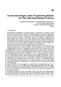
To compute l(j) you need to compare only two things: the old temporary label and the cost of getting to j directly from the most recently labeled nodes. Step V If the target has a permanent label, stop. This label is equal to the minimum cost. Otherwise, return to Step III. The intuition for the algorithm is that a node’s label is an upper bound for the minimum cost of getting from the source to that node. A permanent label is guaranteed to be the true minimum cost of the shortest route (I prove this below). Here is an example. The following figure represents a railroad network. The numbers beside each arc represent the time that it takes to move across the arc. Three locomotives are needed at point 6. There are two locomotives at point 2 and one at point 1. We can use the shortest route algorithm to find the routes that minimize the total time needed to move these locomotives to point 6. �� �� @��2��>> >>1 >> 1 > �/ � � �� 3 �/� � �� ��4�� ��3��
�� �� 3 ��1��> >> >>5 2 >> �� � � �� ��5�� 10
�� � �� �/ �6��
1
4
We must solve two shortest route problems. The shortest route from (1) to (6) and the shortest route from (2) to (6). To use the algorithm, write temporary labels is the table below. Iteration 1 2 3 4 5
1 0∗ 0∗ 0∗ 0∗ 0∗
2 10 10 10 10 10∗∗
3 3∗∗ 3∗ 3∗ 3∗ 3∗
4 ∞ 6 6∗∗ 6∗ 6∗
5 5 5∗∗ 5∗ 5∗ 5∗
6 ∞ ∞ 9 7∗∗ 7∗
The above is a table of labels. Permanent labels are starred and the newest permanent label in each iteration has two stars. All other labels are temporary. In the first iteration, the labels are just c(0, j). In the second iteration, the minimum cost temporary label becomes permanent. The new temporary labels are computed using an extra possible route, namely the direct route from the 9
new permanent label. For example, the label of location (6) decreases from 9 to 7 in Iteration 4 because at that point in the algorithm the possibility of getting from (6) from (4) becomes available. Solution: The shortest distance from (1) to (6) is 7. The route is found by working backwards. Look in the column corresponding to Node (6). Start at the bottom and move until the first time the cost changes. In this example, the cost changes from 7 to 9 between Iterations 3 and 4. Find the node that obtained its permanent label in Iteration 3 (or, generally, when the cost changes). In the example, this is Node (4). This means that the “last stop” before getting to Node (6) is Node (4). Continue to find where the route was immediately before Node (4). Do this by looking in the column corresponding to Node (4) and seeing the last time that the cost changed. In this case that last time the cost changed was between Iteration 1 and Iteration 2. It follows that the route stopped at Node (3) (which was permanently labeled in Iteration 1). Hence the shortest route must be: (1) → (3) → (4) → (6). We also need to find the shortest route from (2) to (6). In this case it is not possible to pass through (1). Iteration 1 2 3
2 0∗ 0∗ 0∗
3 1∗∗ 1∗ 1∗
4 1∗∗ 1∗ 1∗
5 ∞ 3 3∗∗
6 ∞ 2∗∗ 2∗
In the first iteration, we can put a permanent label on both Node (3) and Node (4) since both are minimum cost temporary labels. From the table we see that the shortest distance from (2) to (6) is 2. The shortest route is (2) → (4) → (6). Since we have two locomotives at Node (2) and one at Node (1), the total distance is 7 + 4 = 11. In general, why does the algorithm work? First, it stops in a finite number of iterations. (Since at least one more position receives a permanent label at every iteration of the algorithm and there are a finite number of nodes in the network, after a finite number of steps each node has a permanent label.) Second, and more important, you can show by induction that a permanent label is the cost of a shortest route. At Iteration 1 this is obvious. For all future iterations, it is true. To see this, notice that the newest permanent label (say at Location (N )) gives a cost that is lower than any other route through an existing temporary label. If this label does not represent the cost of a shortest route, then the true shortest route to Location (N ) must pass through a node that does not yet have a permanent label – at a cost greater than that of the minimum temporary label – before reaching Location (N ). Since all cost are nonnegative, this route must cost at least as much as the temporary label at Location (N ). You might ask: What is this problem doing in a discussion of integer programming problems? Given a shortest route problem with costs c(i, j), Node (0) is the source and Node (N ) is the sink. Let x(i, j) = 1 if the path goes from i directly to j and 0 otherwise. The following problem describes the shortest route problem: 10
Find x(i, j) to solve: min
N X N X
c(i.j)x(i, j)
i=0 j=0
subject to: N X
x(i, j) =
i=0
N X
x(j, k)
k=0
for j = 1, . . . N − 1, N X
x(0, k) = 1,
k=1 N −1 X
x(i, N ) = 1,
i=0
and x(i, j) either zero or one. The first constraint says that the number of paths leading to any Node (j) is equal to the number of paths leading out of the node. The second constraint says that at exactly one of the edges in the path must come from the source. The third constraint says that exactly one of the edges in the path must go to the sink. The objective function sums up the cost associated with all of the edges in the path. This formulation requires that all of the costs be non negative.
5
Minimal Spanning Tree Problem
In the minimal spanning tree problem, each edge from Node (i) to Node (j) has a cost (c(i, j)) associated with it and the edge (i, j) represents a way of connecting Node (i) to Node (j). An arc could represent an underground cable that connects a pair of computers. We want to find out a way to connect all of the nodes in a network in a way that minimizes total cost (the sum of the costs of all of the edges used). These definitions explain the name of the problem: A tree is just a collection of edges that is connected and contains no cycles. [This definition has two undefined terms: connected and cycles. The names of these terms are suggestive. Here are definitions, for the pedants: A collection of nodes is connected if you can go from any node to any other node using edges in the collection. A cycle is a collection of edges that starts and ends at the same node.] A spanning tree is a tree that contains all of the nodes in a network. A minimal spanning tree is a spanning tree that has the smallest cost among all spanning trees. There is a simple algorithm for finding minimal spanning trees. Step I Start at any node. Join that node to its closest (least cost) neighbor. Put the connecting node into the minimal spanningc tree. Call the connected nodes C. 11
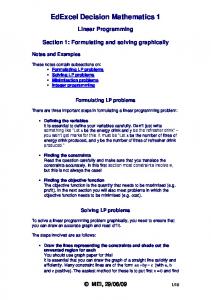
Step II Pick a node j ∗ that is not in C that is closest to C (that is, Node (j ∗ ) solves: min{c(i, j) : i ∈ C, j ∈ / C}). Put Node (j∗) into C and put the cheapest edge that connects C to j∗ into the minimal spanning tree. Step III Repeat this process until a spanning tree is found. If there are N nodes in the network, then the minimal spanning tree with have N − 1 edges. If ties arise in this algorithm, then they may be broken arbitrarily. The algorithm is called greedy because it operates by doing the cheapest thing at each step. This myopic strategy does not work to solve all problems. I will show that it does work (to find the minimum cost spanning tree) for this particular problem. To see how the algorithm works, consider the following example. Suppose that five social science departments on campus each have their own computer and that the campus wishes to have these machines all connected through direct cables. Suppose that the costs of making the connections are given in the network, below. (An omitted edge means that a direct connection is not feasible.) The minimum spanning tree will determine the minimum length of cable needed to complete the connections. �� �� ��1'�� � ' ��� ''' � '
�� �� ��2�� �� � �� � � 2 '' �� 2 ��� �'�' �� �� � '' �� �� 6 �� ��5�� 4 '' 3 �� � 00 '' 0 � �� 0 '' 00 ' ��� ��� 0 ' �� 4�� 2 00 '' 00 ' �� �� 00'' ����� �� �� �� �� 5 ��3�� ��4�� 1
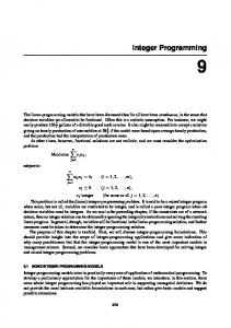
To use the algorithm, start at Node (1). Add Node (2) into the set of connected nodes (because c(1, 2) is smaller than c(1, j) for all other j. This creates the first edge in the minimal spanning tree, which a labeled A below. The minimum cost of connecting Node (3) or Node (4) or Node (5) to Node (1) or Node (2) is two. This minimum is attained when Node (5) is added. Hence we should connect Node (5) next and add either (1, 5) or (2, 5) into the tree. I added (1.5) and called this edge B. The third step connects Node (3) and adds the edge (3, 5) and the final step connects Node (4) and adds the edge (4.5). The diagram below indicates the minimal spanning tree using squiggly connecting segments to indicate the edges in the tree. The letters (in alphabetical order) indicate the order in which new edges were added to the tree. The total cost of the tree is nine.
12
�� �� A �� �� ��1�� /o o/ o/ ��2�� O� O� O� B O� O� O� O� �� �� ��5�� �G �W �G �W �G �W � G �W D G� C �W �G �W �G �W �G �W �� �� �� �� ��4�� ��3�� While the algorithm is intuitively appealing (I hope), it requires an argument to show that it actually identifies a minimal spanning tree. Here is the argument. Denote by Nt the nodes connected in the tth of the algorithm and by Nt0 all of the other nodes. I want to show that each edge added to the tree is part of a minimal spanning tree. Let S be a minimal spanning tree. If the algorithm does not generate S, then there must be a fist step at which it fails. Call this step n. That is, the edges identified in the first n − 1 steps of the algorithm are part of S, but the edges identified in the first n steps are not. Take the edge added at the nth step of the algorithm. This edge connects Nn to Nn0 . Put it into the tree in place of the edge connecting Nn to Nn0 in S. This leads to a new spanning tree S 0 , which must also be minimal (by construction, the algorithm picks the cheapest way to connect Nn to Nn0 ). Consequently, there exists a minimal spanning tree that contains the first n nodes added using the algorithm. As my argument works for any n, it proves that the algorithm generates a minimal spanning tree. There is another algorithm that solves the Minimal Spanning Tree problem. At each stage of the algorithm you pick the cheapest available branch (if there is a tie, break it arbitrarily), provided that adding this branch to your existing tree does not form a cycle. If adding the cheapest branch does create a cycle, then do not add that branch and move on to the next cheapest. Both algorithms presented to solve the Minimal Spanning Tree Problem are “greedy” in the sense that they work by doing the myopically optimal thing without looking for future implications. Problems that can be solved using such an algorithm are combinatorially easy (in the sense that it is computationally feasible to solve large versions of the problem). Not all problems can be solved by a greedy algorithm and the proof that a greedy algorithm works is not always simple. Here are some examples. Consider the problem of making change using standard U.S. coins (penny, nickel, dime, quarter, and if you wish fifty cent piece and dollar). Suppose you wish to use the minimum number of coins. Is there a general procedure that will do this? The answer is yes. One way to describe the procedure is: Continue to use the largest available denomination until the amount that remains is smaller 13
than that denomination. Move to the next lower denomination. Repeat. So, for example, you make change for $4.98 by using 4 dollar coins first. This leaves 98 cents. Next you use a 50 cent piece. That leaves 48 cents. Next a quarter. This leaves 23 cents. Next two dimes, no nickels, and three pennies. If you think that this is obvious, then try to prove that the procedure that I described always works. While you are thinking about the proof, ponder this: In a world where the denominations are perfect squares {1, 4, 9, 16, . . .} the way to make change for 12 cents is to use three 4 cent coins (instead of first using the nine-cent piece and then 4 pennies). Another example is the following scheduling problem: Job j 1 2 3 4 5 6
Deadline dj 1 1 3 2 3 6
Penalty wj 10 9 7 6 4 2
A number of jobs are to be processed by a
single machine. All jobs require the processing time of one hour. Each job j has a deadline dj and a penalty wj that must be paid if the job is not completed by its deadline. For example, consider the problem above, where the deadlines are expressed in hours. A greedy algorithm solves this problem. You can minimize the total penalty costs by choosing the jobs one at a time in order of penalties, largest first, rejecting a job only if its choice would mean that it, or one of the jobs already chosen, cannot be completed on time. The greedy algorithm tells you to do job one (highest penalty); to skip job two (if you do job one you will never finish job two on time); and then to do jobs three and four. Notice that in order to do job four on time you must do it second. This order in fine since after you finish job four you can do job three and still meet job three’s deadline of three. You must skip job five, but you can do job six. To summarize: The algorithm tells you to do jobs 1, 4, 3, and 6 in that order. It should be fairly easy to understand the algorithm. It is somewhat difficult to prove that it actually minimizes the total late penalty. Here is a proof. The proof depends on the following fact: If A1 and A2 are two schedules (an ordering of jobs that can be done on time), and there are more jobs in the second schedule, then it is possible to find another schedule that contains all of the jobs in A1 and one of the jobs in A2 . That is, if it is possible to do, say, ten jobs on time and someone gives you a list of any five jobs that can be done on time, you can add one of the first ten jobs to the second list and still manage to meet all of the deadlines. Here is a proof of the fact. Start with a job done in A2 but not in A1 (such a job exists because there are more jobs in A2 than in A1 ). Suppose that this job is done at time t(1) and call it j(1). If no job is done in A1 at t(1), then 14
schedule j(1) at that time. You are done. If some job is done in A1 at t(1), call it j(2). Either j(2) is not done in A2 or j(2) is done in A2 at time t(2). If j(2) is not done in A2 , then there exits another job j 0 (1) that is done in A2 but not in A1 . So repeat the process above. If j(2) is done in A2 at t(2) ask whether there is a job done in A1 at t(2). If no, then you are done: Add j(1) to A1 at t(1) and reschedule j(2) for t(2). If yes, then repeat as above (call the job done at t(2) j(3)). When finished you will have constructed a chain of jobs, the first member of the chain is done only in A2 , the rest of the chain is done in both schedules. You can enlarge A1 by adding j(1), the first job in the chain and rescheduling the remaining jobs so that no job in the chain is late. To show that the greedy algorithm works, assume that it does not and argue to a contradiction. Suppose that the penalty minimizing schedule, call in A2 , has N jobs in it and the first K < N jobs would be selected by the greedy algorithm but the K + 1 job is not what the algorithm would select. Call the schedule containing the first K + 1 jobs of the greedy algorithm A1 (convince yourself that because K < N , the greedy algorithm can schedule at least one more job). By the fact from the previous paragraph, it is possible to find a schedule that contains these K + 1 jobs, plus an additional N − K − 1 jobs from A2 . The only difference between the augmented schedule A1 and schedule A2 is that the augmented schedule contains the (K + 1)st job added by the greedy algorithm, while A2 contains some job with a larger late penalty. Hence the augmented schedule performs better than A2 . This contradicts the optimality of A2 and completes the proof. The moral of the argument is that it may be easier to use an algorithm than to be able to justify its efficacy.
6
Maximum Network Flow
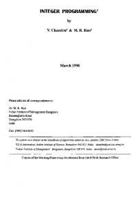
The given information for a maximum flow problem is a network that consists of two distinguished nodes: the starting point or source and the end point, or sink. In this section s denotes the source and n the sink. Edges are directed and have capacities. The maximum flow problem is to specify a nonnegative “load” to be carried on each edge that maximizes the total amount that reaches the sink subject to the constraint that no edge carries a load greater than its capacity. The maximum flow problem is an integer linear programming problem with the property that the solution to the relaxed problem (without integer constraints) will also solve the integer version of the problem. The special structure of the problem allows you to solve it using a simple algorithm. Below is a simple example that I will use to illustrate the algorithm. There are two nodes in addition to the source and the sink. The capacity of the flow from (s) to (1) is 7. The rest of the diagram is easy to understand.
15
�� �� ?��1��?? ?? 9 7 ?? ?? � ����s���� 3 ��?��n���� ?? ?? ? 8 9 ?? �� � � �� ��2�� The algorithm works like this. You begin with no flows. At each iteration you attempt to find an “augmenting path of labeled nodes” from (s) to (n). You use the path to increase flow. You continue this procedure until you cannot find a path of labeled nodes from (s) to (n). In order to describe the algorithm more completely, I must tell you how to label a path. Here are the rules. 1. (s) is always labeled. 2. If Node (i) is labeled, then you can use it to label Node (j) if either: (a) there exists an arc (i) → (j) with excess capacity or (b) there is an arc (j) → (i) with positive flow. Let me illustrate the algorithm using the example. I will put two numbers on each arc. The first represents the current flow. The second represents the arc capacity. A star (*) indicates that the node is labeled. Start with no flow. I have written one augmenting path that goes from (s) → (1) → (2) → (n). I can put three units on this path (because three is the minimum of the used capacities). �� ∗ �� ��> 1 ��B BB 0;9 } (0;7) }} BB BB }} } B } �� ∗ ��} �� ∗ �� (0;3) ��s ��A ��> n �� AA | | AA | A || (0;9) AA || (0;8) � | �� ∗ �� ��2 ��
The next diagram includes the three units shipped by the path found in Step 1. Another augmenting path is (s) → (1) → (n). I can put four units on this path. (If I tried to put more than four units on the path, then I would violate the capacity constraint on (s) → (1).
16
�� ∗ �� ��1 �� }> BBB 0;9 (3;7) }} BB } BB }} B } } �� ∗ �� �� ∗ �� (3;3) ��s ��A ��> n �� AA | | AA | A || (0;9) AA || (3;8) | � �� ∗ �� ��2 �� Now I cannot go from (s) → (1) since that route has no excess capacity. I can go (s) → (2) → (n) and I put five units on this route. �� ∗ �� ��1 �� }> BBB 4;9 (7;7) }} BB } BB }} B } �� ∗ ��} �� ∗ �� (3;3) ��s ��A ��> n �� AA | | AA | A || (0;9) AA || (3;8) � | �� ∗ �� ��2 ��
The next step uses the second way in which you can label a node. [The labeled network below incorporates all of the flows constructed so far.] As in the last step, I cannot label (1) directly because there is no excess capacity on (s) → (1). I can label (2). Furthermore, once (2) has a label, I can label (1) because (1) → (2) has positive flow. (n) can receive a label because (1) → (n) has excess capacity and (1) is labeled. The most I can put on the (s) → (2) → (1) → (n) route is three since three is the flow from (1) → (2). �� �� ��> 1∗ ��B BB 4;9 } (7;7) }} BB } BB } } B } �� ∗ ��} �� ∗ �� (3;3) ��> n �� ��s ��A AA | AA || | A | (5;9) AA || (8;8) �� �∗ ��| ��2 ��
When we add the three units we obtain the next diagram. This is the final step. Notice that we can label (s) and (2) but no other nodes. Hence it is not possible to find an augmenting path from (s) to (n). The diagram indicates the optimal flow. The total that can reach the sink is 15 (add up the amounts shipped on all of the nodes that reach (n) directly. In this case (1) → (n) and (2) → (n).
17
�� �� >��1��@@ } @@ 7;9 (7;7) }} @@ }} } @@ } � �� ∗ ��} (0;3) ��?��n���� ��s ��A ~ AA ~~ AA ~~ AA ~ (8;9) A � ~~ (8;8) �� ∗ �� ��2 �� Now that you have followed this far, let me confess that you could do this problem in two steps. In the first step, increase the flow to seven by using the path (s) → (1) → (n). In the second step, increase the flow to fifteen by using the path (s) → (2) → (n). I did the problem the long way to illustrate the possibility of labeling through “backwards” arcs as in Step 4 and to demonstrate that the procedure will work to produce a solution no matter what order you generate augmenting paths. When the given capacities are integers, the algorithm is guaranteed to finish in a finite number of steps and provide an answer that is also an integer. There is also a way to prove that your answer is correct. Define a cut to be a partition of the nodes into two sets, once set containing (s) and the other set containing (n). The cut capacity is the total capacity frow the part of the cut containing the source to the part of the cut containing the sink. Convince yourself that the capacity of any cut is greater than or equal to any feasible flow. Hence finding any cut can give you an upper bound on the maximum flow. For example, consider the cut {(s)} ∪ {(1), (2), (n)}. It has capacity 16, so the maximum flow cannot exceed 16. Since the capacity of any cut is greater than or equal to the maximum flow, if you can ever find a cut that has capacity equal to a feasible flow, then you know that you have solve the problem. This is exactly what happens at the end of the algorithm. Whenever you reach a point where you can no longer find a flow augmenting path, you are able to generate a cut by taking as one set the set of labeled nodes and the other set the rest. For example, for the final diagram of the example, the cut is {(s), (2)} ∪ {(1), (n)} has capacity fifteen. You should be able to convince yourself that a cut created in this fashion has capacity equal to the maximum flow (otherwise you would have been able to label another node). The general fact that the minimum capacity cut is equal to the maximum flow is a consequence of the duality theorem of linear programming. One application of the maximum flow problem is a kind of assignment problem. Suppose that there are m jobs and n people. Each person can be assigned to do only one job and is only able to do a particular subset of the jobs. The question is: What is the maximum number of possible jobs that can be done. The way to solve this problem using network flows is to set up a network in which there is an arc with capacity one connecting the source to each of the n nodes (one for each person), an arc with capacity one connecting each person to each job that the person can do, and an arc with capacity one connecting 18
each job to the sink. For example, the network below represents the situation in which there are four people and five jobs. The first person can do only job A. The second person can do either job A or job B, the third person can do either job C or job D, and the fourth person can do either job D or job E. Plainly, you can get four jobs done in this situation. The solution is not so obvious when there are more people and more jobs. It is not difficult to modify the algorithm to accommodate the situation in which some people can be assigned to do more than one job. (It is slightly harder to deal with the situation in which the number of jobs that a person can do depends on which jobs that person is assigned to do.) �� �� �? �A �� �G /// 1 � // � �� / �� �� 1 �� �� �� //1 @���1�� �� �?�B ��?? // ?? 1/ � 1 1 ��� ?? // �� � ??/ � � � � �� �� 1 �/ �� � �� ����s����� 1 �/ � �� �?�n ��2�� ��C �� G �� ..== ? � ..===1 1 �� 1 .. === � .. 1 �� � �� 1 �� ��1 ��� /��D�� � .. ��3�� ? �� .. 1 � .. �� ��� �� 1 �/ � ��� ��4�� ��E ��
Another application of the approach is to solve a type of transshipment problem. You are given a number of warehouses, each with a fixed supply of something. Your are given a number of markets, each with a fixed demand for that thing. You are given the capacity of the various shipping routes (from warehouse i to market j). Your problem is to determine whether it is possible to meet the given demand. For example, the information could be:
Warehouse 1 2 3 Demands
1 30 0 20 20
Markets 2 10 0 10 20
Supplies 3 0 10 40 60
4 40 50 5 20
20 20 100
The information in the table can be interpreted as follows. There are three warehouses. Reading down the last column we see that the supply available at each one (so warehouse one has supply 20). There are four markets. Reading across the last row we see the demand available at each one (so the demand in Market 3 is 60). The numbers in the table describe what can be shipped directly 19
from one warehouse to a market (so you can ship as many as forty units from the third warehouse to the third market). As is the case in the assignment problem, we construct a network from this information. From the sin there is an arc to a node for each warehouse. The capacity of the arc is the supply at he warehouse. From each warehouse node there is an arc to a node fro each market. The capacity of the arc is the maximum feasible flow to that market. From each market node there is an arc to the sink with capacity equal to the demand in that market. For the example, therefore, the relevant network is: �� �� �� �� 30 ��G 1��- MMM �/ �H1��/ �� -- MMM 10 � / MMM �� // -// ��� M � MM� M -� � � � �� & 20 � -� ��2�� // 20 ��� -��� E >>> /// >> / � -- �� > 20 >>// ��� -- �� � �� ����s���� 20 �/ � �� ����� n �� ��2��