Oct 18, 2011 - acting 2D Dirac electron liquid develops a magnetic re- ... also in the electronic structure of graphene. ...... 36 G. Gui, J. Li, and J. Zhong, Phys.
Linear response correlation functions in strained graphene F. M. D. Pellegrino,1, 2 G. G. N. Angilella,1, 2, 3, 4 and R. Pucci1, 2
arXiv:1110.4036v1 [cond-mat.mes-hall] 18 Oct 2011
1
Dipartimento di Fisica e Astronomia, Universit` a di Catania, Via S. Sofia, 64, I-95123 Catania, Italy 2 CNISM, UdR Catania, I-95123 Catania, Italy 3 Scuola Superiore di Catania, Universit` a di Catania, Via Valdisavoia, 9, I-95123 Catania, Italy 4 INFN, Sez. Catania, I-95123 Catania, Italy (Dated: October 19, 2011)
After deriving a general correspondence between linear response correlation functions in graphene with and without applied uniaxial strain, we study the dependence on the strain modulus and direction of selected electronic properties, such as the plasmon dispersion relation, the optical conductivity, as well as the magnetic and electric susceptibilities. Specifically, we find that the dispersion of the recently predicted transverse plasmon mode exhibits an anisotropic deviation from linearity, thus facilitating its experimental detection in strained graphene samples. PACS numbers: 73.20.Mf, 62.20.-x, 81.05.ue
I.
INTRODUCTION
Graphene is a truly two-dimensional (2D) electronic system, based on an atomically thin carbon honeycomb lattice1 . Low-energy quasiparticles can be described as massless Dirac fermions, with a cone dispersion relation in reciprocal space around the so-called Dirac points K, K′ , and a linearly vanishing density of states (DOS) at the Fermi level2,3 . Such a linear spectrum and reduced dimensionality yield remarkable behaviors already in the non-interacting limit of several electronic properties of graphene. These include, inter alia, the reflectivity4 , the optical conductivity5–9 , the plasmon dispersion relation10–13 , as well as a newly predicted transverse electromagnetic mode14 , which is characteristic of a 2D system with a double band structure, such as graphene. Moreover, the relevance of lossless plasmons in graphene in the infrared frequency range has been emphasized, with possible applications in nanophotonics15,16 . These properties can be extracted from the study of the appropriate correlation functions within linear response theory17–19 . Within the Dirac approximation, rotational invariance implies thet the current-current correlation function may be decomposed in a longitudinal and a transverse contribution, the former being related to the density-density correlation function via the continuity equation18,20 . Moreover, in the case of massless Dirac fermions, it has been observed that the current-current response is simply proportional to its pseudospin-pseudospin counterpart20 . On the other hand, the magnetic susceptibility is related to the transverse contribution18,21,22 . Specifically, the noninteracting Dirac model yields an orbital magnetic susceptibility χm (q → 0) ∝ δ(µ), in the long wavelength limit20 . This is consistent with earlier results for graphite23 , obtained using Wallace’s two-dimensional band structure for a graphene layer24. Such a finding would predict no response to a uniform, static magnetic field, away from half-filling. This is of course par-
tially compensated by a smearing of the δ-function at finite temperatures, already in the noninteracting limit. Still at zero temperature and in the noninteracting limit, one recovers a nonzero magnetic response also away from half-filling, when the honeycomb lattice structure is considered25 . The effect of the interactions has been considered in Ref. 26, where it is shown that an interacting 2D Dirac electron liquid develops a magnetic response also at finite doping. Concerning the response to an external electromagnetic field, graphene is also unique among other conventional 2D electron systems, in that it has been predicted that it can sustain a transverse plasmon mode14 , as a consequence of its double band structure. More recently, such a transverse mode has been predicted also for bilayer graphene27 . Here, we will consider the effect of strain on the various electronic properties that may be described by linear response correlation functions. Indeed, a deformation of the lattice through the application of uniaxial strain or hydrostatic pressure is expected to produce modifications also in the electronic structure of graphene. Recently, it has been proposed that nanodevices based on graphene could be engineered on the basis of the expected straininduced modifications of the deformed graphene sheet (origami electronics)28 . This is made possible by the exceptional mechanical properties of graphene, as is the case for other carbon compounds. For instance, despite its reduced dimensionality, graphene is characterized by a sizeable tensile strength and stiffness29 , with graphene sheets being capable to sustain elastic deformations as large as ≈ 20%30–34 . Larger strains would then induce a semimetal-to-semiconductor transition, with the opening of an energy gap35–38 , and it has been demonstrated that such an effect critically depends on the direction of applied strain5,39 . The paper is organized as follows. In Sec. II we present our formalism for treating graphene under uniaxial strain, and derive our central result for a generic linear response function for a deformed graphene sheet.
2 This, in particular, applies to the density-density and current-current correlation functions. In Sec. III we then study the electron polarization, with emphasis on the strain dependence of the plasmon dispersion relation and the conductivity. Specifically, we find a strain-induced anisotropic enhancement of the deviations from linearity of the transverse plasmon14 , which should facilitate its experimental detection. In Sec. IV we derive the strain dependence of the magnetic and electric susceptibilities. Finally, we summarize our results in Sec. V.
II.
ck = 1 − 2κε, c⊥ = 1 + 2κνε,
H (0) = ~vF σ · q,
(1)
where vF is the Fermi velocity, σ = (σx , σy ), with σx , σy Pauli matrices, and q is the wavevector displacement from the Dirac point one is referring to, i.e. k = K + q. Here and below, a superscript zero denotes absence of strain. The effect of strain is then that of modifying (0) the lattice vectors as δ ℓ = (I + ε) · δ ℓ (ℓ = 1, 2, 3), √ √ (0) (0) (0) where δ 1 = a( 3, 1)/2, δ 2 = a(− 3, 1)/2, δ 3 = a(0, −1) are the relaxed (unstrained) vectors connecting two nearest-neighbor (NN) carbon sites, with a = 1.42 ˚ A, the equilibrium C–C distance in a graphene sheet2 , and ε is the strain tensor35 1 ε[(1 − ν)I + (1 + ν)A(θ)], 2
(2)
where A(θ) = σz e2iθσy = cos(2θ)σz + sin(2θ)σx .
(3)
In Eq. (2), θ denotes the angle along which the strain is applied, with respect to the x axis in the lattice coordinate system, ε is the strain modulus, and ν is Poisson’s ratio. While in the hydrostatic limit ν = −1 and ε = εI, in the case of graphene one has ν = 0.14, as determined from ab initio calculations40 , to be compared with the known experimental value ν = 0.165 for graphite41 . The special values θ = 0 and θ = π/6 refer to strain along the zig zag and armchair directions, respectively. The overall effect of a moderately low applied uniaxial strain on the low-energy Hamiltonian is that of shifting the location of the Dirac point in momentum space as K → kD , and changing the shape of the Dirac cone, into a deformed one, with elliptical section5 . Such a picture applies for strain moduli below the value at which a gap opens in the energy spectrum, which takes place at ε ≃ 20%30–34 . In particular, setting k = kD + q, with q measuring now the vector displacement from the shifted Dirac point, the Fermi velocity, defined as the slope of the Dirac cone in the direction of q, will now have anisotropic
(4a) (4b)
where κ = (a/2t)|∂t/∂a| − 12 ≈ 1.1 is related to the logarithmic derivative of the nearest-neighbor hopping t at ε = 0. Thus, the low-energy Hamiltonian around kD maintains a linear form even in the presence of strain, and can still be written as
MODEL
The low-energy Hamiltonian for noninteracting quasiparticles around a Dirac point, say K, has the well-known linear form2
ε=
components ck vF , c⊥ vF along the direction of applied strain and the direction orthogonal to it, respectively, with
H = ~vF σ · q′ ,
(5)
q′ = R(θ)S(ε)R(−θ)q,
(6)
where now
with R(θ) the rotation matrix in the direction of applied strain, and S(ε) = diag (ck , c⊥ ) the matrix describing the deformation of the Dirac cone. Explicitly, for the compound transformation matrix R(θ)S(ε)R(−θ) mapping q onto q′ one finds R(θ)S(ε)R(−θ) = I − 2κε.
(7)
A central result of the present work is that a similar correspondence holds between a generic linear response function χ(q, ω) under applied strain, with respect to its unstrained limit, χ(0) (q, ω). This follows from the fact that any linear response function χ(q, ω) of a noninteracting electron system can be expressed as an integral over the first Brillouin zone (1BZ) of a suitable matrix operator over pseudospins, which is itself a function of q. Such an operator then admits a unique expression in terms of the Pauli matrices σx , σy , σz , and the identity matrix I ≡ σ0 . The simplest cases are then given by the density operator and the density current operator, which in reciprocal space read20 X † ρ(0) (q) = Ψk−q IΨk , (8a) k
(0) Ji (q)
= −evF
X
Ψ†k−q σi Ψk ,
i = x, y,
(8b)
k
respectively, where Ψ†q = (ψqA , ψqB ), and ψqα destroys a quasiparticle with momentum q and pseudospin α = A, B, and summations run over the 1BZ. While the density operator does not change under applied strain, for the generic component of the density current operator one has (0)
Ji = [I − 2κε]ij Jj .
(9)
Here and below a summation will be understood over repeated indices (j = x, y). Defining now eigenvalues and eigenvectors in pseudospin space of the Hamiltonian with and without applied strain, Eqs. (1) and (5), as H (0) |q′ , λi(0) =
3 (0)
Eλq′ |q′ , λi(0) and H|q, λi = Eλq |q, λi, respectively, with λ a pseudospin index, it follows that both Eλq and |q, λi (0) under applied strain are mapped onto Eλq′ and |q′ , λi(0) , ′ respectively, where q is given in terms of q by Eq. (6). Performing such a linear change of variables in the integral defining the correlation function of interest, in the cases of the density-density and current-current correlation function, it follows therefore that Πρρ (q, ω) = [det S(ε)]
−1
Πij (q, ω) = [det S(ε)]
−1
′ Π(0) ρρ (q , ω),
(10a)
(0)
×[I − 2κε]ih Πhk (q′ , ω)[I − 2κε]kj(10b) , where det S(ε) = (1 − 2κε)(1 + 2κνε). From Eq. (10a), in the case of the density-density correlation function, it follows in particular that the effect of applied strain is that of transforming the momentum variable q into an ‘effective’ one q′ , plus the introduction of an overall scale −1 factor [det S(ε)] , which is isotropic with respect with the strain direction. Such a scale factor is directly related to the slope of the electronic density of states at the Fermi level. As is well known, this goes linearly with the chemical potential µ, and it has been shown that its steepness increases with increasing strain, for moderately low strain modulus5 . In the case of the current-current correlation function, such an overall effect is then superimposed to an anisotropic deformation, depending on the angle of applied strain, θ, as shown by Eq. (10b). Linearizing Eq. (10) with respect to ε, one finds Πρρ (q, ω) = [1 + 2κ(1 − ν)ε] Π(0) ρρ (q, ω) −2κ
(0) ∂Πρρ (q, ω)
∂qh
εhk qk ,
(11a)
(0)
Πij (q, ω) = [1 + 2κ(1 − ν)ε] Πij (q, ω) (0)
∂Πij (q, ω) εhk qk −2κ ∂qh −2κ{ε, Π(0) (q, ω)}ij ,
(11b)
where the curly brackets in the last term denote a matrix anticommutator.
III. A.
POLARIZATION
Charge response: Plasmons and conductivity
We now specifically turn to consider the densitydensity correlation function within linear response theory, i.e. the electron polarization Πρρ (q, ω). Plasmon modes are then recovered as poles of the polarization, and the effect of strain on their dispersion relation has been studied in Refs. 10,11. In particular, by including local field effects, as a consequence of the two-band character of the band structure of graphene, we found two
main plasmon branches, the lower branch being characterized by the standard square-root dependence on q, at long wavelengths, as expected for a two-dimensional system10 . In given limits, the asymptotic form of the noninteract(0) ing polarization in the absence of strain, say Πρρ (q, ω) is known explicitly. For instance, in the long wavelength limit (q → 0), one finds17 � 2µ − ~ω gs gv q 2 2µ 1 (0) Πρρ (q → 0, ω) = + log 8π~ω ~ω 2 2µ + ~ω i π (12) −i Θ(~ω − 2µ) , 2 where gs = gv = 2 take into account for spin and val(0) ley degeneracies, respectively. In other words, Πρρ (q → 2 0, ω) = Z(ω)q , at a given ω, with the complex factor Z(ω) implicitly defined by Eq. (12). In the case of applied strain, but still in the noninteracting limit, this is then readily modified through the linearized Eq. (11), yielding
Πρρ (q → 0, ω) = [1 − 2κ(1 + ν)ε cos(2θ − 2ϕ)] Z(ω)q 2 , (13) where q ≡ q(cos ϕ, sin ϕ). Within the random phase approximation (RPA), the interacting polarization reads ¯ ρρ (q, ω) = Πρρ (q, ω)/(1 − V (q)Πρρ (q, ω)), where Π V (q) = e2 /(2ǫr ǫ0 q) is the (bare) Coulombic electronelectron interaction, and ǫr is the dielectric constant of the medium. Solving for the plasmon dispersion relation, ¯ −1 (q, ω) = 0, at low energies one finds Re Π ρρ r
√ e2 µ [1 − κ(1 + ν)ε cos(2θ − 2ϕ)] q 2πǫ √ (14) ≡ ~˜ ω1 (ϕ) qa.
~ωpl =
√ One thus finds that the prefactor ω ˜ 1 (ϕ) in the qdependence is maximum [resp., minimum] for ϕ−θ = π/2 [ϕ−θ = 0], i.e. wavevector orthogonal [parallel] to the direction of applied strain. Correspondingly, one also finds for the imaginary part of the retarded polarizability along the low-energy plasmon branch
¯ ρρ (q, ω + i0+ ) = Im Π r 1 2πǫ − µ [1 − κ(1 + ν)ε cos(2θ − 2ϕ)] 2 e2 ×(qa)3/2 δ(~ω − ~ωpl (q)). (15) Therefore, one recovers a dependence of the plasmon spectral weight on the angle of applied strain, similar to that shown by ω ˜ 1 (ϕ) in Eq. (14). Another quantity of interest which is related to the density-density correlation function is the optical conductivity, which can be obtained as σϕϕ (ω) =
ie2 ω2 lim 2 Πρρ (q, ω). ω q→0 q
(16)
4 Making use of Eq. (11) and (12) one therefore finds the optical conductivity in the presence of applied strain as
where σ0 = πe2 /2h is proportional to the quantum of conductivity. In the hydrostatic limit, ν = −1, σϕϕ does not depend on strain, as may be expected, as the unstrained relation does not contain the Fermi velocity. The above expression for the conductivity, Eq. (17), can be exploited to study the strain dependence of the transverse electromagnetic mode, that has been recently predicted theoretically in graphene14 , and in a graphene bilayer27 . In a 2D electron gas, the spectrum of electromagnetic modes obeys the equations42 σ ζ(q, ω) = 0, 2ǫ0 ω ω σ = 0, 1−i 2ǫ0 ζ(q, ω)c2 1+i
(18a) (18b)
for the longitudinal and transverse plasmons, respectively, where ζ 2 (q, ω) = q 2 − (ω/c)2 , where c is the velocity of light in vacuum. While conventional 2D electron systems cannot sustain a transverse electromagnetic mode, it has been predicted14 that graphene can develop a transverse plasmon mode, as a consequence of a negative imaginary part in the interband contribution to its optical conductivity, Eq. (17). Its logarithmic divergence as ~ω/µ → 2 is in turn related to the discontinuous behavior of the interband absorption of radiation at frequencies ~ω > 2µ. Such a feature is a generic consequence of causality, and is related through a KramersKr¨onig transformation to the step-like behaviour of the real part of the optical conductivity. This is in turn due to the existence of a Fermi surface, which is however expected to be smeared at finite temperature, thus implying the reduction of the logarithmic singularity into a pronounced (but finite) peak. Indeed, making use of Eq. (17) in Eq. (18a), one consistently recovers Eq. (14) for the longitudinal plasmons. On the other hand, substituting Eq. (17) in Eq. (18b), one obtains the strain-dependence of the dispersion relation of the transverse plasmon implicitly as ~c ζ(q, ω) = (1 − 2κ(1 + ν)ε cos(2θ − 2ϕ)) αµ � � 2µ + ~ω ~ω −2 , log × 2µ 2µ − ~ω
(19)
where α = e2 /(4πǫ0 ~c) is the fine structure constant. Because of the small factor α in the left-hand side of Eq. (19), the dispersion relation of such a transverse mode is close to the linear dispersion relation of the electromagnetic radiation itself, ω − cq . 0. However, one may expect that applied strain enhances deviations from linearity (i.e., from the photon’s dispersion relation), as a
-0.2 103 −h ( ω - c q ) / µ
σϕϕ (ω) = σ0 [1 − 2κ(1 + ν)ε cos(2θ − 2ϕ)] � � 2µ − ~ω i 4 µ , (17) + log × Θ(~ω − 2µ) + i π ~ω π 2µ + ~ω
0
-0.4 -0.6 -0.8 -1 -1.2 -1.4 1.65
1.7
1.75
1.8
1.85
1.9
1.95
2
2.05
−
hcq/µ
FIG. 1: Showing deviations from linearity of the frequency of the transverse plasmon, Eq. (19), for q in the allowed range, for strain modulus ε = 0.1, and strain direction ranging from ϕ − θ = 0 (top) to ϕ − θ = π/2 (bottom).
consequence of a strain-induced modification of the band dispersion. Fig. 1 shows indeed deviations from linearity, ω − cq of the transverse plasmon, for q in the allowed range, for strain modulus ε = 0.1, and strain direction 0 ≤ ϕ − θ ≤ π/2. One finds indeed that, in the case of applied strain, deviations of the transverse plasmon dispersion relation from that of the electromagnetic radiation become significant over a sufficiently wide window in ~cq/µ . 2, especially when ϕ − θ = π/2. Therefore, applied strain should help the experimental detection of this elusive collective mode. Indeed, the fact that the plasmon dispersion relation is close to the corresponding electromagnetic dispersion implies that such a transverse plasmon mode would have a marked photonic character, and a small plasmon linewidth would therefore hinder its observation43 . On the other hand, at finite temperature, the real part of the optical conductivity is nonzero also for ~ω . 2µ, so that the transverse plasmon mode does acquire a finite, albeit small, linewidth14 . In particular, this applies to plasmon energies such that 0 < 2µ − ~ω < kB T . This is exactly where the plasmon dispersion relation deviates most from its photonic counterpart, the deviation being enhanced, and shifted away from the limiting case ~ω = 2µ, in the case of applied strain, for q perpendicular to the strain direction. One therefore expects wavevectors of the order of ~cq . 2µ, or equivalently q/kF . 2vF /c ≪ 1, so that it is justified to employ Eq. (19)14,17 .
B.
Current response
In the case of an applied vector field (e.g., an electric field Ei ), one may in general decompose the linear response function in a longitudinal and a transverse component as � � qi qj qi qj χij (q, ω) = 2 χk (q, ω) + δij − 2 χ⊥ (q, ω), (20) q q
5 where q = |q|, for a homogeneous system44 . In particular, in the case of the current-current correlation function, the latter being proportional to the pseudospinpseudospin counterpart, this can be further simplified as (0)
(0)
(0)
Πij (q, ω) = Π+ (q, ω)δij + Π− (q, ω)Aij (ϕ),
Therefore, as a consequence of Eq. (10), it follows that even though an unstrained system is characterized only by transverse response in the static limit45 , it may develop a nonzero parallel response as a result of a straininduced deformation. Making use of Eq. (11b), one finds
(21)
where (0)
Π± (q, ω) =
1 (0) (0) [Π (q, ω) ± Π⊥ (q, ω)]. 2 k
(22)
h i (0) (0) (0) (0) Πij (q, ω) = Πij (q, ω) − 2εκ(1 + ν) Π− (q, ω) cos(2θ − 2ϕ)δij + Π+ (q, ω)Aij (θ) + Π− (q, ω)Aij (ϕ + π/4) sin(2θ − 2ϕ) # " (0) (0) ∂Π− (q, ω) ∂Π+ (q, ω) δij + q Aij (ϕ) . (23) −κ[(1 − ν) + (1 + ν) cos(2θ − 2ϕ)]ε q ∂q ∂q In the static limit (ω = 0), Eq. (23) can be further simplified, by considering the analytic result of Ref. 20, with (0) Πk (q, 0) = 0, and 2
(0)
Π⊥ (q, 0) =
gs gv e vF 2 1 − Θ (~vF q − 2µ) arcsin 16~q π
�
In particular, one recovers a vanishing response, Πqq (q, 0) = 0, with Πqq denoting the current-current correlation function for both vector potential and response field aligned with q, when q is aligned with the applied field also in the presence of strain, as expected in the static limit. IV.
ELECTRIC AND MAGNETIC SUSCEPTIBILITIES
A magnetic field applied in the direction perpendicular to the graphene plane can be described as Bext (q) = Bext (q)ˆz = iq × A, where A = i(qy , −qx )Bext /q 2 , in reciprocal space. The linear response to such a magnetic field is then given by a current Ji , which in turn produces a magnetization term δB ≡ χm Bext . In the case of a static, uniform magnetic field, oriented in the direction orthogonal to the graphene sheet, one is interested in the magnetic susceptibility defined as Z dϕ χM = lim χm (q, 0). (25) q→0 2π
Making use of Eq. (24), one obtains � � �� µ0 ∂ Π⊥(0) (q, 0). 1 − κ(1 − ν)εq χM = lim − 2 q→0 q ∂q (26) In the strained case, this reads χM = −µ0 [1 − 2κ(1 − ν)ε]
gs gv e2 vF2 δ(µ). 6π
(27)
2µ ~vF q
�
−
2µ ~vF q
s
1−
�
2µ ~vF q
�2
− Θ (2µ − ~vF q) .
(24)
One therefore obtains a qualitatively similar result to the case of undeformed graphene, treated within the Dirac approximation and neglecting the electron-electron interaction20,23 . On the other hand, applied strain causes a reduction of the magnetic response, Eq. (26). Although Eq. (27) would imply no response to a static, uniform magnetic field away from half-filling, one expects that finite-temperature effects would broaden the δ-function, already in the noninteracting limit. A qualitatively similar smearing of the peak in the dependence on the chemical potential may also be induced by disorder46 . Still at zero temperature and in the noninteracting limit, one recovers a nonzero magnetic response also away from half-filling, when the honeycomb lattice structure is considered25 . The effect of the interactions has been considered in Ref. 26, where it is shown that an interacting 2D Dirac electron liquid develops a magnetic response also at finite doping.
An analogous procedure may be followed to derive the electric susceptibility χe , entering the relationship δE = χe Eext between the electric polarization and an external electric field. One is then interested in the static (ω = 0) limit of the density-density polarization. In the presence of applied strain, at arbitrary µ = ~vF kF , using Eq. (11), one explicitly finds
6
� � � � gs gv q + 2µ gs gv µ Θ(~v q − 2µ) G + Πρρ (q, ω = 0) = [1 + 2κ(1 − ν)ε] − F 2π~2 vF2 8π~vF < ~vF q � � 2µ gs gv q − G −κ[(1 − ν) + (1 + ν) cos(2θ − 2ϕ)]ε Θ(~vF q − 2µ), 8π~vF < ~vF q
where17,18 p 2 G± < (x) = ±x 1 − x − arccos x,
|x| < 1.
(29)
In particular, at zero doping (µ = 0, G± < (0) = −π/2), one finds in general that χe (q, 0) = V (q)Πρρ (q, 0).
(30)
It should be emphasized that, while Eq. (30) describes the response of the system to a static electric field lying in the same graphene layer. More explicitly, in the undoped case, Eq. (30) reads gs gv e2 q→0 32ǫ0 ǫr ~vF × [1 + κ(1 − ν)ε − κ(1 + ν)ε cos(2θ − 2ϕ)] ,(31)
χe = lim χe (q, 0) = −
tion functions of graphene. After deriving a general correspondence between strained and unstrained correlation functions, we have derived the strain dependence of the plasmon dispersion relation and of the optical conductivity. Specifically, we find that the prefactor in √ the q-dependence of the plasmon frequency develops an anisotropic character, with maxima occurring when the wavevector is orthogonal to the direction of applied strain. Moreover, we derive a strain-induced anisotropic enhancement of the deviations from linearity of the recently predicted transverse plasmon14 , which should facilitate its experimental detection in suitably strained graphene samples. Finally, we have compared and contrasted the strain dependences of the magnetic and electric susceptibilities, showing that strain enhances the response of strained graphene to an applied electric field, while suppressing the response to an magnetic field. Acknowledgments
where ϕ is the direction of the electric field on the graphene plane, thus showing that uniaxial strain introduces a modulation in the angle of applied strain. Moreover, comparison with Eq. (26) in the hydrostatic limit (ν = −1) shows that strain enhances the electric response, while suppressing the magnetic one. V.
CONCLUSIONS
We have studied the dependence on applied uniaxial strain of several linear-response electronic correla-
1
2
3
4
5
6
7
K. S. Novoselov, D. Jiang, F. Schedin, T. J. Booth, V. V. Khotkevich, S. V. Morozov, and A. K. Geim, Proc. Nat. Acad. Sci. 102, 10451 (2005). A. H. Castro Neto, F. Guinea, N. M. R. Peres, K. S. Novoselov, and A. K. Geim, Rev. Mod. Phys. 81, 000109 (2009). D. S. L. Abergel, V. Apalkov, J. Berashevich, K. Ziegler, and T. Chakraborty, Adv. Phys. 59, 261 (2010). R. R. Nair, P. Blake, A. N. Grigorenko, K. S. Novoselov, T. J. Booth, T. Stauber, N. M. R. Peres, and A. K. Geim, Science 320, 1308 (2008). F. M. D. Pellegrino, G. G. N. Angilella, and R. Pucci, Phys. Rev. B 81, 035411 (2010). T. Stauber, N. M. R. Peres, and A. K. Geim, Phys. Rev. B 78, 085432 (2008). A. B. Kuzmenko, E. van Heumen, F. Carbone, and D. van der Marel, Phys. Rev. Lett. 100, 117401 (2008).
(28)
FMDP acknowledges Dr D. M. Basko for inspiring discussions, and for carefully reading the manuscript. FMDP also thanks the Laboratoire de Physique et Mod´elisation des Mileux Condens´es, CNRS, Grenoble (France) for much hospitality and for the stimulating environment.
8
9
10
11
12
13
14
15
F. Wang, Y. Zhang, C. Tian, C. Girit, A. Zettl, M. Crommie, and Y. R. Shen, Science 320, 206 (2008). K. F. Mak, M. Y. Sfeir, Y. Wu, C. H. Lui, J. A. Misewich, and T. F. Heinz, Phys. Rev. Lett. 101, 196405 (2008). F. M. D. Pellegrino, G. G. N. Angilella, and R. Pucci, Phys. Rev. B 82, 115434 (2010). F. M. D. Pellegrino, G. G. N. Angilella, and R. Pucci, High Press. Res. 31, 98 (2011). E. H. Hwang and S. Das Sarma, Phys. Rev. B 75, 205418 (2007). S. H. Abedinpour, G. Vignale, A. Principi, M. Polini, W.-K. Tse, and A. H. MacDonald, Phys. Rev. B 84, 045429 (2011), URL http://link.aps.org/doi/10.1103/PhysRevB.84.045429. S. A. Mikhailov and K. Ziegler, Phys. Rev. Lett. 99, 016803 (2007). M. Jablan, H. Buljan, and M. Soljaˇci´c, Phys. Rev. B 80,
7
16
17
18
19
20
21
22
23 24 25
26
27
28
29
30
31 32
Phys. Rev. Lett. 102, 235502 (2009). 245435 (2009). 33 S.-M. Choi, S.-H. Jhi, and Y.-W. Son, Phys. Rev. B 81, Z. Q. Li, E. A. Henriksen, Z. Jiang, Z. Hao, M. C. Martin, 081407(R) (2010). P. Kim, H. L. Stormer, and D. N. Basov, Nature Phys. 4, 34 J.-W. Jiang, J.-S. Wang, and B. Li, Phys. Rev. B 81, 532 (2008). 073405 (2010). B. Wunsch, T. Stauber, F. Sols, and F. Guinea, 35 V. M. Pereira, A. H. Castro Neto, and N. M. R. Peres, New Journal of Physics 8, 318 (2006), URL Phys. Rev. B 80, 045401 (2009). http://stacks.iop.org/1367-2630/8/i=12/a=318. 36 G. Gui, J. Li, and J. Zhong, Phys. Rev. B 78, 075435 T. Stauber and G. G´ omez-Santos, Phys. Rev. B 82, 155412 (2008). (2010). 37 R. M. Ribeiro, V. M. Pereira, N. M. R. Peres, P. R. BridSee also Appendix E in Ref. 47, for a systematic classificadon, and A. H. C. Neto, New J. Phys. 11, 115002 (2009). tion. 38 G. Cocco, E. Cadelano, and L. Colombo, Phys. Rev. B 81, A. Principi, M. Polini, and G. Vignale, Phys. Rev. B 80, 241412 (2010). 075418 (2009). 39 F. M. D. Pellegrino, G. G. N. Angilella, and R. Pucci, High M. Koshino, Y. Arimura, and T. Ando, Phys. Rev. Lett. Press. Res. 29, 569 (2009). 102, 177203 (2009). 40 M. Farjam and H. Rafii-Tabar, Phys. Rev. B 80, 167401 T. Ando, Journal of the Physical Soci(2009). ety of Japan 75, 074716 (2006), URL 41 O. L. Blakslee, D. G. Proctor, E. J. Seldin, G. B. Spence, http://jpsj.ipap.jp/link?JPSJ/75/074716/. and T. Weng, J. Appl. Phys. 41, 3373 (1970). J. W. McClure, Phys. Rev. 104, 666 (1956). 42 V. I. Fal’ko and D. E. Khmel’nitski˘ı, Sov. Phys. JETP 68, P. R. Wallace, Phys. Rev. 71, 622 (1947). 1150 (1989), [Zh. Eksp. Teor. Fiz. 95, 1988 (1989)]. G. G´ omez-Santos and T. Stauber, Phys. Rev. Lett. 106, 43 M. Jablan, M. Soljaˇci´c, and H. Buljan, Phys. Rev. B 83, 045504 (2011). 161409 (2011). A. Principi, M. Polini, G. Vignale, and M. I. Katsnelson, 44 G. Giuliani and G. Vignale, Quantum Theory of the Phys. Rev. Lett. 104, 225503 (2010). Electron Liquid (Cambridge University Press, Cambridge, M. Jablan, H. Buljan, and M. Soljaˇci´c, 2005). Opt. Express 19, 11236 (2011), URL 45 The static (ω → 0) longitudinal response describes the rehttp://www.opticsexpress.org/abstract.cfm?URI=oe-19-12-11236. sponse of the system to a static longitudinal vector potenV. M. Pereira and A. H. Castro Neto, Phys. Rev. Lett. tial, which can always be removed via a gauge transforma103, 046801 (2009). tion. Therefore, such a contribution to the linear response T. J. Booth, P. Blake, R. R. Nair, D. Jiang, E. W. Hill, must be zero. See also Ref. 44. U. Bangert, A. Bleloch, M. Gass, K. S. Novoselov, M. I. 46 M. Koshino and T. Ando, Phys. Katsnelson, et al., Nano Letters 8, 2442 (2008). Rev. B 75, 235333 (2007), URL K. S. Kim, Y. Zhao, H. Jang, S. Y. Lee, J. M. Kim, K. S. http://link.aps.org/doi/10.1103/PhysRevB.75.235333. Kim, J. H. Ahn, P. Kim, J. Choi, and B. H. Hong, Nature 47 D. M. Basko, Phys. Rev. B 78, 125418 (2008), [79, 457, 706 (2009). 129902(E) (2009)]. F. Liu, P. Ming, and J. Li, Phys. Rev. B 76, 064120 (2007). E. Cadelano, P. L. Palla, S. Giordano, and L. Colombo,