Linear Scaling Quantum Transport Methodologies

Linear Scaling Quantum Transport Methodologies Zheyong Fan,1, 2 Jose Hugo Garcia,3 Aron W. Cummings,3 Jose-Eduardo Barrios,3 Michel Panhans,4 Ari Harju,5 Frank Ortmann,4 and Stephan Roche3, 6

arXiv:1811.07387v1 [cond-mat.mes-hall] 18 Nov 2018

1

School of Mathematics and Physics, Bohai University, Jinzhou, China 2 QTF Centre of Excellence, Department of Applied Physics, Aalto University, FI-00076 Aalto, Finland 3 Catalan Institute of Nanoscience and Nanotechnology (ICN2), CSIC and The Barcelona Institute of Science and Technology, Campus UAB, Bellaterra, 08193 Barcelona, Spain 4 Center for Advancing Electronics DresdenTechnische Universit¨ at Dresden 01062 Dresden, Germany 5 Department of Applied Physics, Aalto University, FI-00076 Aalto, Finland 6 ICREA Instituci´ o Catalana de Recerca i Estudis Avan¸cats, 08010 Barcelona, Spain (Dated: November 20, 2018) In recent years, the role of predictive computational modeling has become a cornerstone for the study of fundamental electronic, optical, and thermal properties in complex forms of condensed matter, including Dirac and topological materials. The simulation of quantum transport in realistic materials calls for the development of linear scaling, or order-N , numerical methods, which then become enabling tools for guiding experimental research and for supporting the interpretation of measurements. In this review, we describe and compare different order-N computational methods that have been developed during the past twenty years, and which have been intensively used to explore quantum transport phenomena. We place particular focus on the electrical conductivities derived within the Kubo-Greenwood and Kubo-Streda formalisms, and illustrate the capabilities of these methods to tackle the quasi-ballistic, diffusive, and localization regimes of quantum transport. The fundamental issue of computational cost versus accuracy of various proposed numerical schemes is also addressed. We then extend the review to the study of spin dynamics and topological transport, for which efficient approaches of inspecting charge, spin, and valley Hall conductivities are outlined. The supremacy of time propagation methods is demonstrated for the calculation of the dissipative conductivity, while implementations fully based on polynomial expansions are found to perform better in the presence of topological gaps. The usefulness of these methods is illustrated by various examples of transport in disordered Dirac-based materials, such as polycrystalline and defected graphene models, carbon nanotubes as well as organic materials.

CONTENTS I. Introduction II. Quantum linear response theory and Kubo formulas A. Quantum linear response theory and the many-body Kubo formula B. Kubo formulas for noninteracting electrons C. The dissipative conductivity 1. Kubo-Greenwood and Chester-Thellung formulas 2. Relation between conductivity and diffusion 3. Time and length scales and transport regimes III. Linear scaling numerical techniques A. Evaluating the trace using a stochastic approach B. Chebyshev polynomial expansion C. The time evolution operator and the regularized Green’s function

2 3 4 4 6 6 7 7 9 10 11 11

D. Evaluating the quantum projection operator 1. The Lanczos recursion method 2. The Fourier transform method 3. The kernel polynomial method E. Physics of the regularization of Green’s function F. Numerical examples 1. Formalisms to be compared 2. Ballistic regime 3. Diffusive regime 4. Localized regime IV. Applications to dissipative transport in disordered materials A. Applications to disordered graphene 1. Anderson disorder 2. Charged impurities 3. Point-like defects 4. Large-scale structural defects

13 13 14 15 16 17 17 18 19 20

21 21 22 22 24 25

2 B. Quantum transport in CNTs and crystalline organic semiconductors with electron-phonon coupling V. Hall and spin transport A. Topological and Fermi surface contributions B. Numerical implementations of the Kubo-Bastin formula C. Quantum Hall effect D. Quantum valley Hall effect E. Spin transport physics 1. Spin relaxation time 2. Spin Hall effect VI. Summary and conclusions

26 29 29 30 31 32 33 33 35 36

Acknowledgements

36

References

36

I. INTRODUCTION

The understanding of electrical conductivity, which is the response of a material to an applied electric field, is a fundamental issue in condensed matter physics. It is also of central importance for the design and operation of electronic devices, and theoretical methods are routinely used to aid in this process. Traditionally, electronic transport in macroscopic materials has been well described by semiclassical approximations such as the Drude model or Bloch-Boltzmann theory (Ashcroft and Mermin, 1976; Ziman, 2001). However, the emerging materials of today, which have fundamental interest and relevance for future technologies, are often governed by quantum phenomena. This limits the validity and predictability of semiclassical transport theory, which breaks down in the presence of strong disorder and which cannot cope with effects such as quantum tunneling, multiplescattering-induced interferences, localization, or the presence of impurity resonances. A generalization of the Bloch-Boltzmann approach was pioneered by Ryogo Kubo, who derived the quantum version of the electrical conductivity within linear response theory, based on the so-called fluctuation-dissipation theorem (Kubo et al., 1985). This formalism captures all quantum interference phenomena that are present in disordered materials and which dominate transport at low temperatures. It also enables the study of nonperturbative regimes, when structural and chemical imperfections in a crystal destroy spatial translational invariance and invalidate the application of the Bloch theorem. The Kubo (or Kubo-Greenwood-Chester-Thellung) formalism is perfectly suited to investigate quantum transport in disordered bulk materials (Chester and Thellung, 1959, 1961; Greenwood, 1958; Kubo, 1957), but is incomplete to simulate nanoscale device, especially when approaching the ballistic regime. Indeed in such situations, contact effects and non-equilibrium transport properties are better captured by the Landauer-B¨ uttiker formalism (B¨ uttiker et al., 1985; Landauer, 1957, 1970),

or more generally, the nonequilibrium Green’s function formalism (Haug and Jauho, 1996; Kadanoff and Baym, 1962; Keldysh, 1965; Rammer and Smith, 1986). These two complementary frameworks have proven to be highly successful approaches for achieving in-depth analysis of electronic transport in a wide variety of systems and disordered materials (Datta, 1995; Di Ventra, 2008; Imry, 2008). The use of such quantum transport methods is particularly important when exploring the properties of nanomaterials and nanoscale devices, and efficient numerical implementations become critical to cope with both disorder and systems on the experimental scale. This is particularly true for the study of next-generation lowdimensional materials, including granular metals consisting of zero-dimensional grains (Beloborodov et al., 2007), quasi-one-dimensional semiconducting nanowires (Dasgupta et al., 2014; Rurali, 2010) and carbon nanotubes (Charlier et al., 2007; Laird et al., 2015), graphene (Castro Neto et al., 2009; Das Sarma et al., 2011) and related two-dimensional materials and their heterostructures (Ferrari et al., 2015; Geim and Grigorieva, 2013; Novoselov et al., 2016), as well as topological matter as a whole (Wehling et al., 2014). For a quantitative analysis of quantum transport in complex forms of condensed matter, one needs two basic ingredients. The first is a realistic description of the structure and electronic properties of the material of interest. This can only be achieved using ab initio methods such as density functional theory (DFT) (Hohenberg and Kohn, 1964; Jones, 2015; Kohn, 1999; Kohn and Sham, 1965), which have proven to be highly successful for describing the electronic, optical, and vibrational properties of clean materials. However, the study of electronic transport in disordered or nanostructured materials requires one to account for the unavoidable presence of disorder and the breaking of translational invariance. This demands models with many millions of atoms to reach the relevant length scales. In terms of computational cost, this is and will remain totally out of reach even for the most efficient DFT codes, but this limitation can be overcome with real-space tight-binding (TB) models. Under this assumption, the Hamiltonian describing the electronic properties of the system becomes highly sparse, which allows for efficient numerical calculations of electronic transport. Therefore, using ab initio methods as a basis for the construction of appropriate TB models is currently the best approach for describing electronic and transport properties of spatially complex disordered or nanostructured materials. The second ingredient needed to study large disordered systems is an efficient computational implementation of quantum transport. In the Landauer-B¨ uttiker formalism, efficient numerical methods based on recursive Green’s functions (Ferry and Goodnick, 1997) have been developed and are routinely used. As matrix inver-

3 sion is at the heart of this approach, the computational cost generally scales cubically with respect to the crosssectional area of the system, making it computationally prohibitive for large and disordered two-dimensional and three-dimensional systems. A wave function formulation of the quantum scattering problem in the LandauerB¨ uttiker formalism can reduce the computational time to some degree, compared to the recursive Green’s function formulation, but at the cost of increased memory footprint (Groth et al., 2014). On the other hand, linear scaling computational methods (also called order-N or O(N ) methods), i.e., those with computational costs scaling linearly with the number of orbitals N , have been developed within the Kubo-Greenwood-Chester-Thellung formalism during the past two decades and have found numerous applications, particularly in graphene-based nanomaterials (Torres et al., 2014). The calculation of the Kubo conductivity using efficient order-N techniques was first discussed by Thouless and Kirkpatrick (Thouless and Kirkpatrick, 1981) in terms of a one-dimensional linear chain. A more general numerical implementation was later made by Mayou and Khanna (Mayou, 1988; Mayou and Khanna, 1995), but at that time the implementation was too computationally expensive, and was not explored much further. However, a major advance was made by Roche and Mayou with the development of an efficient approach based on time propagation methods and recursion techniques to evaluate the Kubo conductivity (Roche, 1999; Roche and Mayou, 1997). The main advantage of this approach is its ability to access the different regimes of quantum transport – ballistic, diffusive, and localized – by following the time-dependent spatial spreading of quantum wavepackets. Over the years, the efficiency of this approach has been improved and simulatenously applied to a wide variety of aperiodic systems. The methodology has also been extended towards the study of other quantities such as Hall conductivity (Garc´ıa et al., 2015; Ortmann et al., 2015; Ortmann and Roche, 2013), spin relaxation time (Cummings et al., 2017; Van Tuan et al., 2014; Vierimaa et al., 2017), and lattice thermal conductivity (Sevin¸cli et al., 2011; Li et al., 2010, 2011). In recent years, the predictive power of such methodologies has been illustrated by the present authors and many others on realistic models of disordered graphene and two-dimensional materials, organic crystals, quasicrystals and aperiodic systems, silicon nanowires, carbon nanotubes, and three-dimensional models of topological insulators. These systems were studied in terms of spin and Hall transport as well as charge transport in a large variety of transport regimes, including the quasi-ballistic, diffusive, weak localization, weak antilocalization, and (strong) Anderson localization regimes. An important observation is that today only these approaches are capable of simulating quantum transport in situations that are totally out of reach for conven-

tional methods, such as in the low magnetic field limit and in experimentally-relevant systems containing many millions of atoms. This review covers more than twenty years of research dedicated to the development and optimization of such numerical methods in order to achieve a high level of predictive modeling. Its purpose is to provide a comprehensive description of the most efficient linear scaling algorithms for studying electronic transport based on the Kubo-Greenwood-Chester-Thellung and other related formalisms. The review is organized as follows. In Sec. II we derive a few forms of the single-particle Kubo formula, emphasizing those based on the velocity autocorrelation function and the mean-square displacement, which contain the physics of transport regimes. Section III discusses the numerical implementations that enable linear-scaling calculations of quantum transport using these formulas, and we provide explicit examples to illustrate their similarities and differences with respect to accuracy and computational cost. Section IV summarizes and illustrates a variety of applications of this methodology to charge transport in disordered graphene, carbon nanotubes, and organic semiconductors. Section V presents further extensions of this method to the calculations of the Hall conductivity and to spin dynamics. Finally, a summary and general conclusion are given in Sec. VI. This review is intended to communicate essential knowledge about physics and algorithms on equal footing, and we hope it will serve as a valuable resource for future developers and users of such methodologies, which can be applied to the large variety of materials of current interest for fundamental science and advanced technologies.

II. QUANTUM LINEAR RESPONSE THEORY AND KUBO FORMULAS

In many experiments and applications, one starts with a system in global equilibrium and measures its response to an external perturbation. The external perturbation can be, e.g., an electric field or a temperature gradient, and the response can be an electric current or a heat flux. Linear response theory offers a way to predict the response when the external perturbation is small enough such that the measured system remains close to its initial equilibrium state and as long as the response stays linearly proportional to the perturbation. The linear scaling quantum transport (LSQT) methodologies discussed in this review are based on the Kubo formalism within the quantum linear response theory (Di Ventra, 2008; Kubo et al., 1985; Mahan, 2000; Tuckerman, 2010). Although we will specialize to singleparticle approximation in Sec. II.B, let us start by discussing the more general (many-body) Kubo formula.

4 A. Quantum linear response theory and the many-body Kubo formula

One assumption of the Kubo formalism is that the system is closed (but not isolated) and evolves under unitary Hamiltonian dynamics (Di Ventra, 2008). The governing equation of the dynamics is the von Neumann equation, also called the quantum Liouville equation, dˆ ρ(t) ˆ tot (t), ρˆ(t)], = [H i~ dt

(1)

ˆ tot (t) is the total Hamiltonian of the system, genwhere H erally time dependent, and ρˆ(t) is the quantum statistical operator, also called the density matrix. The system, generally in a mixed state, is completely described by the density matrix in the sense that the (quantum and ˆ of a general physical statistical) expectation value hAi quantity Aˆ at time t is given as h i ˆρ(t) . ˆ = Tr Aˆ (2) hAi Here, Tr[...] denotes the trace over a complete basis set. Another assumption of the Kubo formalism is that the system is initially in a global equilibrium state ρêq of the ˆ and a perturbation H ˆ 0 (t) is unperturbed Hamiltonian H, switched on adiabatically from t = −∞ to t = 0 (Di Ventra, 2008; Mahan, 2000). Mathematically, this can be expressed as ˆ tot (t) = H ˆ + lim eηt/~ H ˆ 0 (t), H + η→0

where Ω is the system volume and β = 1/kB T is the thermal energy. The time-dependent charge current density is defined in the interaction picture, Jˆµ (t) = ˆ † (t)Jˆµ U ˆ (t), where U ˆ ˆ (t) = e−iHt/~ U

(6)

is the time evolution operator associated with the unperˆ Comparing Eq. (5) with Ohm’s turbed Hamiltonian H. P ˆ law, hJµ i = ν σµν Eν , we obtain the Kubo formula for the direct-current (DC) electrical conductivity tensor associated with the static perturbation (Kubo, 1957): Z β Z ∞ dλ dte−ηt/~ σµν =Ω lim+ η→0 0 0 h i ×Tr ρêq Jˆν (0)Jˆµ (t + i~λ) .

(7)

The trace in Eq. (7) represents the current density autocorrelation function (also called the current-current correlation function) evaluated at equilibrium, which measures the correlations between the spontaneously fluctuating currents at different times. The Kubo formula Eq. (7) can be interpreted in terms of the fluctuationdissipation theorem (Kubo, 1966; Kubo et al., 1985), which states that the response of a system to a small external perturbation is equivalent to its spontaneous fluctuations at equilibrium.

(3) B. Kubo formulas for noninteracting electrons

which ensures that the perturbation vanishes in the limit of t → −∞. Solving the von Neumann equation in Eq. (1) for the Hamiltonian in Eq. (3) is generally a challenging task. However, if we assume that the perturbation is small, we can make the following ansatz for the nonequilibrium density matrix: ρˆ(t) = ρêq + lim eηt/~ ∆ˆ ρ(t), η→0+

(4)

where ∆ˆ ρ(t) is a small deviation of the density matrix from its equilibrium value, which is assumed to vanish in the limit t → −∞, in the same way as the perturbation. By substituting Eq. (3) and Eq. (4) into Eq. (1), and dropping terms that are nonlinear in the perturbation, one can obtain a solution for ∆ˆ ρ(t), and hence the expectation value in Eq. (2). Applying the above general quantum linear response formalism to the case of charge current density hJˆµ i (µ = x, y, z) induced by a uniform and static external electric field Eν , we have (Di Ventra, 2008; Mahan, 2000) Z ∞ Z β X lim+ hJˆµ i =Ω dte−ηt/~ dλ ν

h

η→0

0

0

i ×Tr ρêq Jˆν (0)Jˆµ (t + i~λ) Eν ,

(5)

In many situations many-body effects driven by strong electron-electron interactions remain weaker than the effects of disorder. Therefore, it would be overkill, and often impractical, to use the general many-body Kubo formula. The noninteracting problem of N particles is equivalent to solving a single-particle problem and occupying the single-particle states with N particles with correct statistics. In the noninteracting approximation, all the many-body operators can be conveniently represented in second quantization notation (Mahan, 2000) using a complete set of orthonormal eigenvectors {|ni} ˆ H ˆ |ni = En |ni. of the single-particle Hamiltonian H, In this notation, the charge current operator can be expressed as Jˆν =

X m,n

c†m cn hm| Jˆν |ni ,

(8)

where c†m and cn are the creation and annihilation operators of an electron in the single-particle eigenstates |mi and |ni respectively, and hm| Jˆν |ni is the matrix element of the single-particle current density operator. For electrons, the single-particle current density operator is proportional to the velocity operator Vˆν , Jˆν = −eVˆν /Ω,

5 e being the elementary charge. The time dependent current operator can then be expressed as Jˆµ (t + i~λ) =

X p,q

algebra, we can bring Eq. (11) into a basis independent form (Ortmann et al., 2015), Z ∞ Z ∞ dte−ηt/~ dEf (E) σµν = − 2Ω lim+ η→0 0 −∞ h i ˆ Jˆµ (t)G+ (E) , ×Re Tr Jˆν δ(E − H) (15)

c†p cq hp| Jˆµ (t) |qi ei(Ep −Eq )(i~λ)/~ . (9)

Inserting Eqs. (8) and (9) into Eq. (7), making use of the identity (Allen, 2006) where Tr[ˆ ρeq c†m cn c†p cq ] =δmq δnp f (Em )[1 − f (En )] +δmn δpq f (Em )f (Ep ),

(10)

and performing the integration over λ, one can derive the single-particle Kubo formula Z ∞ X f (Em ) − f (En ) dte−ηt/~ σµν =Ω lim+ En − Em η→0 0 mn × hm| Jˆν |ni hn| Jˆµ (t) |mi .

(11)

By further expanding the time dependence in Jˆµ (t) using the time evolution operator and performing the integration over t (the small positive energy η, introduced in Eq. (3) for realizing an adiabatic switch-on of the external perturbation, ensures that the time integration is converged), we get an equivalent form of the single-particle Kubo formula, σµν =i~Ω lim+ η→0

X mn

f (Em ) − f (En ) (En − Em )(En − Em + iη)

× hm| Jˆν |ni hn| Jˆµ |mi .

(12)

In the equations above, f (Em ) =

1 eβ(Em −µ) + 1

(13)

is the Fermi-Dirac distribution function, with µ the chemical potential or Fermi level. For an oscillatory electric field with frequency ω, one can derive a similar single-particle Kubo formula for the alternating current (AC) conductivity, σµν (ω) =i~Ω lim

η→0+

X mn

f (Em ) − f (En ) (En − Em )(En − Em − ~ω + iη)

× hm| Jˆν |ni hn| Jˆµ |mi .

(14)

However, we will focus on DC conductivity (ω = 0) in this review. In Eqs. (11) and (12), the conductivity is expressed in terms of the eigenvalues of the Hamiltonian. The computational cost of the eigenvalue problem generally has an O(N 3 ) scaling with respect to the system size N . Therefore, these formulas are not our starting point for developing the LSQT methods. To proceed further, we insert R the identity dEδ(E −En ) = 1 into Eq. (11). After some

G+ (E) ≡

1 ˆ + iη E−H

(16)

ˆ is the is the advanced Green’s function and δ(E − H) projector onto the eigenstates of the Hamiltonian with energy E. This form of the Kubo formula is the starting point for the LSQT calculations of the Kubo Hall conductivity in (Ortmann et al., 2015). In principle, the positive infinitesimal η introduced in the advanced Green’s function is not necessarily the same as that in the factor e−ηt/~ , but they are usually taken to be identical, as we have chosen. Similarly, we can also bring Eq. (12) into a basis independent form (Crépieux and Bruno, 2001; Cresti et al., 2016), Z ∞ σµν = − 2~Ω lim+ dEf (E) η→0 −∞ dG+ (E) ˆ ˆ Jν δ(E − H) . ×Im Tr Jˆµ dE

(17)

This is known as the Kubo-Bastin formula (Bastin et al., 1971) and LSQT calculations of the Kubo conductivity tensor based on this formula have been first considered by Garc´ıa et al (Garc´ıa et al., 2015). The Kubo-Bastin formula is the most general single-particle Kubo formula, and fully accounts for topological properties. It can be used to calculate other transport quantities induced by an external electric field besides the electrical conductivˆ its expectation ity. For a general physical quantity A, value under the action of the electric field Eν can be expressed as Z ∞ ˆ = − 2~Ω lim hAi dEf (E) η→0+ −∞ dG+ (E) ˆ ˆ ˆ ×Im Tr A Jν δ(E − H) Eν . dE

(18)

This has been used to compute a variety of quantities such as the spin Hall angle, valley Hall conductivity, torkance, and nonequilibrium spin density (Cresti et al., 2016; Garc´ıa et al., 2017; Garc´ıa and Rappoport, 2016; Garc´ıa et al., 2018; Settnes et al., 2017). From the derivations above, we see that Eqs. (15) and (17) are equivalent. Their equivalence can also be readily confirmed by using the identity dG+ (E)/dE = −G+ (E)2

6 and the integral representation of the advanced Green’s function, Z 1 ∞ ˆ + dtei(E−H+iη)t/~ . (19) G (E) = i~ 0 We will discuss numerical implementations of Eqs. (15) and (17) in Sec. V.B, explaining their particular benefits and limitations. Below, we turn our attention to the diagonal part of the conductivity tensor, i.e., the dissipative conductivity. C. The dissipative conductivity 1. Kubo-Greenwood and Chester-Thellung formulas

The diagonal conductivity in a given direction, say, the x direction, can be straightforwardly derived from the Kubo-Bastin formula Eq. (17) by setting µ = ν = x. Using the relation between the quantum resolution operator and the advanced Green’s function, ˆ = − 1 lim ImG+ (E), δ(E − H) π η→0+

(20)

and performing an integration by parts, we have (Crépieux and Bruno, 2001; Cresti et al., 2016) Z ∞ ∂f (E) σxx =2π~Ω dE − ∂E −∞ h i ˆ Jˆx δ(E − H) ˆ . ×Tr Jˆx δ(E − H) (21) We assume that the Hamiltonian is spin independent, unless otherwise stated, and include a factor of 2 for the spin degeneracy to the dissipative conductivity starting from Eq. (21). This formula is usually referred to as the Kubo-Greenwood formula (Greenwood, 1958). For simplicity, from here on we drop the x subscript (σxx → ˆ keeping in mind that the transport is σ and Jˆx → J), along a given direction. The factor −∂f (E)/∂E is called the Fermi window (which is essentially the Dirac delta function δ(E − µ) at low temperatures) and the trace is the Kubo-Greenwood conductivity at energy E, h i ˆ ˆ Jδ(E ˆ ˆ . σ(E) = 2π~ΩTr Jδ(E − H) − H) (22) This equation is the starting point for a few different LSQT implementations (Ferreira and Mucciolo, 2015; Mayou, 1988; Thouless and Kirkpatrick, 1981). While the Kubo-Bastin conductivity tensor involves the entire energy spectrum (the Fermi sea and the Fermi surface), the Kubo-Greenwood diagonal conductivity only involves the Fermi surface states. It has been noted (Crépieux and Bruno, 2001) that the off-diagonal elements of the conductivity tensor cannot be obtained by a simple generalization of the Kubo-Greenwood formula. We will discuss

the separation of the Fermi surface and Fermi sea terms in the Kubo-Bastin formula in Sec. V. From our derivations, it is clear that the two Dirac delta functions in the Kubo-Greenwood formula Eq. (22) are not on equal footing; one is the projector introduced when we go from Eq. (11) to Eq. (15), and the other comes from the time integral in the original Kubo formula Eq. (7). This distinction can be recovered by using the Fourier representation of the Dirac delta function Z ∞ dt i(E−H)t/~ ˆ ˆ = e , (23) δ(E − H) 2π~ −∞ which brings Eq. (21) into the following form: Z ∞ Z ∞ ∂f (E) dt σ =2Ω dE − ∂E 0 −∞ h i ˆ J(t) ˆ J(0) ˆ ×Re Tr δ(E − H) .

(24)

This is known as the Chester-Thellung formula (Chester and Thellung, 1959, 1961). At the Fermi surface, the Chester-Thellung conductivity is Z ∞ h i ˆ J(t) ˆ J(0) ˆ σ(E) = 2Ω dtRe Tr δ(E − H) . (25) 0

Comparing Eq. (25) to Eq. (7), it is natural to define a single-particle equilibrium density matrix at the Fermi energy as the normalized projector (Tr[ˆ ρeq (E)] = 1) ρêq (E) =

ˆ δ(E − H) 2 1 ˆ = δ(E − H), ˆ Ω ρ(E) Tr[δ(E − H)]

(26)

where ρ(E) ≡

X 2 ˆ = 2 Tr[δ(E − H)] δ(E − εn ) Ω Ω n

(27)

is the density of states (DOS). This effective singleparticle density matrix was exploited in the seminal work of Roche and Mayou (Roche and Mayou, 1997) for computing electrical conductivity, and was later extended for computing spin relaxation time (Cummings et al., 2017; Van Tuan et al., 2014; Vierimaa et al., 2017). Using the single-particle density matrix, we can then express the Chester-Thellung conductivity as Z ∞ h i 2 ˆ J(0) ˆ σ(E) = Ω ρ(E) dtRe Tr ρêq (E)J(t) . (28) 0

The fluctuation-dissipation theorem is manifest in this version of the diagonal conductivity, as the conductivity is the product of the density of states and the time integral of the current-current correlation function. This is why the diagonal conductivity is also called the dissipative conductivity. Below, we further explore the mathematical structures related to the dissipative conductivity, which are important for the development of the LSQT methodologies.

7 From this one can easily show that the second derivative of the MSD is twice the VAC,

2. Relation between conductivity and diffusion

The electrical conductivity σ(E) is intimately related to the diffusion coefficient (or diffusivity) D(E) of the charge carriers,

1 d2 ∆X 2 (E, t) = Cvv (E, t). 2 dt2

σ(E) = e2 ρ(E)D(E).

We thus have an equivalent expression for the diffusion coefficient,

(29)

To see this connection, we first define the integrand in Eq. (28) as the current autocorrelation function h i ˆ J(0) ˆ Cjj (E, t) = Ω2 Re Tr ρêq (E)J(t) . (30) Because the current density operator Jˆ is essentially the velocity operator Vˆ , Jˆ = −eVˆ /Ω, we can write Cjj (E, t) = e2 Cvv (E, t), where h i Cvv (E, t) = Re Tr ρêq (E)Vˆ (t)Vˆ (0) (31) is the velocity autocorrelation function (VAC). Therefore, we can write Eq. (28) as Z ∞ 2 σ(E) = e ρ(E) dtCvv (E, t). (32) 0

The integral in this equation is exactly the diffusion coefficient, Z ∞ D(E) = dtCvv (E, t). (33)

D(E) = lim

t→∞

1 d ∆X 2 (E, t). 2 dt

(38)

(39)

Combining this with Eq. (29) gives a representation of the single-particle Kubo conductivity, 1 d ∆X 2 (E, t), t→∞ 2 dt

σ(E) = e2 ρ(E) lim

(40)

which we call the Roche-Mayou formula (Roche, 1999; Roche and Mayou, 1997). When the transport is diffusive, ∆X 2 (E, t) is linearly proportional to t, ∆X 2 (E, t) ≈ 2tD(E),

(41)

which is an Einstein relation. The Roche-Mayou formula (Roche, 1999; Roche and Mayou, 1997) is the basis for most later developments of LSQT methodologies. A crucial advantage of this formalism is that it allows for distinguishing the different transport regimes as discussed in next section.

0

This is known as the Green-Kubo relation (Green, 1954; Kubo, 1957) for diffusion. For any Green-Kubo relation, there is a corresponding Einstein relation, where the central quantity is the mean square displacement (MSD) defined as h i ˆ − X) ˆ 2 . ∆X 2 (E, t) ≡ Tr ρêq (E)(X(t) (34) ˆ is the position operator and X(t) ˆ ˆ † (t)X Û ˆ (t) Here, X =U is its Heisenberg representation. The position operator and the velocity operator are related by ˆ i ˆ ˆ dX(t) = [H, X(t)]. Vˆ (t) = dt ~

(35)

To make connection between the MSD and the VAC, we first take the first derivative of the MSD, h i d ˆ − X) ˆ ∆X 2 (E, t) =Tr ρêq (E)Vˆ (t)(X(t) dt h i ˆ − X) ˆ Vˆ (t) . +Tr ρêq (E)(X(t) (36) Then we make use of the time translational invariance property of the correlation function to rewrite the equation above as h i d ˆ − X(−t)) ˆ ∆X 2 (E, t) =Tr ρêq (E)Vˆ (X dt h i ˆ − X(−t)) ˆ +Tr ρêq (E)(X Vˆ . (37)

3. Time and length scales and transport regimes

In Sec. II.C.2, we derived expressions for the electrical conductivity (Eqs. (32) and (40)) that depend on taking the limit of infinite time. However such a limit is not strictly applicable to a given experimental situation, and it is important to analyze the scaling properties of the transport coefficients. To this end, we treat the upper limit of the integral in Eq. (32) as a finite variable, which allows us to define a time dependent conductivity as Z t σ(E, t) = e2 ρ(E) dtCvv (E, t). (42) 0

Equivalently, we remove the limit in Eq. (40) and get σ(E, t) = e2 ρ(E)

1 d ∆X 2 (E, t). 2 dt

(43)

Below we explain how to interpret this time dependent conductivity, which time and length scales can be extracted in the different transport regimes, and how to avoid some common pitfalls. But we first review some basics of electronic transport. Consider a perfect crystal material, which by definition is a periodic array of atoms. An electron in this environment will be subjected to a periodic potential due to the Coulomb field of the atoms. By virtue of Bloch’s theorem, one can describe this system as a free electron gas

8

This length can be considered as the average length that the electrons at energy E have propagated up to time t. This propagation length serves as a definition of the effective system length, as can be seen by considering ballistic transport. For ballistic transport, the MSD grows quadratically, ∆X 2 (E, t) = vF2 (E)t2 , and the conductivity as defined in Eq. (43) scales linearly with time, σ(E, t) = e2 ρ(E)vF2 (E)t. Therefore, the conductivity tends to infinity and σ(E) is not well defined. In this case, one has to rely on another quantity called the conductance g(E), which is geometry dependent and is defined in terms of the conductivity as g(E) =

A σ(E, t), L(E, t)

(45)

where A is the cross-sectional area through which the current flows. Using our definition of the length, we have L(E, t) = 2vF (E)t and g(E) =

1 2 e ρ(E)vF (E), 2

(46)

which is independent of any length or time scale and is completely characterized by the Fermi velocity, consistent with the picture of ballistic transport. For a strictly one-dimensional system, the DOS can be derived to be ρ(E) = 2/π~vF (E) and we finally get g(E) = 2e2 /h. This is the expected conductance quantum for ballistic transport, as has been measured in quantum point contacts (van Wees et al., 1988; Wharam et al., 1988) and carbon nanotubes (Frank et al., 1998). The factor of two in Eq. (44) means that electrons propagate in two opposite directions. In early works (Roche and Saito, 2001; Roche et al., 2001), this factor of two was not included, but the conductivity was defined by substituting the derivative in Eq. (43) with division by t, which exactly reduces the conductivity by half in the ballistic limit and results in the same ballistic conductance as in Eq. (46).

e 2 (E)v 2F (E)t

II (diffusive)

(E, t)

II (diffusive)

I (ballistic)

(E, t)

whose components possess an effective mass whose inverse accounts for the change in the group velocity due to a change in the crystal momentum. Therefore, under the action of a small external electric field, the electrons will move freely along the direction of the electric field at an average speed of the Fermi velocity vF (E), which is called ballistic transport. However, in disordered systems the electrons will be scattered by imperfections in the system, leading to a nonequilibrium state that depends on the initial conditions of each particular electron. After some time τp (E), which is known as the momentum relaxation time, the system will have undergone many random scatterings that make it lose all memory about the initial conditions, leading to a steady state known as the diffusive regime. Finally, if the disorder is strong enough, a phenomenon known as Anderson localization will take place. In this situation, the electron’s wave function is no longer extended. Instead, due to quantum interference effects the wave function becomes localized within a volume whose radius is usually defined as the localization length ξ(E). These are the canonical transport regimes, and in the following we will see how to identify each of these within quantum transport simulations. The first thing to address is how to compute the characteristic parameters of each regime: the Fermi velocity, momentum relaxation time, and localization length. A crucial step is to note that a length can be defined in terms of the MSD (Roche and Saito, 2001; p Roche et al., 2001). A natural definition is L(E, t) = ∆X 2 (E, t) (Roche and Saito, 2001; Roche et al., 2001), but as we will see, a better definition is (Fan et al., 2014a; Leconte et al., 2011; Lherbier et al., 2012) p L(E, t) ≡ 2 ∆X 2 (E, t). (44)

t I (ballistic) III (localized)

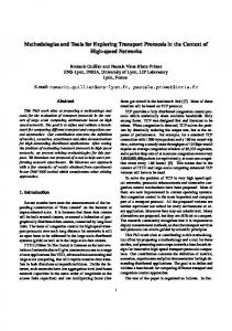
t FIG. 1 Illustration of the transport regimes: ballistic or more precisely quasi-ballistic regime (I), diffusive regime (II), and localized regime (III). For simplicity, no distinction is made for weak and strong localizations here. A zoom-in of the ballistic-to-diffusive transition is shown in the inset, where the ballistic limit, σ(E, t) = e2 ρ(E)vF2 (E)t, is indicated by the dashed line.

Figure 1 illustrates how the time-dependent conductivity evolves over time in a typical disordered lowdimensional material. In the limit of short time or length, electrons have not yet encountered any scatterers, and thus they propogate ballistically through the material. In this limit, the conductivity scales linearly with time, and this linear scaling can be used to extract the Fermi velocity vF (E), as shown in the inset of Fig. 1. At longer time or length scales, the electrons will be scattered by imperfections and will lose the memory of their previous momenta after a time of order of τp (E). This is equivalent to saying that after some time the VAC will decrease to zero, with a relation typically given by

9 (Beenakker and van Houten, 1991) Cvv (E, t) = vF2 (E)e−t/τp (E) .

(47)

Inserting this relation into Eq. (42) yields the semiclassical conductivity σsc (E) = e2 ρ(E)vF2 (E)τp (E),

(48)

which has the same form as that obtained from the Boltzmann transport formalism with the relaxation time approximation (Ashcroft and Mermin, 1976). The conductivity depends on the electronic structure through the DOS and the Fermi velocity, and on electron scattering through the momentum relaxation time. From the momentum relaxation time, one can define the mean free path as λ(E) = vF (E)τp (E).

(49)

In this limit the diffusion coefficient, or the diffusivity, is also well defined, D(E) = vF2 (E)τp (E).

(50)

From Eq. (48) one can see that the semiclassical conductivity is independent of time or length. Therefore, this diffusive limit of transport can be identified as the point when σ(E, t) saturates to a finite value, as indicated in the inset of Fig. 1. The ballistic-to-diffusive transition corresponds to an exponential decay of the VAC, or a quadratic-to-linear transition of the MSD. Finally, in the weak and strong localization regimes the conductivity is expected to decay with increasing system length (Lee and Ramakrishnan, 1985), as sketched in Fig. 1. The weak localization regime is characterized by a logarithmic decay of the conductivity, σ(E, L) − σsc (E) ∝ − ln(L/λ(E)), while the strong localization regime is associated with an exponential decay of the conductivity, σ(E, L) ∝ e−L/ξ(E) . Given that the electrons are localized within a given length of the order of ξ(E), the propagation length L(E, t) cannot evolve beyond this value. Therefore, the localization length can be determined from the time saturated value of the MSD (Triozon et al., 2000). Quantitatively, it is found that (Uppstu et al., 2014) ξ(E) = lim

t→∞

L(E, t) , 2π

(51)

where the localization length conforms with the standard definition in terms of the length scaling of conductance (Anderson et al., 1980). This relation is in accordance with the very original definition of Anderson localization (Anderson, 1958), namely, the absence of diffusion. III. LINEAR SCALING NUMERICAL TECHNIQUES

In Sec. II, we have presented three different representations of the Kubo formula for non-interacting electrons:

the Kubo-Greenwood formula in Eq. (22), the VAC-based Chester-Thellung formula in Eq. (42), and the MSDbased Roche-Mayou formula in Eq. (43). The aim of this section is to review the various numerical techniques for efficiently evaluating these formulas. For dissipative transport, we will show that the MSD-based formula is the most efficient and effective. For other nonequilibrium quantities such as Hall conductivity, spin susceptibility, and valley conductivity, the comparison between the different representations has just recently started, and the relative efficiency of different approximations is not yet entirely clear. However, the use of the kernel polynomial method to represent the Kubo-Bastin formula in Eq. (18) is possibly the most versatile approach (Garc´ıa et al., 2015). We will focus on dissipative transport in this section and discuss other transport properties in Sec. V. Our major concern in numerical implementations is the scaling of the computational cost with respect to the Hamiltonian size N . A common feature of the above Kubo formulas is that the trace can be evaluated using any complete set of single-particle wave functions that obey periodic boundary conditions (Chester and Thellung, 1959, 1961). One can use the eigenspace of the Hamiltonian, but this requires diagonalization, which is an O(N 3 ) process. This puts severe restrictions on the problem size to be treated. To enable the study of large systems (e.g., N > 106 ), a linear scaling, or O(N ) computation time is desirable. To achieve linear scaling, we avoid using the Hamiltonian’s eigenspace and instead work with a real-space tight-binding representation, where the basis functions are not eigenfunctions of the Hamiltonian but rather the electron orbitals around individual atoms. Because of this, the methods discussed in this review are usually referred to as real-space LSQT methods. Before discussing the relevant numerical techniques for achieving linear scaling, we list the quantities to be calculated for each implementation. A prominent quantity is the DOS defined in Eq. (27), which contains information about the electronic structure of the system. In the Kubo-Greenwood representation, one directly evaluates the electrical conductivity as given in Eq. (22). In the VAC representation of Eq. (42), one first calculates the product of the DOS and the VAC, h i 2 ˆ (t)Vˆ δ(E − H) ˆ U ˆ (t)† Vˆ , ρ(E)Cvv (E, t) = Re Tr U Ω (52) and then performs a numerical time integration to obtain the running electrical conductivity σ(E, t). In the MSD representation of Eq. (43), one first calculates the product of the DOS and the MSD, i 2 h ˆ X(t) ˆ − X) ˆ 2 , (53) ρ(E)∆X 2 (E, t) = Tr δ(E − H)( Ω and then performs a numerical time derivative to obtain the running electrical conductivity σ(E, t). In periodic

10 systems, it is problematic to use the absolute position ˆ We can change the above equation to an operator X. equivalent one (Triozon et al., 2004, 2002),

Each normalized random vector |φr i is constructed from N random coefficients,

i 2 ˆ U ˆ (t)]† δ(E − H)[ ˆ X, ˆ U ˆ (t)] . ρ(E)∆X 2 (E, t) = Tr [X, Ω (54) ˆ (t) using a polyAfter expanding the evolution operator U nomial of the Hamiltonian (as discussed below), the comˆ U ˆ (t)] only depends on the velocity operator mutator [X, (see Eq. (35)). This h is well i defined in periodic systems as ˆ ˆ the commutator X, H depends only on the difference

(58)

N 1 X |φr i = √ ξrn |ni . N n=1

h

in positions and not their absolute values, h i XX ˆ H ˆ = X, Hmn (Xm − Xn ) |mi hn| , m

(55)

n

where Xm is the position of the site associated with the mth orbital |mi and Hmn is the hopping integral between the mth and nth orbitals. There are some common features in these quantities: all the quantities are represented as a trace and involve ˆ and the time the quantum projection operator δ(E − H), ˆ (±t) appear in the VAC and MSD. evolution operators U Linear scaling techniques have been developed to evaluate these operators and we will discuss them in detail below. A. Evaluating the trace using a stochastic approach

Recall that the trace of an operator Aˆ is defined as X ˆ = Tr[A] hn| Aˆ |ni , (56)

Here, ξrn ∈ C are independent identically distributed random variables which have zero mean and unit variance. It has been shown that (Iitaka and Ebisuzaki, 2004; Weiße et al., 2006) √ the statistical error for the trace is proportional to 1/ Nr N , with the proportionality constant ˆ Usually, being related to the properties of the matrix A. a denser matrix gives a larger statistical error for a fixed value of Nr N . The statistical accuracy can be systematically improved by increasing Nr . In practice, for large N , a small Nr (on the order of 10) is sufficient to achieve a high statistical accuracy. Frequently used random vectors include random phase vectors (Drabold and Sankey, 1993; Iitaka and Ebisuzaki, 2004), where each coefficient ξrn is a phase factor eiθ with the phase variable θ uniformly distributed within [0, 2π); and random vectors with Gaussian distributed coefficients (Silver and Röder, 1994; Skilling, 1989). The actual choice of the distribution is not of particular importance (Weiße et al., 2006). For simplicity, we only use a single random vector |φi to present the subsequent formulas. In practice, one needs to check the convergence of the results with respect to Nr . Under the condition of sufficient average, in the following we use the “=” sign instead of the “≈” sign as in Eq. (57). We also use the normalization convention of hφ|φi = 1. Using this, we can express the quantities that need to be calculated as the following inner products:

n

ρ(E) =

{|ni}N n=1

where is a complete basis set of the problem, which is taken as a real-space tight-binding basis set in this review. The operator Aˆ relevant to this review will be essentially polynomials formed by the Hamiltonian and other quantities such as the velocity operator. What is important here is that even if Aˆ is highly sparse, such that the operation Aˆ |ni scales linearly, the total computation still has an O(N 2 ) scaling, which is better than O(N 3 ) for a non-sparse Aˆ but usually is still prohibitive. To achieve O(N ) scaling, the trace must be approximated. A powerful method for estimating the trace of large matrices is to use random vectors, a stochastic approach developed along with the methods of calculating spectral properties of large Hamiltonians (Drabold and Sankey, 1993; Silver and R¨ oder, 1994; Silver et al., 1996; Skilling, 1989; Weiße et al., 2006). In this stochastic method, one approximates the trace r by using Nr random vectors {|φr i}N r=1 , ˆ ≈ Tr[A]

Nr N X hφr | Aˆ |φr i . Nr r=1

(57)

σ(E) =

2N ˆ hφ|δ(E − H)|φi; Ω

2π~e2 N ˆ Vˆ δ(E − H) ˆ Vˆ |φi; hφ|δ(E − H) Ω

(59)

(60)

ρ(E)Cvv (E, t) =

h i 2N ˆ vac (t)i ; Re hφvac (t)|δ(E − H)|φ L R Ω (61)

ρ(E)∆X 2 (E, t) =

2N msd ˆ msd (t)i, (62) hφ (t)|δ(E − H)|φ R Ω L

where ˆˆ † |φvac L (t)i = V U (t) |φi;

ˆ †ˆ |φvac R (t)i = U (t) V |φi;

msd ˆ ˆ |φmsd L (t)i = |φR (t)i = [X, U (t)]|φi.

(63) (64)

The remaining task is to evaluate these inner products in a linear scaling way. We will discuss linear scaling numerical techniques related to the time evolution operˆ (t) in Sec. III.C and those related to the quantum ator U ˆ in Sec. III.D. Before doprojection operator δ(E − H) ing these, we first review a crucial numerical technique, namely the Chebyshev polynomial expansion.

11 B. Chebyshev polynomial expansion

We have presented different theoretical frameworks that can be used to determine the conductivity. We saw that a numerical evaluation of this quantity requires one to compute functions of the Hamiltonian matrix such as the time evolution operator and the quantum projection operator. We also discussed the need to choose an appropriate basis set so that the Hamiltonian can be represented as a sparse matrix. Therefore, if we want to exploit this feature, we need to find a way to avoid explicit evaluation of these quantities, because an arbitrary function of a sparse matrix is generally not a sparse matrix. The use of polynomial expansion provides a way to achieve the goal of linear scaling computation. Among various polynomials, the Chebyshev polynomials are usually the optimal choice (Boyd, 2001). The Chebyshev polynomials are a family of orthogonal polynomials which can be defined recursively. In this review we are using the Chebyshev polynomials of the first kind, {Tm (x)}, which are defined as Tm (cos(x)) = cos(mx) and have the recurrence relation T0 (x) = 1;

T1 (x) = x;

Tm (x) = 2x Tm−1 (x) − Tm−2 (x)

(m ≥ 2).

∞ X

f¯m Tm (x),

(66)

m=0

where f¯m =

2 1 + δm0

Z

1

−1

f (x)Tm (x) √ dx π 1 − x2

(67)

are the expansion coefficients and δm0 is the Kronecker delta. In general, one deals with functions of the Hamiltoˆ whose energy spectrum may exceed the internian H, val [−1, 1] in a particular unit system. In order to use the Chebyshev polynomial expansion, we must first scale ˆ such that the modified energy spectrum is and shift H in [−1, 1]. Specifically, this can be done by the linear transformation ˆ ¯ e = H −E, H ∆E

e = f (H)

X n

=

e |ni hn| = f (H)

∞ XX n m=0

=

∞ XX n m=0

=

∞ X

X n

en ) |ni hn| f (E

en ) |ni hn| f m Tm (E e |ni hn| f m Tm (H)

e f m Tm (H).

(69)

m=0

The inner products listed at the end of Sec. III.A are e |φR i. These quantities can thus of the form hφL | F (H) be evaluated iteratively by exploiting the recurrence relation of the Chebyshev polynomials and the whole computation breaks down to a number of sparse matrixvector multiplications, which scale linearly with the vector length N . In the next section, we discuss Chebyshev polynomial expansions of the time evolution operator and the regularized Green’s function.

(65)

These polynomials form a complete basis for functions defined on the real axis within the [−1, 1] interval. As such, they can be used to expand a function f (x) defined within the same interval in a polynomial series f (x) =

en } and eigenvectors {|ni}. For a general eigenvalues {E e we have function f (H),

(68)

¯ = (Emax +Emin )/2, where ∆E = (Emax −Emin )/2 and E with Emax and Emin being the maximum and minimum ˆ To avoid numerical problems, one usueigenvalues of H. ally makes ∆E slightly larger than (Emax −Emin )/2. Any e can thus be expanded in a manner simifunction of H e has the lar to Eq. (66). To see this, we assume that H

C. The time evolution operator and the regularized Green’s function

Both the VAC and MSD formalisms involve a time ˆ (t), which is absent from the Kuboevolution operator U ˆ Greenwood formula. The Dirac delta function δ(E − H) in the Kubo-Greenwood formula, on the other hand, is usually substituted by a regularized Green’s function (see Eq. (20)). In this subsection, we discuss the expansion of the time evolution operator and the regularized Green’s function in terms of the Chebyshev polynomials. In the VAC and MSD formalisms, after applying the random vector approximation for the trace, we only need to evaluate the application of the time evolution operator on a vector, as can be seen from Eqs. (63) and (64). Because we need information at a discrete set of time points, we need to construct an iterative scheme for evaluating the time evolution. The strategy is to divide the total correlation time into a number of steps. From time t to time t + ∆t (the time steps ∆t need not to be uniform), we have the following iterative relations for the vectors defined in Eqs. (63) and (64): ˆ † (t + ∆t)|φi = Vˆ U ˆ † (∆t)U ˆ † (t)|φi; Vˆ U

(70)

ˆ † (t + ∆t)Vˆ |φi = U ˆ † (∆t)U ˆ † (t)Vˆ |φi; U

(71)

ˆ U ˆ (t + ∆t)|φi = U ˆ (∆t)[X, ˆ U ˆ (t)]|φi [X, ˆ U ˆ (∆t)]U ˆ (t)|φi. + [X,

(72)

12 (a) 1.5 real-numerical imag-numerical cos(x t) -sin(x t)

U( t)

1 0.5 0

x=0.5;

t=100

-0.5 0

20

40

60

80

100

120

140

160

Np

(b) 4

10

3

numerical fit

Np

10

102

101 101

102

103

104

t

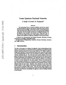
FIG. 2 Demonstration of the accuracy of the Chebyshev polynomial expansion of the time evolution operator using a simple function U (∆t) = exp(−ix∆t). (a) The real part cos(x∆t) and the imaginary part − sin(x∆t) of U (∆t), calculated analytically (dashed lines) or by a numerical expansion (markers) similar to that in Eq. (73). Here, x plays the role of the Hamiltonian in the time evolution operator and we choose x = 0.5 and ∆t = 100. (b) The number of Chebyshev polynomials Np required for achieving a precision of 10−15 as a function of the time interval ∆t. In the large ∆t limit, Np ∝ ∆t, as indicated by the dashed line.

Therefore, the task further breaks down to evaluating the ˆ (±∆t) and [X, ˆ U ˆ (∆t)] on application of the operators U some vectors. The Chebyshev polynomial expansion is particularly efficient when the expanded function is regular and differentiable. One of its first uses was the expansion of the ˆ (±∆t). Solving the integral in time evolution operator U Eq. (67) for this operator leads to an expansion in the form of Eq. (69) (Tal-Ezer and Kosloff, 1984), Np

ˆ (±∆t) ≈ U

X

e U m (±∆t)Tm (H),

(73)

m=0

U m (±∆t) = (2 − δm0 )(∓i)m Jm (ω0 ∆t) ,

(74)

where ω0 ≡ ∆E/~ and Jm (x) is the mth order Bessel function of first kind. This is probably one of the earliest uses of the Chebyshev polynomial expansion in quantum physics. The Chebyshev polynomial expansion of

the time evolution operator can be evaluated up to machine precision and the order of expansion Np needed for achieving this is linearly proportional to the time interval in the limit of large ∆t. When m is increased to a critical value, the Bessel function Jm (ω0 ∆t) suddenly decays to zero and the expansion suddenly approaches the exact value. An illustration of this fast convergence can be seen in Fig. 2, for the simple function U (∆t) = exp(−ix∆t). It has been shown that the Chebyshev polynomial expansion approach is more than two orders of magnitude more efficient than a naive Taylor expansion approach (Markussen, 2006). A comparison between a few widelyused time propagation algorithms for the time-dependent Schrödinger equation revealed that the Chebyshev polynomial expansion approach is the optimal choice for timeindependent potentials (Leforestier et al., 1991). The Chebyshev polynomial expansion approach has also been demonstrated to be very efficient and reliable for determining the quantum dynamics of complex many-particle systems (Fehske et al., 2009). ˆ U ˆ (∆t)] can be similarly expanded in The operator [X, terms of the Chebyshev polynomials,

ˆ U ˆ (∆t)] ≈ [X,

Np X

e (2 − δm0 )(−i)m Jm (ω0 ∆t) [X, Tm (H)],

m=0

(75) e can be calculated itwhere the commutator [X, Tm (H)] eratively using the following recurrence relation:

ˆ Tm (H)] e = 2[X, ˆ H]T e m−1 (H) e + 2H[ e X, ˆ Tm−1 (H)] e [X, ˆ Tm−2 (H)]. e − [X, (76)

Algorithms 1 and 2 give explicit steps for evaluating ˆ (±∆t)|φin i and |φout i = [X, ˆ U ˆ (∆t)]|φin i. |φout i = U

ˆ (±∆t)|φin i Algorithm 1 Evaluating |φout i = U 1: |φ0 i ← |φin i 2: 3: 4: 5: 6: 7: 8: 9: 10: 11:

e in i |φ1 i ← H|φ |φout i ← J0 (ω0 ∆t) |φ0 i + 2(∓i)J1 (ω0 ∆t) |φ1 i m←2 while abs [Jm (ω0 ∆t)] > 10−15 do e 1 i − |φ0 i |φ2 i ← 2H|φ |φout i ← |φout i + 2(∓i)m Jm (ω0 ∆t) |φ2 i |φ0 i ← |φ1 i |φ1 i ← |φ2 i m←m+1 end while

13 ˆ U ˆ (∆t)]|φin i Algorithm 2 Evaluating |φout i = [X,

2006). These coefficients, in contrast to those for the time evolution operator, do not decay but oscillate with increasing m. This is the reason for the presence of η, which provides a damping of the coefficients and improves the convergence of the expansion. It has been argued that approximating the Green’s function in this way may actually be incorrect because of the lack of positiveness of the approximation (Weiße et al., 2006), which could lead to an incorrect position of the pole of the Green’s function. Nonetheless, we believe that this should not be the case as long as the number of moments is large enough. In the next subsection, we discuss different approaches to deal with singular functions in the context of approximating the quantum projection operator.

1: |φ0 i ← |φin i 2: |φx 0i ← 0

e 0i 3: |φ1 i ← H|φ 4: 5: 6: 7: 8: 9: 10: 11: 12: 13: 14: 15: 16:

ˆ H]|φ e 0i |φx1 i ← [X, |φout i ← 2(−i)J1 (ω0 ∆t) |φx1 i m←2 while abs [Jm (ω0 ∆t)] > 10−15 do e 1 i − |φ0 i |φ2 i ← 2H|φ ˆ H]|φ e 1 i + 2H|φ e x1 i − |φx0 i |φx2 i ← 2[X, m |φout i ← |φout i + 2(−i) Jm (ω0 ∆t) |φx2 i |φ0 i ← |φ1 i |φ1 i ← |φ2 i |φx0 i ← |φx1 i |φx1 i ← |φx2 i m←m+1 end while

++ The Green’s function is a spectral quantity that can also be evaluated using the Chebyshev polynomial expansion, although it has a singularity which carries physical information of the system, and therefore should be treated with special care. In Sec. II we introduced the η parameter, which is a consequence of an adiabatic switching on of the electric field. This parameter broadens the singularity of the Green’s function, serving effectively as a mathematical regularization which enables one to approximate the Green’s function using a Chebyshev polynomial expansion. This procedure was done first by Vijay et al. (Vijay et al., 2004) in the context of spectral filters, and was later applied by Ferreira and Mucciolo to quantum transport, where it was dubbed the Chebyshev-polynomial Green’s function (CPGF) method (Ferreira and Mucciolo, 2015). Applying the Chebyshev coefficients of the time evolution operator, cf. Eq. (74), to the integrand of the time domain representation of the Green’s function in Eq. (19), and using a Laplace transform of the Bessel function (Gradshteyn and Ryzhik, 1975), we get the following Chebyshev polynomial expansion for the advanced Green’s function: G+ (E) =

1 X e gm (z)Tm (H); ∆E m

−1

gm (z) = (2 − δm0 )i

√ m z − i 1 − z2 √ , 1 − z2

(77)

(78)

e + ie where z = E η and ηe = η/∆E. In the limit of η = 0, it is easy to see that the Chebyshev coefficients reduce to h i e exp −i m arccos(E) e = (2 − δm0 )i−1 p gm (E) . (79) e2 1−E This expression has been obtained by several authors (Covaci et al., 2010; Garc´ıa et al., 2015; Weiße et al.,

D. Evaluating the quantum projection operator

We now turn to discuss the evaluation of the quanˆ involved in all the tum projection operator δ(E − H) conductivity formulas. There are several linear scaling techniques for approximating this operator, including the Lanczos recursion method (LRM) (Dagotto, 1994; Haydock et al., 1972, 1975; Haydock, 1980; Petitfor and Weaire, 1985), the Fourier transform method (FTM) (Alben et al., 1975; Feit et al., 1982; Hams and De Raedt, 2000), the kernel polynomial method (KPM) (Silver and Röder, 1994; Silver et al., 1996; Wang, 1994; Wang and Zunger, 1994; Weiße et al., 2006), and the maximum entropy method (MEM) (Drabold and Sankey, 1993; Silver and Röder, 1997; Skilling, 1989). We will only review the first three methods (LRM, FTM, and KPM), as the last one (MEM) has not been used in LSQT calculations. A comparison between the MEM and the KPM can be found in a previous review (Weiße et al., 2006). In the context of LSQT calculations, the LRM is the most widely used one, the FTM has only been used in one group (Yuan et al., 2010a,b; Zhao et al., 2015), and the KPM has been recently used in different groups on various problems (Cummings et al., 2017; Fan et al., 2014a; Garc´ıa et al., 2015) and has started to gain popularity. Although we have a few different quantities to calculate, it suffices to discuss these methods in terms of the DOS as given in Eq. (59). Generalizations to other quantities are straightforward.

1. The Lanczos recursion method

The LRM is based on the Lanczos algorithm (Lanczos, 1950) for tridiagonalizing sparse Hermitian matrices. The Lanczos algorithm is usually used to obtain extremal eigenvalues and the corresponding eigenstates (Cullum and Willoughby, 1985), but it can also be used to calculate spectral properties (Haydock et al., 1972,

14 1975; Haydock, 1980; Petitfor and Weaire, 1985). The first step of the LRM is to project the Hamiltonian onto an orthogonal basis in a Krylov subspace, generating a tridiagonal matrix (a matrix that has nonzero elements only on the main diagonal and the first diagonals below and above the main diagonal)   a1 b2 0 ··· 0   ..  b2 a2 . b3 0      .. (80) T =  0 ... ... . . 0    . .   .. . . bM −1 aM −1 bM  0 ··· 0 bM aM The dimension M of the tridiagonal matrix can be much smaller than the dimension N of the original matrix. The matrix elements {an } and {bn } are obtained from a Lanczos algorithm. There are multiple versions of the Lanczos algorithm and the most numerically stable one is given in Algorithm 3 (Saad, 2003). The computational effort of the LRM is thus proportional to N M , which is O(N ) when M N . Algorithm 3 Lanczos algorithm (Saad, 2003)

E + iη − a1 −

b22 E+iη−a2 −···

.

The FTM is very simple conceptually: it is based on the Fourier transform of the Dirac δ function as given by Eq. (23). Ideally, the time integral is over the whole real axis, but in practice, one can only reach a finite time with a finite time step ∆τ . Therefore, one should be satisfied with a truncated and discrete Fourier transform, M ∆τ X i(E−H)m∆τ ˆ /~ ˆ e . δ(E − H) ≈ 2π~

(82)

m=−M

where M ∆τ represents the upper limit of the time integral in Eq. (23). Using the discrete Fourier transform, we can write the DOS in Eq. (59) as

The second step of the LRM is to calculate the first element of the advanced Green’s function G+ (E) = ˆ −1 in the Lanczos bases {|φm i} using the (E + iη − H) continued fraction 1

2. The Fourier transform method

A direct expansion in this way leads to Gibbs oscillations, and window function is usually used to suppress them. A frequently used one is the Hann window πm 1 1 + cos , (83) wm = 2 M +1

Require: |φ1 i = |φi is the normalized random vector 1: b1 ← 0 2: |φ0 i ← 0 3: for m = 1 to M do 4: |ψm i ← H|φm i − bm |φm−1 i 5: am ← hψm |φm i 6: |ψm i ← |ψ pm i − am |φm i 7: bm+1 ← hψm |ψm i 8: |φm+1 i ← |ψm i/bm+1 9: end for

hφ|G+ (E)|φi =

iη in the Green’s function, i.e., δE = η. One should therefore make sure that a sufficiently large M is used to ensure converged results. However, it is well known that in its basic forms such as that presented in Algorithm 3, the Lanczos algorithm can become numerically unstable when M is large, due to the loss of orthogonality in the Lanczos basis vectors. The Lanczos basis vectors can be explicitly orthogonalized (Saad, 2003), but this will increase the computational complexity of the algorithm, making it less efficient than other methods.

(81)

The DOS of Eq. (59) can then be calculated using the relation between the quantum projection operator and the Green’s function given in Eq. (20). The computation time for the second step is proportional to M Ne , where Ne is the number of energy points considered in the calculation. Usually, Ne N , and the computation time for the second step is thus negligible compared to the first step. Because of this, the overall computational effort almost does not scale with respect to Ne . We can say that the algorithm is parallel in energy, which is a common feature for all the methods presented below. An important issue is the energy resolution δE achievable using a given number of recursion steps M . The energy resolution is actually set by the imaginary energy

∆τ N ρ(E) ≈ π~Ω

M X

eiEm∆τ /~ wm Fm ,

(84)

ˆ ˆ (m∆τ )|φi Fm = hφ|e−iHm∆τ /~ |φi = hφ|U

(85)

m=−M

where

is the mth Fourier moment. Based on the formulas above, we can see that the FTM consists of the following two steps: (1) construct a set of Fourier moments {Fm } as defined in Eq. (85), and (2) calculate physical properties such as the DOS from the Fourier moments through a discrete Fourier transform as given by Eq. (84). Similar to the case of the LRM, the computation time for the second step is negligible compared to the first one and the algorithm is essentially parallel in energy. As the Fourier moments are the expectation values of the time evolution operator, this method is also usually called the equation of motion method (Alben et al., 1975) or the time-dependent Schrödinger equation method (Feit et al., 1982; Hams and De Raedt,

15 2000). Note that we have used ∆τ here to distinguish it from the correlation time step ∆t in the VAC and MSD formalisms. Based on the Nyquist sampling theorem, which states that the sampling rate must be no less than the Nyquist rate 2fmax to perfectly reconstruct a signal with spectrum between 0 and fmax , the optimal value of ∆τ can be determined to be ∆τ = π~/∆E, giving ω0 ∆τ = π. Using this ∆τ , the energy resolution is given by δE ∼ ∆E/M (Feit et al., 1982).

fn } are the eigenvalues of the scaled Hamiltowhere {E nian. A general term in the sum can be expanded in the form of Eq. (86) as

3. The kernel polynomial method

and Eq. (69), we obtain a Chebyshev polynomial expansion for the DOS in Eq. (59),

In Sec. III.B we introduced the Chebyshev polynomial expansion as a useful tool for approximating regular functions and discussed additionally the problem of expanding a singular function such as the Green’s function using the so-called CPGF method (Ferreira and Mucciolo, 2015). There, the singularity in the Green’s function was regularized by introducing a small imaginary energy iη. There is another widely used approach to handle the singularity in the function to be expanded in terms of Chebyshev polynomials, which is called the kernel polynomial method (KPM) (Silver and R¨ oder, 1994; Silver et al., 1996; Wang, 1994; Wang and Zunger, 1994; Weiße et al., 2006). In this method, the Gibbs oscillations near the points where the expanded function f (x) is not continuously differentiable are damped by multiplying the Chebyshev coefficients with a damping factor gm . This is equivalent to convolving the function with a kernel K(x) (Silver et al., 1996; Weiße et al., 2006). Each kernel corresponds to a damping factor. Here, it is more convenient to rewrite the Chebyshev polynomial expansion in the following way (Silver et al., 1996; Weiße et al., 2006): ∞ X 1 (2 − δm0 )cm Tm (x), f (x) = π 1 − x2 m=0

√

(86)

where Z

∞ X 1 fn )Tm (E). e p (2 − δm0 )Tm (E e 2 m=0 π 1−E (90) Using the property of the δ function,

e−E fn ) = δ(E

ˆ = δ(E e − H)/∆E, e δ(E − H)

∞ X 2N DOS e p (2 − δm0 )Cm ρ(E) = Tm (E), e 2 m=0 πΩ∆E 1 − E (92) where DOS e Cm = hφ|Tm (H)|φi

dxf (x)Tm (x).

M X 2N DOS e p (2 − δm0 )gm Cm Tm (E). ρ(E) = e 2 m=0 πΩ∆E 1 − E (94) The optimal kernel varies with the specific application. For the expansion of the quantum resolution operator, which is essentially a set of delta peaks, the Jackson kernel with the following damping factor (α = 1/(M + 1)) J gm = (1 − mα) cos (πmα) + α sin (πmα) cot (πα) (95)

has been found to be optimal (Silver et al., 1996; Weiße et al., 2006), as it produces the smallest broadening. If one considers the Green’s function, the Lorentz kernel with the damping factor L gm (λ) =

(87)

−1

The essence of the KPM is to truncate the infinite series to a finite order M and multiply the expansion coefficient cm by a damping factor gm , f (x) ≈

M X 1 (2 − δm0 )gm cm Tm (x). π 1 − x2 m=0

√

(88)

We now derive an expression of the DOS in the KPM. We start with the identity e − H)] e = Tr[δ(E

X n

e−E fn ), δ(E

(89)

(93)

are the Chebyshev moments for the DOS. Truncating to a finite number of Chebyshev moments and introducing the damping factors, we find

+1

cm =

(91)

sinh[λ(1 − m/M )] sinh(λ)

(96)

may offer a better choice (λ is a parameter which is usually chosen to be 3-5). In Fig. 3 we plot the Jackson and Lorentz damping factors along with the Hann window function, where the expansion order is chosen as M = 104 . To demonstrate the performance of the different damping factors and the window function, we use them to approximate the simple δ function δ(x) = δ(x − 0). The Chebyshev expansion in the KPM can be written as δ(x) =

M X 1 (2 − δm0 )gm Tm (0)Tm (x). π 1 − x2 m=0

√

(97)

16

Damping factor or window function

1 Hann Jackson Lorentz

0.8

0.6

0.4

0.2

0 0

2000

4000

6000

8000

10000

m

FIG. 3 Comparison between different damping factors and a J window function, including the Jackson damping factor gm L defined in Eq. (95), the Lorentz damping factor gm (λ = 4) defined in Eq. (96), and the Hann window function wm defined in Eq. (83).

3: 4: 5: 6: 7: 8: 9: 10:

FTM-Hann KPM-Jackson KPM-Lorentz CPGF

1500

(x)

1000

500

0

-1.5

-1

-0.5

0

x

0.5

1

1.5

2 10-3

FIG. 4 Approximation of the single-variable function δ(x) J using the KPM with the Jackson damping gm defined in Eq. L (95), the Lorentz damping gm (λ = 4) defined in Eq. (96), the CPGF method, and the FTM with the Hann window wm defined in Eq. (83). Here, M = 104 for the KMP and M = 2000 for the FTM. Note that the x and y axes differ by a factor of 106 in magnitude.

The results obtained by using the KPM with different damping factors are shown in Fig. 4. Also shown are the results obtained by using the Fourier expansion, δ(x) =

Algorithm 4 Evaluating the Chebyshev moments e Ri hφL |Tm (H)|φ 1: |φ0 i ← |φR i 2: C0 ← hφL |φ0 i

2000

-500 -2

and the CPGF method (Ferreira and Mucciolo, 2015). With the same value of M = 104 , the Jackson damping gives a narrower shape compared to the Lorentz damping and therefore has a finner resolution, while the CPGF method is essentially equivalent to the KPM with the Lorentz damping (λ = 4) when the resolution parameter in the CPGF method is chosen as 4/M . We also note that while the Gibbs oscillations can be effectively suppressed using the KPM, they persist in the case of the FTM. Apart from being less effective in suppressing Gibbs oscillations, the FTM has also been shown to be less computationally efficient as compared to the KPM (Fan et al., 2014a). This comparison and the comparison between the KPM and the LRM (Silver et al., 1996; Weiße et al., 2006) indicate that the KMP with the Jackson damping factor is the optimal approach for approxiˆ which mating the quantum projection operator δ(E − H), essentially consists of a set of δ peaks.

M M X 1 X 2 − δm0 wm eiπmx = wm cos(πmx), 2 2 m=0 m=−M

(98)

e 0i |φ1 i ← H|φ C1 ← hφL |φ1 i for m = 2 to M do e 1 i − |φ0 i |φ2 i ← 2H|φ Cm ← hφL |φ2 i |φ0 i ← |φ1 i |φ1 i ← |φ2 i end for

We can now summarize the procedure of the KPM: (1) construct a set of Chebyshev moments {Cm } (see Algorithm 4), and (2) calculate physical properties such as the DOS from the Chebyshev moments through a finiteorder Chebyshev polynomial summation as given by Eq. (94). Similar to the case of the LRM and the FTM, the construction of the Chebyshev moments dominates the computation time and the algorithm is parallel in energy. The energy resolution achieved in the KPM is δE ∼ ∆E/M (Weiße et al., 2006), similar to the case of the FTM. E. Physics of the regularization of Green’s function

We have seen previously that seemingly different results can be obtained depending on what approximation is chosen to represent the Green’s functions. In this sense, one may wonder if one approximation is better than the other, or if there are any criteria for choosing a specific one. It turns out that each approximation represents a specific physical situation, and therefore, this should the criterion for choosing a particular one. If one considers the DC Kubo formula in Eq. (7), one interesting feature is the limit η → 0, which represents

17 the adiabatic process of turning the electric field on. In linear response theory, the electric field is not included specifically in the Hamiltonian, but enters as an external perturbation to the system. Therefore, one can think ˆ as describing an open system in of the Hamiltonian H contact with a reservoir which induces an electric field. Within the linear response limit, the dynamics of the system, driven out of equilibrium by this external field, will be mainly described by its intrinsic properties. The proper adiabatic limit implies that the process occurs slowly enough for the electrons to respond instantaneously to the change, dominating all other relevant timescales. The diffusive behavior in metals is for instance determined by the momentum relaxation time τp , so in order to simulate correctly the transport behavior one needs η < ~/τp . When one aims at describing spin-related phenomena, quantities such as the spin relaxation rate and the spin precession frequency also need to be compared with η. Finally, simulations are performed in systems with a finite number of atoms, which sets a minimal energy scale associated with the energy level spacing δE. Given that the goal is to simulate effectively infinite systems, one must meet the condition δE < η while also satisfying δE, η “physically relevant energy scales” in order to capture the relevant physics of the system being simulated. This discussion will be helpful to understand the different results and the different approximations performed numerically.

F. Numerical examples

Here, we use some numerical examples to illustrate the formalisms and techniques discussed above. We use the Anderson model (Anderson, 1958) to illustrate the numerical techniques. We consider the nearest-neighbor tight-binding model defined on a square lattice with lattice constant a and dimension N = Nx ×Ny . The Hamiltonian can be written as X X H= (−γ)c†i cj + Ui c†i ci , (99) ij

i

where −γ is the hopping integral and Ui are the onsite potentials. The on-site potentials are uniformly distributed in an interval [−W/2, W/2], where W is called the Anderson disorder strength. For simplicity, we consider open boundary conditions in the y direction and study the transport in the x direction.

1. Formalisms to be compared

We compare three representations of the Kubo conductivity, including the VAC representation of Eq. (42), the

MSD representation of Eq. (43), and the KG representation of Eq. (22). For the VAC and MSD representations, we use the KPM for the quantum projection operator. The quantity to be calculated in the VAC representation is the product of the DOS and the VAC M

X 2N p (2 − δm0 ) e 2 m=0 πΩ∆E 1 − E e vac (t), × gm Tm (E)C (100)

ρ(E)Cvv (E, t) =

m

where h i vac e vac Cm (t) = Re hφvac L (t)|Tm (H)|φR (t)i

(101)

are the Chebyshev moments of ρ(E)Cvv (E, t). The quantity to be calculated in the MSD representation is the product of the DOS and the MSD M X 2N p (2 − δm0 ) e 2 m=0 πΩ∆E 1 − E e msd (t), × gm Tm (E)C (102)

ρ(E)∆X 2 (E, t) =

m

where msd e msd Cm (t) = hφmsd L (t)|Tm (H)|φR (t)i

(103)

are the Chebyshev moments of ρ(E)∆X 2 (E, t). We call these the VAC-KPM and MSD-KPM methods. For the Kubo-Greenwood formalism, we consider a numerical implementation based on the Chebyshev polynomial expansion of the Green’s function according to Eq. (77), which we call the KG-CPGF method (Ferreira and Mucciolo, 2015). In this method, one first writes the KuboGreenwood conductivity Eq. (60) as 2~e2 N hφ| V Im[G+ (E)]V Im[G+ (E)] |φi . πΩ (104) Here, we have highlighted the η-dependence of the conductivity. Then, using the Chebyshev expansion of the Green’s function in Eq. (77), we have σ(E, η) =

M M 2~e2 N X X kg Im[gm (z)]Im[gn (z)]Cmn πΩ(∆E)2 m=0 n=0 (105) where gm (z) is given in Eq. (78) and

σ(E, η) =

kg e Tn (H) e |φi . Cmn = hφ| V Tm (H)V

(106)

The LSQT methods to be compared are listed in Table I. In addition to algorithmic improvements, increasing computing power has played an important role in advancing quantum transport simulations. In massively parallel computing, the use of graphics processing units

18 TABLE I Summary of the different LSQT approaches for calculating the dissipative conductivity. The computational cost is measured in terms of the number of matrix-vector multiplications. Here, M is the order of the Chebyshev polynomial expansion for the quantum projection operator or the Green’s function, and tmax is the maximum correlation time in the VAC and MSD formalisms. The whole time block [0, tmax ] is divided into Nt intervals, which are not necessarily uniform. LSQT method Explicit formulas Applicability to ballistic regime Applicability to diffusive regime Applicability to localized regime Computational cost

VAC-KPM MSD-KPM KG-CPGF Eqs. (42),(100) and (101) Eqs. (43),(102) and (103) Eqs. (105) and (106) Yes Yes No Yes Yes Yes but slow Not practical Yes Not quantitatively ∼ M Nt + 10ω0 tmax ∼ M Nt + 10ω0 tmax ∼ M2

(GPUs) is playing a more important role in various simulation methods used in computational physics (Harju et al., 2013). It turns out that the linear scaling techniques perform particularly well on GPUs (Fan et al., 2014a; Garc´ıa et al., 2015). Note that the LSQT calculations shown in this subsection have been actually obtained using an open source code named GPUQT (Fan et al., 2018), which is fully implemented on GPUs. A Matlab implementation of pedagogical value is also publicly available (Fan, 2018a). We will also closely compare the above LSQT methods with the Landauer-B¨ uttiker (LB) method (Datta, 1995; Ferry and Goodnick, 1997), which we briefly introduce here. In tight binding calculations, the recursive Green’s function formalism (Lewenkopf and Mucciolo, 2013) is usually used. Our LB calculations here were performed using a publicly available code (Fan, 2018b). In the LB approach, the contacts are modeled as ballistic semi-infinite leads and the conductance g(E) is obtained from the transmission function T (E), g(E) =

2e2 T (E). h

(107)

For a single mode system, the transmission function equals the probability of a charge carrier to transmit from one contact to another. If there are several transport modes involved, the transmission function equals the sum of the transmission probabilities for the different modes. There are many equivalent forms for the transmission function, and here we adopt the Caroli (Caroli et al., 1971) form, T (E) = Tr[G(E)ΓL G† (E)ΓR ],

(108)

where G(E) is the retarded Green’s function of the device, G† (E) is the advanced Green’s function, and ΓL and ΓR describe the coupling of the device to the leads. The retarded Green’s function for a system attached to two leads is G(E) =

1 ˆ − ΣL (EL ) − ΣR (ER ) E−H

,

(109)

where ΣL (EL ) is the self energy of the left lead at Fermi energy EL and ΣR (ER ) is the self energy of the right lead at Fermi energy ER . The Fermi energies EL and ER of the leads can be set to the same value as in the device, E, or to an arbitrary value. In the calculations below, we set EL = ER = E. The self energy matrices can be obtained through different methods, e.g., using an iterative method (Sancho et al., 1985). The coupling matrices ΓL and ΓR are the imaginary part of the self energies, ΓL/R = i ΣL/R − Σ†L/R = −2Im ΣL/R . (110) 2. Ballistic regime

As discussed in Sec. II.C.3, the VAC and MSD formalisms capture the essential physics of ballistic transport. To illustrate this, we consider a narrow ribbon with Ny = 2 and free boundary conditions in the transverse direction. To achieve high accuracy in the random vector approximation, we set Nx = 5 × 106 in the transport direction and average the results over Nr = 10 random vectors. The total number of tight binding orbitals is thus N = 107 . We use the KPM with M = 3000. The VAC at the band center E = 0 is a constant, vF2 = 3, as shown in Fig. 5(a). Consequently, the MSD in Fig. 5(b) is a quadratic function of the correlation time, ∆X 2 (E, t) = vF2 (E)2 t2 . In other words, the electrons are propagating at a constant velocity without scattering. The DOS ρ(E) and the group velocity vF (E) are shown in Figs. 5(c) and (d). From these, we can calculate the ballistic conductance as g(E) = e2 ρ(E)vF (E)/2, as given by the solid line in Fig. 6. For comparison, we also show the conductance calculated using the LB method, which is represented by the dashed line. Remarkably, the VAC-KPM and MSD-KPM methods produce the correct conductance plateaus. Around the band edges, however, these methods overshoot the conductance plateau, as has been noticed in a variety of studies (Charlier et al., 2007; Fan et al., 2014a; Markussen et al., 2006). When the system contains some disorder, deviating the conduction

19 (a)

(b)

4

(a)

300

(b) 1.5

1500

3 200

1 1000

2 100

0.5

0

0

1 500

0 0

2

4

6

8

10

0

2

4

6

8

10 -0.5

(d)

(c)

0 0

2

3

20

40

60

(c)

1.5

0

20

40

60

(d) 40

2

60

1 30

1 0.5

40

0 -5

0

20

0 -4

5

-2

0

2

VAC-KPM MSD-KPM KG-CPGF

4 10

FIG. 5 Electronic and transport properties of a disorder-free square lattice ribbon with width Ny = 2. (a) VAC and (b) MSD at E = 0 as a function of correlation time. (c) DOS and (d) group velocity as a function of Fermi energy.

10 VAC-KPM (MSD-KPM) LB

8

6

20

0 0

30

60

90

120

150

VAC-KPM MSD-KPM KG-CPGF LB

0 -5 -4 -3 -2 -1 0 1 2 3 4 5

FIG. 7 Results for the E = 0 energy point in a square lattice with Ny = 50 and W = γ. (a) VAC, (b) MSD, and (c) running electrical conductivity as a function of time t. For the VAC-KPM and MSD-KPM methods, t refers to the correlation time; for the KG-CPGF method, t refers to the inverse energy resolution ~/η. (d) Semiclassical conductivity σsc as a function of energy E from the various methods. Because the LB method is not parallel in energy, only a few energy points were considered.

3. Diffusive regime

4

2

0 -5

-4

-3

-2

-1

0

1

2

3

4

5

FIG. 6 Ballistic conductance in a disorder-free square lattice ribbon with width Ny = 2 obtained using the VAC-KPM (or equivalently MSD-KPM) method (solid line) and the LB method (dashed line).

regime from purely ballistic motion, the MSD formalism becomes extremely suitable for calculating lengthdependent conductance, as largely illustrated in applications to carbon nanotubes (Charlier et al., 2007; Roche and Saito, 2001; Roche et al., 2001).

We next consider a disordered system and closely compare the different LSQT methods as well as the LB method in the ballistic-to-diffusive crossover regime. As a generic case, we take a square lattice with width Ny = 50 and for an Anderson disorder strength W = γ. In the LSQT calculations, Nx = 2 × 105 , Nr = 10, and M = 3000. In the LB method, we increase the system length from L = a to 100a and calculate the conductance g(E, L) iteratively. We average over 100 disorder realizations in the LB calculations. Results for the E = 0 energy point are shown in Fig. 7. As expected, the VAC decays exponentially with increasing correlation time [Fig. 7(a)] and the MSD changes from a quadratic to a linear function of correlation time [Fig. 7(b)]. The running electrical conductivities calculated from the VAC (via a time integration) and the MSD (via a time derivative) are totally equivalent, as can be seen in Fig. 7(c). While the meaning of time is clear in the VAC and the MSD formalisms, it is ambiguous in the KG-CPGF method. It has been suggested (Ferreira and Mucciolo, 2015) that one can regard the inverse of the energy resolution ~/η as the timescale of the problem. Figure 7(c)

20 shows the evolution of the electrical conductivity with respect to this time variable, which is clearly inequivalent to the correlation time in the VAC and MSD formalisms. The electrical conductivity reaches the maximum diffusive value within t = 30~/γ in the VAC and MSD formalisms. In contrast, the electrical conductivity is not converged up to the maximum time of ~/η = 150~/γ associated with the highest energy resolution permitted by the number of Chebyshev moments M = 3000 in the KG-CPGF method. Because the system will eventually enter the localized regime, there must be a maximum value of the scale-dependent electrical conductivity, which can be defined as the semiclassical conductivity σsc (E). This is the conductivity attained in the system before coherent backscattering and quantum interferences come into play. In the VAC and MSD formalisms, this maximum conductivity can be obtained straightforwardly. In the KG-CPGF method, however, one needs to make an extrapolation whenever the running quantum conductivity is not yet converged. Figure 7(d) shows that the semiclassical conductivity σsc (E) obtained from the various methods are equivalent to each other. In the LB method, we calculate the semiclassical conductivity based on the ballistic-to-diffusive formula (Datta, 1995) 1 L 1 1 = + , g(E, L) σsc (E) Ny a g0 (E)

(111)

where g0 (E) is the ballistic conductance at energy E. Although the KG-CPGF method gives consistent results for the semiclassical conductivity as compared to the VAC and MSD formalisms, it is obviously much less efficient and can lead to misleading interpretations. Here, we quantitatively analyze the computational complexities of these methods. Because the major calculations are matrix-vector multiplications (MVMs), we quantify the computational cost in terms of the number of MVMs. In the MSD-KPM method, the evaluations of the time evolution and the quantum projection operator are decoupled. According to Fig. 2(b), it takes about αω0 tmax iterations to evaluate the time evolution operator [X, U (tmax )], where tmax is the maximum correlation time and α is a numerical factor of the order of 1. According to Algorithm 2, the number of MVMs for each iteration is 3 and the number of MVMs for the time evolution part is thus 3αω0 tmax . As a conservative estimate we round this number up to 10ω0 tmax . According to Algorithm 4, the number of MVMs for evaluating the quantum projection operator using the KPM is M Nt , where Nt is the number of time intervals. The total computational cost in the MSD-KPM method is thus M Nt + 10ω0 tmax . The computational cost in the VACKPM method can be determined to be the same. In the KG-CPGF method, there is no explicit time evolution, and the computational cost is M 2 , scaling quadratically with respect to M .

In this example, we have considered a total correlation time of tmax = 60~/γ with Nt = 30 intervals. Because we set ∆E = 5γ in this example, we have ω0 tmax = 300. The computational cost in the MSD-KPM and VACKPM methods is thus M Nt + 10ω0 tmax = 93000. In contrast, the computational cost in the KG-CPGF method is M 2 = 9 × 106 , which is two orders of magnitude higher than that in the MSD-KPM and VAC-KPM methods. The high computational cost of the KG-CPGF method severely limits its applications in weakly disordered systems, where long time evolution is required to reach the diffusive regime and one has to consider a large value of M. 4. Localized regime

It is well known that electrons are localized in the Anderson model (Anderson, 1958). In this example, we consider a square lattice with the same width Ny = 50 as in the last example, but with a larger disorder strength W = 5γ. 10 1 MSD-KPM KG-CPGF LB 2

10 0

10 -1

10 -2

10 -3 0

100

200

300

400

FIG. 8 Conductance g at E = 0 as a function of length L. In the MSD-KPM method, L is calculated using Eq. (44). In the KG-CPGF method, L is calculated using Eq. (112). The vertical dashed line indicates the length 2πξ up to which the propagating length L(E, t) in the MSD formalism can reach.

In the LSQT calculations (including the MSD-KPM and KG-CPGF methods), Nx = 2 × 105 , Nr = 10, and M = 3000. We convert the conductivity to conductance using Eq. (45). In the MSD formalism, L is calculated using Eq. (44). In the CPGF formalism, L is calculated using (Ferreira and Mucciolo, 2015) L(E, η) = πv(E)~/η.

(112)

In the LB method, we average over 5000 disorder realizations to obtain the typical conductance (Anderson et al.,

21 1980) gtyp (E, L) = exp[hln g(E, L)i].

(113)

Figure 8 shows the conductances at E = 0 calculated using the three methods. As expected, the conductance decays exponentially in the large length limit in the LB formalism. This provides a definition of the localization length ξ(E), gtyp (E, L) ∼ exp[−L/ξ(E)].

(114)

The localization length at E = 0 is fitted to be ξ ≈ 16a. The conductance calculated from the MSD is very close to the LB conductance down to g ≈ 0.1e2 /h, below which the conductance calculated from the MSD decays superexponentially (Fan et al., 2014a). This is reasonable because the propagation length L(E, t) as defined in Eq. (44) has an upper limit which actually provides another definition of the localization length as given by Eq. (51). This definition has been discussed in Refs. (Fan et al., 2014b; Uppstu et al., 2014) and shown to be equivalent to that given by Eq. (114). The saturation of the propagation length corresponds exactly to the absence of diffusion as in the definition of Anderson localization (Anderson, 1958). The conductance calculated using the KG-CPGF method, however, does not show an exponential decay and deviates dramatically from the LB conductance. This means that the definitions of time (~/η) and length [Eq. (112)] in the KG-CPGF method (Ferreira and Mucciolo, 2015) lead to neither quantitatively nor qualitatively correct results in presence of strong disorder and localization effects. This difficulty was actually noticed early on by Thouless and Kirkpatrick (Thouless and Kirkpatrick, 1981), who calculated the conductivity of a disordered one-dimensional linear chain (the case of Ny = 1 in our model) from the ballistic to the localized regime in a linear scaling way. They found that the conductivity σ(E, η) first increases with decreasing η (or increasing “time” ~/η) and then decreases after reaching a maximum value. They remarked that the η-dependence of the conductivity cannot be directly compared to the length dependence of conductance as studied by Anderson et al (Anderson et al., 1980). This difficulty actually reflects a fundamental deficiency of the Kubo-Greenwood representation of the Kubo conductivity: it treats the correlation time on an equal footing as the quantum projection operator, which obscures the physics of the transport regimes. As discussed in Sec. II.C.1 and the derivation of Eq. (22), the two delta functions in the Kubo conductivity are not equivalent and should not be calculated as such. On the other hand, the Roche-Mayou representation (the MSD formalism) of the Kubo conductivity retains the physics of transport regimes and gives consistent results as compared to the LB method (Anderson et al., 1980) irrespective of the transport regime.

In principle, the VAC-KPM method can also be used in the localized regime. However, it is less practical than the MSD-KPM method because the time integration in the VAC-KPM method requires small time intervals and large values of Nt . In contrast, the time derivative in the MSD-KPM method allows the use of large time intervals in the localized regime. The method by Yuan et al. (Yuan et al., 2010a,b; Zhao et al., 2015) is based on the VAC formalism and the Fourier transform method for approximating both the quantum resolution operator and the time evolution operator. Therefore, a fixed time step of ∆t = π/ω0 is chosen (determined by the Nyquist sampling theorem) together with a certain value of Nt . However, using an arbitrary Nt is clearly inadequate for a quantitative study of quantum transport when different energy states can exhibit different transport timescales. The applicability and computational cost of the compared LSQT methods are summarized in Table I.

IV. APPLICATIONS TO DISSIPATIVE TRANSPORT IN DISORDERED MATERIALS

After presenting the LSQT methodologies for dissipative electronic transport, we are in a position to discuss the various applications made during the last two decades. As summarized in Table I, the most useful LSQT method is the one based on the MSD, or the Roche-Mayou formula (Roche, 1999; Roche and Mayou, 1997). The Roche-Mayou formula was first developed to study electronic transport in quasicrystals (Shechtman et al., 1984), structures with a fivefold symmetry in the absence of translational invariance. In such aperiodic systems with additional weak disorder, it has been demonstrated that the scaling behavior of the quantum conductivity deviates significantly from that predicted using the semiclassical Bloch-Boltzmann approach (Roche and Mayou, 1997). After this initial work, additional applications were focused on low-dimensional materials, such as silicon nanowires (Markussen et al., 2006; Persson et al., 2008), carbon nanotubes (CNTs) (Avriller et al., 2006; Charlier et al., 2007; Latil et al., 2004; Roche et al., 2005b; Roche and Saito, 2001; Roche et al., 2001; Triozon et al., 2004), and very extensively graphene-based materials. We will first illustrate the applications of the LSQT methods to graphene-based nanomaterials with various types of static disorder and then discuss electronic transport in CNTs and crystalline organic semiconductors considering electron-phonon scattering.

A. Applications to disordered graphene

Ever since its discovery (Novoselov et al., 2004, 2005b), graphene research has included an intense focus on the impact of disorder on its transport properties. Many

22 studies have considered either realistic or simplified theoretical models, and have been inspired by the plethora of observed defects generated during material fabrication and its integration into practical devices. Here we will focus on a few representative cases of defects and their implication in electrical transport. For further background and reviews on the electronic and transport properties of graphene, see (Castro Neto et al., 2009; Das Sarma et al., 2011; Mucciolo and Lewenkopf, 2010; Peres, 2009, 2010; Torres et al., 2014). 1. Anderson disorder

Anderson disorder (Anderson, 1958), as introduced in the last section, is the canonical disorder model for studying quantum transport in different materials. Although this is not a very realistic disorder model for graphene, it is still of theoretical importance. One advantage of this disorder model is that analytical results (Ostrovsky et al., 2006; Shon and Ando, 1998) can be obtained in the weak-disorder limit based on perturbation theory such as the self-consistent Born approximation (SCBA). LSQT calculations of the transport properties of graphene with Anderson disorder were first performed by Lherbier et al (Lherbier et al., 2008a). With the presence of Anderson disorder, the electronic DOS at the charge neutrality point is enhanced and the Van Hove singularities are smoothed, which is consistent with the prediction from SCBA (Shon and Ando, 1998). The semiclassical conductivity from LSQT calculations has a minimum at the charge neutrality point, which approaches the so-called minimum conductivity 4e2 /πh in the strong-disorder limit but remains generally larger in the weak-disorder limit. In the weak-disorder limit, the LSQT results can be well fitted by the SCBA prediction (Roche et al., 2012). Meanwhile, in the strong-disorder limit the SCBA fails to quantitatively describe the conductivity because of the neglect of quantum interference and hence localization effects. In both cases, the Boltzmann transport equation approach fails to capture any energy dependence of the conductivity. This comparison highlights the necessity of employing fully quantum mechanical and nonperturbative calculations for a complete description of the transport physics of disordered graphene and related materials. Beyond the diffusive regime, the conductivity decreases with increasing time or length (Fan et al., 2014b; Lherbier et al., 2008a), experiencing weak and strong localization effects consecutively. The weak localization regime is characterized by a logarithmic decay of the conductivity with respect to the length L(E), L(E) G0 ln , (115) σ(E, L) = σsc (E) − π λ(E) where G0 = 2e2 /h and λ(E) is the mean free path. This

has been confirmed numerically with LSQT calculations (Fan et al., 2014b). In the scaling theory of Anderson localization (Abrahams et al., 1979; Lee and Ramakrishnan, 1985), one assumes that L(E) reaches the localization length ξ(E) when the weak localization correction (G0 /π) ln [L(E)/λ(E)] equals the semiclassical conductivity σsc (E). This gives an expression of the twodimensional localization length πσsc (E) . (116) ξ(E) = λ(E) exp G0 It has been demonstrated (Fan et al., 2014b) that the two-dimensional localization length calculated in this way is consistent with that calculated based on the one-parameter scaling of localization length in quasione-dimensional systems (Kramer and MacKinnon, 1993; MacKinnon and Kramer, 1981). Graphene with Anderson disorder fully follows the one-parameter scaling theory of localization (Abrahams et al., 1979) and there is no extended state in the absence of decoherence. However, as remarked initially, the Anderson disorder model is not a satisfactory description of defects in real materials, and the study of more realistic disorder models become fundamental for any quantitative analysis of experimental measurements. 2. Charged impurities

One realistic disorder model is a long-range potential model accounting for the effects of charged impurities trapped in the substrate beneath graphene. It has been argued (Rycerz et al., 2007) that the bare Coulomb potential is not suitable for describing the potential induced by charged impurities. A standard model considering screening effects is obtained by replacing the bare Coulomb potential with the smoother Gaussian function, although more complex charged impurity models have been studied using the LSQT approach (Radchenko et al., 2012, 2013). Under this disorder model, the electrostatic potential energy at position r is given in real space by Nimp

U (r) =

X k=1

|r − rk |2 . Uk exp − 2ξ 2

(117)

Here, Nimp is the number of screened charge impurities, Uk is the strength of the kth impurity located at rk , and ξ is the effective range of the potential. The ratio nimp = Nimp /N , with N being the number of atoms, defines the impurity concentration. The potential heights Uk are assumed to be uniformly distributed in the interval [−W/2, W/2]. W is the strength of the potential, which plays a similar role as in the Anderson disorder model. Actually, this charged impurity model reduces to the Anderson disorder model in the limit ξ → 0 and

23 12

nimp → 1. By tuning the value of ξ across the lattice constant, both short-range and long-range potentials can be realized. A dimensionless quantity which is frequently used to quantify the disorder strength when nimp 1 is given by (Rycerz et al., 2007) K0 ≈ 40.5 × nimp

2 4 ξ W . 2γ0 a

(118)

8

(e 2 /h)

=a (strong localization) =2a (weak localization) =3a (anti-localization) =4a (anti-localization)

10

6 Sp

˚ is the lattice constant of graphene. Here, a ≈ 2.46 A Graphene with long-range disorder shows diverse transport regimes. The Gaussian-shaped potential can induce two kinds of scattering: an intervalley scattering which mixes the states in the two valleys of reciprocal space, and an intravalley scattering which does not. The dependence of the ratio between the amplitudes of the two scatterings on the disorder strength has been studied numerically (Zhang et al., 2009). When intervalley scattering is completely excluded by considering a single-valley Dirac Hamiltonian, the conductivity follows a one-parameter scaling, either with (Ostrovsky et al., 2007) or without (Bardarson et al., 2007; Nomura et al., 2007) an unstable fixed point. In this case, the β function β(σ) = d ln σ/d ln L is positive (metallic), indicating weak antilocalization. On the other hand, using the full π-orbital tight-binding model and considering the long√ range potential with ξ = 3a, the conductivity follows a one-parameter scaling with a negative β function (Zhang et al., 2009), which is associated with the weak localization regime. The above scenario can be fully captured using the linear-scaling quantum transport approach in the MSD formalism. Figure 9 shows the calculated electrical conductivity σ of graphene with Gaussian-shaped disorder at the charge neutrality point as a function of the propagation length. Four sets of disorder parameters are considered, where the impurity concentration is fixed to nimp = 1% and the dimensionless disorder strength is fixed to K0 = 2, while the disorder range changes from ξ = a to ξ = 4a and the W parameter is determined according to Eq. (118). In all cases, the conductivity first increases from zero to a plateau value (the plateau for the case of ξ = a cannot be seen clearly in this figure), which corresponds to the ballistic-to-diffusive transition. However, there are diverse behaviors beyond the diffusive regime. When ξ = a, σ is smaller than G0 = 2e2 /h and decreases exponentially with increasing length, which is expected for strong (Anderson) localization. When ξ = 2a, σ is larger than G0 but decreases logarithmically, which is a weak localization behavior. When ξ = 3a and 4a, σ keeps a value of about ∗ σSp ≈ 4 × 1.42e2 /h (Markos and Schweitzer, 2006) for a wide range of length and then increases with increasing length. This unusual increase in σ is a sign of antilocalization as predicted by considering a single-valley Dirac Hamiltonian (Bardarson et al., 2007; Nomura et al., 2007;

4

2

0 0

500

1000

1500

2000

Length (nm)

FIG. 9 Conductivity σ at the charge neutrality point in graphene with Gaussian-shaped disorder as a function of length L. The dimensionless strength is fixed to K0 = 2 and the impurity concentration is fixed to nimp = 1%. Four disorder ranges (ξ = a to 4a) are considered and the parameter W is thus determined from Eq. (118). The horizontal dashed line ∗ ≈ 4 × 1.42e2 /h (here indicates the critical conductivity σSp the factor 4 comes from spin and valley degeneracies) (Markos and Schweitzer, 2006).

Ostrovsky et al., 2007). The conductivity scaling in the presence of Gaussian-shaped disorder has also been studied using the Landauer-B¨ uttiker approach (Lewenkopf et al., 2008). Using the full π-orbital tight-binding model, it was found that the conductivity at the charge neutrality point exhibits a metallic β function of the form (Lewenkopf et al., 2008) β ≈ 0.17(2e2 /h)/σ. However, a close comparison between Fig. 2 of (Lewenkopf et al., 2008) and Fig. 9 here reveals that what has been demonstrated in (Lewenkopf et al., 2008) is not weak antilocalization, but the ballistic-to-diffusive transition. The maximum conductivity reached in (Lewenkopf et al., 2008) is only about 2e2 /h, which is still far below the ∗ critical point σSp ≈ 4 × 1.42e2 /h. Both localization and antilocalization are quantum corrections to the diffusive (semiclassical) conductivity caused by coherent multiple scattering. Experimentally, quantum corrections to the conductivity can be explored by measuring the low temperature magnetoresistance, or equivalently, the magnetoconductance ∆σ(B) = σ(B) − σ(B = 0), where σ(B) is the conductivity in the presence of a magnetic field B. A diagrammatic theory of quantum interferences in disordered graphene (Falko et al., 2007; Kechedzhi, K. et al., 2007; McCann et al., 2006) has been developed and provides a possible quantitative analisis of magnetoconductance data. Both positive (weak localization) and negative (weak antilocalization) magnetoconductance can be

24 obtained, depending on the relative strength between the intravalley scattering time, the intervalley scattering time, and the coherence time. A transition from localization to antilocalization has been demonstrated experimentally (Tikhonenko et al., 2009) and similar results have been obtained from numerical calculations based on the LSQT method in the MSD formalism (Ortmann et al., 2011). It should be noted that the introduced intravalley and intervalley scattering times are beyond the reach of experimental analysis, making the simulations and comparison with measurements essential.

(e 2 /h)

300

200

100

4

2

(m /Vs)

0 6

n imp =10ppm,

=10a

n imp =20ppm,

=10a

n imp =50ppm,

=10a

n imp =20ppm,

=20a

2 0 0

1

2 3 n (10 12 cm -2 )

4

5

FIG. 10 Conductivity σ and mobility µ as a function of the charge carrier concentration n in graphene with long-range disorder. The impurity density nimp and disorder range ξ are indicated by the legends. This figure is adapted from Fan et al. (2017).

Away from the charge neutrality point, localization and antilocalization become less prominent and the semiclassical Boltzmann transport theory (Das Sarma et al., 2011) has been successfully applied to study the transport properties of graphene with long-range disorder. The most important result is that the conductivity scales linearly with respect to the carrier density, giving a constant mobility. This transport fingerprint has been unambiguously confirmed by using the LSQT method with the MSD formalism (Fan et al., 2017), as shown in Fig. 10. Here, long-range disorder (ξ = 10a to 20a) with fixed W = γ/2 is used as well as a set of values for nimp and ξ that are comparable to experimental situations (Das Sarma et al., 2011). The reported conductivity is chosen as the value where the propagating length reaches 2 microns. At this length, the system is in the diffusive regime for all energies except for a small energy window around the charge neutrality point where weak antilocalization occurs, as discussed above. Both the mean free path and the scattering time scale as n1/2 (Fan et al., 2017). These results are in sharp contrast to those (Zhao

et al., 2015) obtained by using a LSQT method based on the Fourier transform (Yuan et al., 2010a,b), where a sub-linear relationship between conductivity and carrier concentration was obtained. The reason is that in the Fourier-transform-based method developed by Yuan et al. (Yuan et al., 2010a,b), the fixed total evolution time is too short for the states with high carrier concentrations to reach the diffusive regime.

3. Point-like defects

Point-like structural defects have also been observed in graphene and have been shown to greatly affect transport properties (Cresti et al., 2008; Roche et al., 2012). Beyond those induced by material and device fabrication, point-like defects can also be deliberately created using ion irradiation or chemical treatments for tailoring the conduction regime (Nakaharai et al., 2013). Chemical substitution of carbon with nitrogen or boron atoms has been experimentally observed (Zhao et al., 2011), and numerical studies using the LSQT approach have discovered the emergence of mobility gaps (Biel et al., 2009; Lherbier et al., 2008b, 2013), which can help in fabricating p-type or n-type graphene-based transistors (Marconcini et al., 2012). A generic and common defect that is found in any material is the missing lattice atom. Single vacancies in graphene have been produced and characterized by transmission electron microscopy (Meyer et al., 2008) and scanning tunneling microscopy (Ugeda et al., 2010). This type of disorder has a dramatic impact on the electronic structure of graphene with the formation of low-energy impurity resonances (also named zero-energy modes) which are strictly localized at the Dirac point, and which display a wavefunction decay following a power law (Pereira et al., 2008). The impact of such anomalous localization behavior on quantum transport properties for a random distribution of vacancies of varying density has been the subject of an intense debate in the literature. For vacancies distributed roughly equally on both sublattices in a random fashion and for low density, one expects short-range scattering and localization effects to emerge. Such an effect was confirmed by Cresti et al. (Cresti et al., 2013) and Fan et al. (Fan et al., 2014b), although the numerical simulations differ in the downscaling behaviour of the quantum conductivity with system size. While Anderson localization is obtained in (Fan et al., 2014b), the authors of (Cresti et al., 2013) extract σ ∼ 1/Lβ with β ∼ 2, although a fit of the scaling behaviour with an exponential decay could also be numerically possible. The authors favored the power-law regime to be consistent with the power law localization of the wavefunctions. However, in Fig. 11, one can see that the Anderson localization regime and estimated localiza-

25

101

106

ξ (a)

105 104

σ (e2/h)

103 102

100

101 -0.5

-0.3

-0.1

0.1

0.3

0.5

E (eV)

E=0.0 eV E=0.1 eV

10-1

0

100

50

150

L (a) FIG. 11 Conductivity σ as a function of length L in graphene with 1% vacancy defects. The inset shows the localization length as a function of the Fermi energy calculated from the one-parameter scaling of localization length (Kramer and MacKinnon, 1993; MacKinnon and Kramer, 1981) (solid line), from the semiclassical conductivity using Eq. (116) (dashed line), and from exponential fit to the conductivity shown in the main frame (markers). To be consistent with the conventions in Ref. (Fan et al., 2014b), the localization length here is twice that defined in Eq. (114). This figure is adapted from Fan et al. (2014b).

tion length of Eq. (116) are confirmed by an independent calculation using the one-parameter scaling of localization length (Kramer and MacKinnon, 1993; MacKinnon and Kramer, 1981), albeit with some discrepancy around the charge neutrality point. This discrepancy originates from the fact that the semiclassical conductivity around the charge neutrality point is not well defined due to a sharp peak of the running conductivity, making it hard to identify the diffusive regime. However, Fig. 11 shows clearly that the conductivity around the charge neutrality point decays exponentially with increasing length and the extracted localization length from this conductivity decay agrees excellently with that predicted from the oneparameter scaling theory (Kramer and MacKinnon, 1993; MacKinnon and Kramer, 1981). This strongly supports the existence of an Anderson localization regime at the Dirac point in presence of vacancies (a result also confirmed with a different implementation of the Kubo formula (Trambly de Laissardière and Mayou, 2013)). Other numerical results have claimed a different regime and assign a critical state at the Dirac point. Ostrovsky and coworkers found a saturation of the conductivity at a value of 4e2 /πh when increasing the vacancy density, a behaviour suggesting the suppression of localization phenomena and the formation of a critical state (Ostrovsky et al., 2010). These results were however not obtained

in the bulk limit but in a situation where boundary conditions are likely to introduce direct tunneling between evanescent states, whose density increases with the number of vacancies. Additionally, Ferreira and Mucciolo developed and employed the CPGF method and also obtained a conductivity of 4e2 /πh at the Dirac point (Ferreira and Mucciolo, 2015). As discussed in Sec. III.F, this method converges very slowly to the diffusive regime, such that reaching the localization regime would require considerable number of Chebyshev polynomials. Accordingly, it is highly likely that the saturation of the quantum conductivity to its semiclassical value stems from a lack of numerical convergence, in contrast to the simulations reported in (Cresti et al., 2013; Fan et al., 2014b). Furthermore, the existence of a critical state with zero measure seems to fundamentally contradict the basic principles of the general theory and derivation of the Kubo transport theory, indicating that caution should be exercised when using the CPGF method to study dissipative conductivity in disordered systems.

4. Large-scale structural defects

Beyond point-like or electrostatic disorder, the methods presented in this review are also readily applicable to large-scale lattice defects such as grain boundaries (GBs) or graphene antidots (Bai et al., 2010; Pedersen et al., 2008). Grain boundaries are a natural result of chemical vapor deposition (CVD), which is the most useful approach for the large-scale production of graphene (Zhang et al., 2013b). During the CVD growth process, graphene grains nucleate and grow at random positions and orientations, resulting in a polycrystalline structure when growth is complete. The grain boundaries that form at the interface of the graphene grains typically consist of disordered arrays of carbon pentagons, heptagons, and octagons. Experiments based on scanning tunneling microscopy or quantum transport have shown that GBs are strong charge scatterers, and can thus limit the electronic transport properties of large-area CVD-grown graphene (Isacsson et al., 2017). A variety of numerical simulations, based on the methods presented in this review, have been carried out to quantify the impact that GBs have on charge transport in CVD-grown graphene (Barrios-Vargas et al., 2017; Cummings et al., 2014a,b; Seifert et al., 2015; Van Tuan et al., 2013). By applying Eq. (43) to realistic models of polycrystalline graphene generated by molecular dynamics simulations, Van Tuan et al. showed that the semiclassical conductivity σsc of these materials scales linearly with the average grain size (Van Tuan et al., 2013). Subsequent work quantified the impact of GBs through the scaling relation (Cummings et al., 2014b) Rs = RsG + ρGB /lG ,

(119)

26

FIG. 12 (a) Summary of the values of grain boundary resistivity (ρGB ) extracted from the literature. Open circles are measurements at the charge neutrality point, closed circles are measurements far from the charge neutrality point, and stars are for measurements where the position of the Fermi level is unknown. (b) Summary of the values of graphene sheet resistance, as a function of grain size, extracted from the literature. The solid gray line illustrates the scaling law of Eq. (119), assuming RsG = 300 Ω/ and ρGB = 0.3 kΩ µm. In both panels, the spread of simulation results is due to the impact of chemical functionalization of the grain boundaries, as depicted in the insets. Figures reproduced from Isacsson et al. (2017); see this reference for more details and further references therein.

where Rs ≡ 1/σsc is the sheet resistance of the polycrystalline graphene, RsG is the sheet resistance within the graphene grains, lG is the average graphene grain size, and ρGB is the GB resistivity. By calculating Rs for polycrystalline samples with a variety of grain sizes and fitting to Eq. (119), Cummings et al. extracted an intrinsic GB resistivity of ρGB = 0.07 kΩ µm (Cummings et al., 2014b). This value is on the low end of those obtained experimentally. However, as shown in Fig. 12(a), the value of ρGB depends significantly on the measurement technique, doping level, material quality, and degree of chemical functionalization (Isacsson et al., 2017). Indeed, the spread of simulation results indicates that ρGB can be tuned by more than one order of magnitude by varying the concentration of chemical adsorbates on the GBs. The impact of GBs on the electrical properties of CVD graphene can be seen in Fig. 12(b), where we show a summary of the values of graphene sheet resistance, as a function of grain size, extracted from the experimental literature. Simulation results are shown as open squares, with the spread of values resulting from different degrees of chemical functionalization of the GBs. Overall, the measurements follow the scaling trend described by Eq. (119), and the crossover between GB-dominated and grain-dominated transport occurs for grain sizes in the range of 1-10 µm. Apart from GBs, large-scale lattice defects can also be intentionally engineered. A graphene antidot lattice

(Pedersen et al., 2008), also called a graphene nanomesh (Bai et al., 2010), is a graphene sheet containing a pattern of nanometer-sized holes. These structures have been proposed to create a band gap in otherwise gapless graphene. However, deviations from a perfect superlattice structure are usually present in real experimental situations. The effects of geometrical disorder, modeled as fluctuations in the antidot radius and location (Power and Jauho, 2014), have been studied using the LSQT method. It was shown that the band gap in a perfect antidot lattice vanishes with the introduction of sufficiently strong geometrical disorder, and a transport gap can be induced via Anderson localization (Fan et al., 2015), in accordance with experimental results (Eroms and Weiss, 2009; Giesbers et al., 2012; Zhang et al., 2013a). The charge carrier mobilities are found to be very small compared to values found in graphene without antidots, and quantitative agreement with experiments has been obtained (Zhang et al., 2013a). In a model of anisotropic geometrical disorder, a coexistence of ballistic conduction and Anderson localization in different directions have also been predicted using the LSQT method (Pedersen et al., 2014).

B. Quantum transport in CNTs and crystalline organic semiconductors with electron-phonon coupling

Electron-phonon coupling (EPC) (Giustino, 2017) plays a crucial role in many transport properties, no-

27 tably in conventional superconductivity (Bardeen et al., 1957) and temperature-dependent electrical resistivity. Although EPC and electrical conductivity can be studied using first principles calculations combined with the Boltzmann transport equation, this method is computationally formidable for complex systems. EPC can also be rigorously taken into account in quantum transport calculations based on the LB method, but various approximations (Frederiksen et al., 2007; Luisier and Klimeck, 2009; Rhyner and Luisier, 2014) have to be used in practical calculations and the computation is generally very expensive. Phonons are lattice vibrations which are associated with deviations of the atom from their equilibrium positions Ri0 . In the TB formalism, the hopping integral γij between atoms i and j is affected by the variation of the bond length between two atoms Rij (t) = |Rj (t) − Ri (t)|. 2 A simple relation between γ(Rij ) and Rij is γij ∝ 1/Rij (Harrison, 1989), although more sophisticated models (Porezag et al., 1995) can be constructed in specific materials. Based on the idea of distance-dependent hopping integrals, Roche et al. proposed a method to take the EPC into account in the MSD formalism (Roche et al., 2005a,b). In this approach, the EPC is encoded in a time-dependent TB Hamiltonian H({Ri (t)}), where the time dependence of the atom positions Ri (t) is induced by phonon modes (labeled by the phonon branch ν and wave vector q) with amplitude Aν (q), frequency ων (q), and polarization eν (q), Ri (t) = Ri0 + Aν (q)eν (q) cos q · Ri0 + ων (q)t . (120) The total correlation time in the MSD formalism is divided into a number of time intervals which are about one-tenth of the oscillation period of the considered phonon mode. The electron Hamiltonian is kept constant during each time interval and is updated after each time interval according to the updated atom positions. In this way, the electron wave propagation is coupled to the phonons. Dynamical off-diagonal disorder for electrons can also be modeled by combining the quantum evolution of the electronic wave function and the classical evolution of the lattice sites (Troisi and Orlandi, 2006). An approach combining the Roche-Mayou formula and molecular dynamics (MD) simulations has also been developed (Ishii et al., 2010a, 2009), where the atom positions are updated according to interatomic forces from an empirical potential. Using these methods, the impact of EPC on quantum decoherence in carbon nanotubes has been quantified (Ishii et al., 2010b; Roche et al., 2007, 2005a,b). While dynamical disorder from EPC is responsible for decoherence, a static disorder approximation can be used when the purpose is to compute the phonon-limited electron mobility. Based on the Born-Oppenheimer approximation, the electrons essentially experience a static potential profile associated with an instantaneous atomic

configuration. In this approximation, one only needs to use MD simulations to generate a few equilibrated configurations and calculate the transport properties for each one separately. When the simulation system is large, the results from different configurations shouldn’t differ significantly. This approach has been used to study the phonon-limited electrical conductivity and mobility in suspended single-layer graphene with large-scale ripples spontaneously formed at room temperature (Fan et al., 2017). It was found that the semiclassical conductivity is a constant and the mobility is inversely proportional to the carrier density, in good agreement with results obtained by using the many-body perturbative GW approximation (Li and Das Sarma, 2013). A similar static disorder approximation has also been used in the LB approach, where harmonic lattice dynamics (Liu et al., 2015) or classical MD simulations (Markussen et al., 2017) are used to generate equilibrated configurations at a given temperature, and the electron transmissions in these systems are then calculated by combining DFT and nonequilibrium Green’s function calculations. As an example of the application of the static disorder approximation for EPC, we show results (Fan et al., 2018) for electron transport in a single-walled metallic (14, 14)-CNT with a diameter of about 1.8 nm, which is comparable to that reported in prior experiments (Park et al., 2004). Figure 13(a) shows σ(E, t) calculated using the MSD-KMP method. We see that for the whole energy spectrum, the conductivity converges well up to a correlation time of 3 ps. The ballistic-to-diffusive transition is clearly seen in Fig. 13(b), where the resistance (the inverse of the conductance as defined in Eq. (46)) at E = 0 (corresponding to the low-bias situation in the experiments) as a function of the channel length is shown. In the short-length limit, the resistance approaches the ballistic value of 1/(2G0 ) = h/4e2 = 6.45 kΩ (there are two conducting channels at the charge neutrality point). In the long-length limit, the resistance scales linearly with the channel length, which is the expected diffusive behavior. The good agreement with experiments demonstrates the applicability of the static disorder approximation in this case and the predictive power of the MSD-based LSQT method. More complex systems where LSQT approaches have been applied are organic semiconductor crystals, which are used for instance in organic transistors (Gershenson et al., 2006). While charge transport in organic crystals has been studied extensively over the last few decades, the microscopic picture of transport and the crossover between different mechanisms is still not fully clear. The higher complexity in such systems compared to CNTs stems from the large number of molecular vibrations and from the electronic anisotropy. The former influence the electronic properties in different ways depending on temperature, while the latter induces an anisotropic transport behavior. To understand how EPC affects charge

28 (a)

EPC use a mixed classical-quantum mechanical description (Ciuchi et al., 2011; Ishii et al., 2012; Troisi and Orlandi, 2006). This mixed description is often referred to as the adiabatic limit as the nuclei are treated semiclassically.

10 7 8 6 4 2 0 3 2

5 0

1

-5

0

(b) 16 Simulation Experiment

14 12 10 8 6 0

500

1000

1500

2000

FIG. 13 (a) Surface plot of the conductivity σ(E, t) for a (14, 14)-CNT as a function of the Fermi energy E and correlation time t calculated using the MSD-KPM method. A thickness of 0.335 nm for the carbon wall was assumed to calculate the volume of the CNT. (b) Resistance of the CNT as a function of length (circles) compared with the experimental data (crosses) (Park et al., 2004). A simulation cell 5 µm long (with 1120000 carbon atoms) was chosen. First, a classical MD simulation was used to generate a relaxed configuration at 300 K. Then, the electronic Hamiltonian was constructed based on the relaxed configuration and the length-dependent hopping parameter, γij = γ0 (R0 /Rij )2 , where γ0 = −2.5 eV. This figure is adapted from Fan et al. (2018).

transport beyond simple models is a key requirement for predicting the electrical conductivity of crystalline organic semiconductors, and the efficiency of LSQT approaches makes them a useful tool for tackling such complexity in the limit of coherent electronic transport. Different theoretical approaches exist to include the EPC for intra- and intermolecular vibrational modes in the Kubo transport framework based on the LSQT methods reviewed in this article. The EPC of high-frequency modes can be treated within polaron theories (Ortmann et al., 2009; Ortmann and Roche, 2011) that take into account their full quantum mechanical nature with a nonadiabatic approach, while other implementations of the

FIG. 14 Charge transport in a three-dimensional model of an organic crystal, calculated with the MSD-KPM method. (a) Typical time-dependent diffusion coefficient for various strengths of the disorder W and temperatures T . Inset: threedimensional crystal structure where system parameters εM N and RM N are transfer integrals and distances to the nearest neighbors. (b) Polaron mean free path vs. energy for various disorder strengths. Only positive energies are shown because of symmetry. Figure reprinted with permission from Ortmann and Roche (2011).

The work of Ortmann and Roche (Ortmann and Roche, 2011) uses a non-perturbative description of the EPC in organic crystals via a polaron transformation that takes into account the transfer integrals in all directions. Similar to the original work of Holstein (Holstein, 1959), a coherent phonon dressing results in a renormalization of the electronic bandwidth that depends on temperature. By considering the finite electronic bandwidth of the charge carriers, this theory overcomes the limitations of narrow-band transport theories (see e.g. (Hannewald and Bobbert, 2004),(Cheng and Silbey, 2008)). For instance, the MSD-KPM method allows studies of localization due to an interplay of electronic transfer integrals and disorder (Ortmann and Roche, 2011). By combining polaron dressing and disorder effects, this approach enables access to transport parameters such as mean free paths or diffusion constants during the coherent propagation of polaronic wave packets. In Fig. 14 we show the time-dependent diffusion constant and the energy-resolved mean free path of a three-dimensional cubic model of an organic crystal, parametrized as shown in the inset. At high enough temperature and disorder strength, the transport regime changes from diffusive to localized, as seen in Fig. 14. The diffusion constant depends on the polaronic band-

29 width, and thus the carrier mobility varies with temperature through the temperature dependence of the bandwidth. In addition, disorder-induced localization is apparent at low temperatures and is reduced with increasing temperature. The combination of both of these effects may induce a transition of the transport regime from band-like to hopping transport with increasing temperature. Troisi et al. (Troisi and Orlandi, 2006) have presented a transport approach based on a microscopic description of dynamical lattice disorder within the adiabatic regime. In the adiabatic approximation, the electronic transfer integral is assumed to exceed typical vibrational frequencies by one order of magnitude (or at least a large factor) and thus leads to a semiclassical treatment of the vibrational modes and the EPC. The carrier’s MSD and the diffusion constant for a coherently-propagated electronic wave packet can then be calculated based on a mixed quantum-classical description employing Ehrenfest equations. A related numerical approach utilizing LSQT methods has been applied to organic semiconductors by other authors (Ishii et al., 2012), where several transport scenarios have been investigated based on a pentacene model system including intra- and intermolecular EPC and the effects of static disorder. Their numerical approach (referred to as time-dependent wave packet diffusion, TDWPD) is an extension of the approach that was successfully applied to CNTs and graphene nanoribbons. During the propagation of the electronic wave packet the system Hamiltonian is updated in each individual time step according to the molecular dynamics of the vibrational modes within the single propagation step. As described above the approach considers the modes dynamically, leading to polaronic effects of the initial electronic wave packet. Additional static disorder effects and the interplay with the EPC are studied in this work. In the same spirit, Ciuchi et al. (Ciuchi et al., 2011) demonstrated that the lattice dynamics of low-frequency intermolecular modes lead to a localization of the charge carriers on the time scale below a vibration period, at which the lattice is assumed to be frozen. Here rubrene is taken as the reference system, which has been intensively studied as a prototype compound in recemt years (Girlando et al., 2010; Machida et al., 2010; Ordejón et al., 2017; Podzorov et al., 2004; Sundar et al., 2004; Troisi, 2007). The results from their LSQT-based method suggest that charge carriers (after an initial localization) remain in a diffusive transport regime with diffusion constant D leading to finite carrier mobilities according to µ(T ) = eD/kB T . Implementing this idea, they propose an exponential decay of the velocity correlation function over time with an inelastic scattering time τin that is on the order of the vibrational period of a typical inter−1 molecular mode, i.e., τin ∝ ωinter . This relaxation time approach is designed to counter-

act the localization phenomenon, which eventually results in finite mobilities, in contrast to the semi-classical Ehrenfest method proposed earlier. Indeed, it has been shown that the latter suffers from an increase of the velocity correlation function, leading to an increase of the time-dependent diffusion constant at time scales above the period of the inter-molecular vibrations, which results in diverging carrier mobilities. Employing the relaxation time approach, the diffusion constant is obtained from the so called transient localization length and the inelastic scattering time via D = L2 (τin )/2τin . Recently this approach has been applied to charge transport properties in two-dimensional herringbone structures (Fratini et al., 2017). The anisotropy of the electronic coupling (distribution of transfer integrals) was studied and connected to the localization behavior and the carrier mobility. The emerging picture from these various studies using LSQT approaches is that there is a partial localization of charge carriers induced by disorder that can have vibrational or static origin. The spatial extent, or localization length, is still difficult to predict, since it is influenced both by high-frequency molecular vibrations leading to polaronic effects and by semiclassical dynamical disorder leading to localization. Since each can enhance the other, a combination of different approaches including those for high frequencies and low frequencies is desirable. The present success of the efficient numerical approaches in these studies suggests that future developments might emerge based on similar methods.

V. HALL AND SPIN TRANSPORT A. Topological and Fermi surface contributions

In the previous sections, we explained how to combine different numerical techniques to compute the diagonal conductivity from different representations of the KuboGreenwood formula in a linear scaling way. However, it is nontrivial to extend this approach to study other transport properties such as the Hall conductivity. The reason is that the Kubo-Greenwood formula only captures the Fermi level properties of the system, and as has been shown by Thouless et al. in their seminal work (Thouless et al., 1982), some quantities are defined in terms of the topology of the electronic structure, and therefore depend on the whole energy spectrum. This means that in order to compute a general observable, one should first determine whether the topological contributions are negligible and choose the appropriate methodology accordingly. The Hall conductivity is a quantity for which topological effects are prominent. In Sec. II, we demonstrated that the Kubo-Bastin formula is the single-particle approximation of the general Kubo formula, and as such, should contain both the topological and the Fermi-level contributions. Indeed, as has been shown by Streda

30 2

which will be discussed in detail in the next subsection. As one can see, the decomposition by Streda allows for separating purely topological features from more complex cases, and it reduces to Aoki’s formula when used for the Hall conductivity (Aoki and Ando, 1981; Aoki, 1985) ,

1

2

z ( e /h ) σxy

1.5

hEm | Jˆµ |En i hEn | Jˆν |Em i i~ X f (Em ) +h.c, η→0 Ω Em − En + iη m,n

0.5

σµν = − lim

0

(124) which is commonly used to compute the topological conductivity through exact diagonalization.

-0.5 -1

-0.5

0 E (γ)

0.5

1

FIG. 15 Spin Hall conductivity for the Kane-Mele model using λ = 0.178γ, where γ is the nearest-neighbor transfer integral. The full spin Hall conductivity obtained from the KuboBastin formula (black solid line) overlaps with the sum (red dashed line) of the Fermi level contribution (blue solid line) and the Fermi sea contribution (green dotted line).

(Streda, 1982), one can separate the Kubo-Bastin formula into two contributions (Crépieux and Bruno, 2001; Cresti et al., 2016), A = AFS + AT ,

(121)

where Z ∞ df (E, H, T ) AFS = lim ~Ω dE × η→0 dE −∞ h i Im Tr Aˆ δ(H − E)(E · Jˆ)G+ (E) is the Fermi surface contribution, and Z ∞ AT = lim ~Ω dEf (ε, H, T )× η→0 −∞ dG+ (E) Re Tr Aˆ G+ (E) E · Jˆ dE + dG (E) E · Jˆ G+ (E) −Aˆ dE

(122)

B. Numerical implementations of the Kubo-Bastin formula

Previously, we showed how to use the KPM and the time-evolution approaches for approximating the Dirac delta function and the Green’s function. These approximations can also be applied to the Kubo-Bastin formula. The simplest approach is to expand the Green’s function in terms of a polynomial series and regularize it by either using the kernel polynomial method or by including a finite but small broadening η. The advantage of this approach is that the time-derivative, present in the KuboBastin formula, only affects the Chebyshev coefficients and therefore can be done analytically. After insertion of the Chebyshev series into Eq. (18) and the application of the corresponding derivative to the Chebyshev coefficients in Eq. (79), one obtains the following expression for Kubo-Bastin formula (Garc´ıa et al., 2015), Z X ˆ = ~ΩEα dEf (E) e α hAi Γm,n (E)µ (125) mn , m,n

where h i ˆα Tm (H) e Aˆ Tm (H) e µα ≡ g g Tr J m n mn

(123)

is the topological one. The latter is responsible for, e.g., the quantized conductivity in quantum Hall and quantum spin Hall effects. In Fig. 15, we present the spin Hall conductivity for the Kane-Mele model (Kane and Mele, 2005), an example of a system possessing both contributions. This model describes the electronic behavior of a system composed of a honeycomb lattice with nearestneighbor hoppings and strong spin-orbit coupling characterized by a strength λ. This system behaves as a topological insulator, possessing concomitantly a bulk gap and topological edge states for E < λ, leading to a quantized spin Hall conductivity for the same range of Fermi energies. We performed this calculation using a system of four million orbitals and the KPM, following the methodology developed by Garcia et al. (Garc´ıa et al., 2015),

(126)

are the multi-dimensional version of the Chebyshev moments (Weiße et al., 2006) and 4 2 2 e − E ) (1 + δm0 )(1 + δn0 ) q e e e inarccos(E) e × (E − in 1 − E)e Tm (E) q e e + im 1 − E)e e −imarccos(E) e + (E Tn (E) (127)

e ≡ Γm,n (E)

∆E 2 (1

are energy-dependent Chebyshev coefficients. The second approach is based on Lanczos recursion and the time-dependent Kubo-Bastin formula presented in Eq. (15), and has been called the time-evolution Kubo (TEK) approach. Although the simulation time for the transversal components of the DC conductivity is increased compared to the simulation time for the longitudinal components (by a factor of about 500-5000 depending on the number of Lanczos vectors), the time

31 evolution of the studied quantity usually provides more physical insight into the mechanism leading to the stationary state, as already discussed in Sec. II The core of this method lies in the approximation of the completeness relation by random-phase vectors (Ortmann et al., 2015; Ortmann and Roche, 2013), 1u

NR X j=1

|φj i hφj | ,

(128)

where NR is the number of Lanczos recursion steps and the set {|φj i} are random phase vectors as defined in Sec. III.A. This identity can then be inserted into Eq. (15) in order to obtain an alternative representation of Eq. (125), ˆ = 4E0 Ω lim hAi +

Ztc

η→0

×

NR X j=0

dt −ηt/~ e 2π

0

Z∞ dEf (E, µ, T )

−∞

(129)

where (130)

are the elements of the first column of the matrix-valued Green’s function. This numerical implementation avoids the tedious computation of the eigensystem by using a combination of O(N ) techniques. The conductivity can then be obtained from numerical simulations using the formerly introduced Lanczos algorithm and continued fraction expansion for the calculation of the κj (E). The κj (E) are defined recursively with the initial element κ1 (E) = hφ1 | G+ (E) |φ1 i being related to the DOS ρ(E) of the system via −

1 Im [κ1 (E)] = ρ(E). π

(131)

In the second step, κ2 (E) reads κ2 (E) =

1 (−1 + (E − a1 + iη)κ1 (E)) . b1

(132)

For n > 2, we find the following recursion relation κn+1 (E) =

One canonical example where the topological contribution plays a dominant role is the quantum Hall effect. When a two-dimensional system is subjected to a perpendicular homogeneous magnetic field, under appropriate conditions the electrons will move in degenerate orbitals which for certain Fermi energies will produce bulk insulating behavior and quantized edge currents, both originating from the topology of the band structure. This effect, and the interaction of the topological states with disorder, has been studied numerically using the two implementations of the Kubo-Bastin formula presented in the above subsection (Garc´ıa et al., 2015; Ortmann et al., 2015). As an example, we discuss the quantum Hall effect in disordered graphene. The Hamiltonian for this system reads X X ˆ = H Vi cˆ† cî − γ −iφij cˆ† cˆj (134) i

i

i

h i ˆ |φ1 i Im [κj (E)] Re hφj | E0 · JˆG+ (E)A(t)

κj (E) = hφj | G+ (E) |φ1 i

C. Quantum Hall effect

1 (−bn+1 κn−1 (E) + (E − an + iη)κn (E)) . bn (133)

In Eqs. (132) and (133), the coefficients an and bn are the matrix elements of the tridiagonal matrix obtained from the Lanczos algorithm for the initial random phase vector |φ1 i. In addition, the Chebyshev polynomial expansion ˆ (t) as method is used for the time evolution operator U we explained in Sec. III. This approach will be illustrated in the next subsection for graphene.

ij

with the nearest neighbor transfer integral γ = γ0 = 2.7 eV. To include disorder, we use an uncorrelated Anderson model with matrix elements Vi taken at random from the interval [−W γ0 /2, W γ0 /2]. The strength of the disorder in units of the nearest neighbor transfer integral is given by W . The constant magnetic field B = ∇×A is implemented via a Peierls phase (Luttinger, 1951) leading to an additional phase evolution φij that modifies the transfer integral between the sites i and j as h φij = e

Zrj

dr · A.

(135)

ri

The numerical results for the Hall conductivity σxy , which is obtained by replacing Aˆ = Jy in the KuboBastin formula, are shown in Fig. 16. The quantization of the Hall conductivity, following the sequence of steps ac 2 cording to σxy = ±4 12 + n eh , reproduces experimental measurements (Novoselov et al., 2005a; Zhang et al., 2005). The results are plotted for large and intermediate magnetic field strengths. A comparison of our method with the results from exact diagonalization yields high quantitative agreement. Using LSQT methods, Ortmann et al. also examined the impact that sublattice-dependent disorder can have on the quantum Hall effect in graphene (Ortmann et al., 2015). This was done by including an additional sublattice-symmetry breaking potential according to Vi → (Vi + VAB (δiA − δiB )) with VAB = 0.2γ0 , with this modification applied randomly to p = 2.5% of the sites in the sample. As shown in Fig. 17, a zero-energy Landau level splitting is clearly visible and corresponds to a plateau onset energy of pVAB = 0.005γ0 (indicated by the dotted vertical line).

32

FIG. 16 Hall conductivity of graphene with Anderson disorder (dashed curves, exact diagonalization; solid curves, TEK) at different magnetic fields (main frame). Effect of increasing disorder for high field 964 T (upper inset) and intermediate field 45 T (lower inset). Figure reprinted with permission from Ortmann et al. (2015).

subjected to a pseudomagnetic field, producing Landau levels (Levy et al., 2010) and a valley quantum Hall effect (Settnes et al., 2017). Here we show how using the KuboBastin formula, and an adequate definition of the valley current operator, one can obtain appropriate transport coefficients for graphene under uniform strain and predict an experimental way to detect valley polarized currents. For modeling graphene under uniform strain we use a first-nearest-neighbor TB model where strain is included through a modification of the hopping parameters, while the external magnetic field is added using the standard Peierls substitution described in the previous subsection. In the Dirac approximation the strain is described by a gauge field ±AS , where ± denote the two valleys. This gauge field is related to the strain tensor ij through AS ∝ xx − yy , −2xy (Fujita et al., 2011; Guinea et al., 2010; Vozmediano et al., 2010), and the pseudomagnetic field becomes BS = ∇ × AS . From this, it is straightforward to show that a triaxial deformation u(x, y) = u0 2xy, x2 −y 2 induces a constant pseudomagnetic field. Uniaxial tensile strain has also been shown to generate a constant pseudomagnetic field (Zhu et al., 2015). In order to resolve each valley, one needs to remember that in linear response theory we are computing the average of a microscopic operator, which for charge transport is the current operator. Therefore, we need to find an appropriate microscopic valley current operator. This can be achieved by taking inspiration from the spin current operator, which is in general defined as 1 Jˆαz ≡ {Jˆα , sz }, 2

FIG. 17 Hall conductivity of graphene for p = 2.5% of AB sublattice-breaking defects (strength Vs = 0.2γ0 ) distributed randomly in space. The vertical dotted line indicates the nominal gap of a correspondingly homogeneous AB potential of strength pVAB = 0.005γ0 . Figure reprinted with permission from Ortmann et al. (2015).

D. Quantum valley Hall effect

Another phenomenon where topology plays an important role is the quantum valley Hall effect. Honeycomb structures are characterized by a linear energy dispersion centered at two inequivalent Brillouin zone points, usually denoted as K + and K − , or equivalently, K and K 0 . However, when these systems becomes massive an anomalous Hall effect is predicted to occur, but with opposite sign in each valley as imposed by the system’s inversion symmetry (Sinitsyn et al., 2006). Moreover, similarly to the previously discussed quantum Hall effect, a periodically strained system will behave as if it were

(136)

where Jˆα the single-particle current operator in α direction as defined in Sec. II, and sz the spin operator in the z direction. Then, by expressing sz in terms of its eigenvector projectors Ps± = |±i h±|, we have

1 Jˆαz = ( Ps+ Jˆα Ps+ − Ps− Jˆα Ps− ), (137) 2 and from this expression we conclude that the spin current operator is nothing but the difference between the projections of the current operator in each spin subspace. From here the extension is obvious; we define the valley projector operators as P ± = |K ± i hK ± |, and define the valley current operator as

1 ˆ α P + − P − J Jˆα P − ). Jˆαv = ( P + JJ (138) 2 Different from the case of spin, there is no valley operator in the full tight-binding Hamiltonian, and therefore it is in general impossible to find P ± using the same approach. However, from a numerical perspective one can consider the projector as a filter of electrons with momentum not belonging to the P ± valley, or in explicit terms X P± = θ(|k − K ± | − R) |ki hk| (139) k

33 where θ(x) the Heaviside function and R is a valley cutoff which in general is defined by the disorder energy scale and can be chosen to be for example R = |M − K ± |.

field. The results remain qualitatively unchanged as long as a sufficiently large part of the sample experiences a uniform field. 3

σxy

BM = B0 BS = B0

K K’

1

1 0

ζ

K/K 0

[2e2 /h]

2

K -B0

−1 −2

0.8

BM = B0 BS = B0

(a) −3 −0.1

0

0.1

E/|t|

0.6 +B0 (b) −0.1

K0

0

0.1

E/|t|

FIG. 19 Transport in graphene with compensating pseudoand real magnetic fields. (a) The Hall conductivity, showing a quantum Hall effect in one valley and not in the other. K K0 (b) Valley polarization ζ = (σxx − σxx )/σxx of the dissipative longitudinal current. Inset: Illustration of valley Hall effect in K and standard diffusive transport for K 0 in the longitudinal direction. Figure adapted from Settnes et al. (2017).

FIG. 18 DOS of graphene in presence of (a) an external magnetic field BM = B0 , (b) a strain-induced pseudomagnetic field BS = B0 . (c) Valley polarized DoS for graphene with both a strain-induced pseudomagnetic field and external magnetic field with BS = BM = B0 . We take B0 = 50 T. Figure adapted from Settnes et al. (2017)

In the following we present calculations using a 100 nm × 100 nm graphene sample (∼ 4 × 105 atoms) with a maximum strain of ∆m ≈ 8% corresponding to a pseudomagnetic field of 50 T. The maximum strain is obtained along the edge of the sample, so all results can be rescaled such that by keeping ∆m = 8 % we find a pseudomagnetic field of 5 T for a 1 µm × 1 µm sample. The sample choice also implies that not all parts of the sample experience a uniform pseudomagnetic field. This happens along the edge of the samples where nonuniformity of the pseudomagnetic field will act as a scatterer that can mix valleys. The presented results are robust against this type of valley mixing as we only consider a bulk effect in the part of the sample with a constant pseudomagnetic

In Fig. 18 we show the density of states of graphene for the cases with magnetic field, pseudomagnetic field, and a combination of both with the same strength. We see the formation of Landau levels in the first two cases, and for the third one we see a perfect compensation of fields for one of the valleys, leading to the typical metallic state. This is because due to inversion symmetry, the pseudomagnetic field is has opposite sign in each valley and will add to or subtract from the real magnetic field. Next, we compute the Hall conductivity in the situation where the pseudomagneitc field compensates the real magnetic field. This is shown in Fig. 19. In this scenario, we can see that the system behaves exactly as what is expected for the quantum Hall effect discussed previously, but with a Hall conductivity reduced to half because only one of the valleys is carrying the current. Moreover, because the system is metallic the longitudinal current is fully valley polarized, which is key for valleytronic applications.

E. Spin transport physics 1. Spin relaxation time

To study spin dynamics and spin relaxation using the numerical methods presented above, it suffices to calculate the energy- and time-dependent spin polarization S(E, t) =

ˆ |φ(t)i + h.c. 1 hφ(t)| sˆδ(E − H) , ˆ |φ(t)i 2 hφ(t)| δ(E − H)

(140)

34 where sˆ are the spin Pauli matrices, “h.c.” is the Herˆ (t) |φ(0)i is the timemitian conjugate, and |φ(t)i = U evolved initial state of the system. This initial state is spin polarized along axis j according to |φ(0)i =

1 (12N + j · sˆ) |φr i , 2

(141)

where 12N is the 2N × 2N identity matrix and |φr i is the random-phase state defined in Eq. (58) with the replacement N → 2N to account for spin. With a bit of knowledge about spin relaxation mechanisms and the nature of the system under investigation, the spin relaxation time can be extracted from the time-dependent spin polarization. For example, the typical Elliott-Yafet (EY) and D’yakonov-Perel’ (DP) spin relaxation mechanisms give S(t) = S(0) exp(−t/τs ), where τs is the spin relaxation time (D’yakonov and Perel’, 1971; Elliott, 1954; Yafet, 1963). When outside the motional narrowing regime or in the presence of a uniform magnetic field, the DP mechanism changes to S(t) = S(0) exp(−t/τs ) cos(ωs t), where ωs is the spin precession frequency (Gridnev, 2001). Meanwhile, more complicated dephasing mechanisms can lead to different behaviors (Cummings and Roche, 2016). An example of spin dynamics and relaxation is shown in Fig. 20(a). Here we plot the time dependence of spins oriented in (blue symbols) or out of (red symbols) the graphene plane, for graphene on a WSe2 substrate in the presence of weak electron-hole puddles (Cummings et al., 2017). Here we see that the in-plane spins undergo precession plus relaxation, while the out-of-plane spins undergo simple exponential decay. Solid lines show the fits to these numerical results. The methodology presented in Eqs. (140) and (141) has been applied to the study of spin dynamics and relaxation in a wide variety of graphene-based systems. The first studies using this methodology revealed the role that spin-pseudospin entanglement has on spin relaxation in graphene with gold impurities (Van Tuan et al., 2014), graphene on typical SiO2 or hBN substrates (Cummings and Roche, 2016; Van Tuan et al., 2016b), or graphene functionalized with fluorine adatoms (Van Tuan and Roche, 2016). An example of this can be seen in Figs. 20(c) and (d), which show calculations of the spin lifetime in graphene on a SiO2 or hBN substrate for different defect densities. For graphene on SiO2 , the spin lifetime increases with increasing defect density, indicating the presence of DP spin relaxation. Meanwhile, graphene on hBN shows the opposite scaling behavior, indicating a transition out of the motional narrowing regime of spin dynamics due to the much weaker scattering induced by the hBN substrate. In all cases, a telltale minimum in the spin lifetime at the charge neutrality point is a signature of spin-pseudospin entanglement in graphene systems dominated by Rasha spin-orbit coupling (Cummings and Roche, 2016; Van Tuan et al.,

FIG. 20 (a) Example of spin dynamics and relaxation in graphene on a WSe2 substrate with weak electron-hole puddle disorder. The red (blue) symbols are numerical simulations of the spin polarization along the z (x) axis, and the solid lines are fits. (b) Simulation of anisotropic spin relaxation in graphene on a WSe2 substrate. Light (dark) purple curves show the spin lifetimes in the absence (presence) of intervalley scattering. The inset shows the ratio of the out-of-plane and in-plane spin lifetimes. (c) Energy-dependent spin lifetime in graphene on a SiO2 substrate, which increases with increasing defect density. Opposite scaling can be seen in panel (d), for graphene on an hBN substrate. Panels (a) and (b) are adapted from Cummings et al. (2017), while (c) and (d) are adapted from Van Tuan et al. (2016b).

2016b, 2014). Recent work investigated spin relaxation in graphene on transition metal dichalcogenide (TMDC) substrates, and predicted the presence of giant spin lifetime anisotropy, with in-plane spins relaxing much faster than out-of-plane spins (Cummings et al., 2017). This is depicted in Fig. 20(b), which shows the simulated spin lifetime in a graphene/WSe2 system. In the presence of intervalley scattering the spin lifetime anisotropy can reach values of several tens, while for graphene on typical SiO2 substrates this value is on the order of one (Raes et al., 2016). These predictions of giant spin lifetime anisotropy have subsequently been verified experimentally (Ben´ıtez et al., 2018; Ghiasi et al., 2017), confirming the strong impact that TMDC substrates can have on spin transport in graphene. Beyond the aforementioned examples, spin relaxation in graphene functionalized with thallium or hydrogen atoms has also been studied with these methods (Cresti et al., 2014; Soriano et al., 2015), as has the im-

35 pact of local magnetism coupled with electron-hole puddles (Vierimaa et al., 2017).

2. Spin Hall effect

The spin Hall effect (SHE) is another phenomenon where the Fermi sea contribution is highly relevant. It consists on the generation of a spin current transversal to an applied electric field due to the presence of spin-orbit coupling (D’yakonov and Perel’, 1971; Hirsch, 1999). There are two mechanisms behind the emergence of SHE. The first is named the intrinsic SHE since it occurs solely due to the spin-orbit coupling encoded in the band structure of the materials, whereas the extrinsic SHE stems from an interplay between disorder (spinorbit coupling dependent) and the states at the Fermi level (Sinova et al., 2015). In general, the spin Hall effect measured experimentally is usually a combination of both, and there are even situations where these two effects cancel exactly (Inoue et al., 2004; Milletar`ı et al., 2017; Mishchenko et al., 2004). The intrinsic SHE can be considered as the time-reversal generalization of the quantum Hall effect, in the sense that it is the sum of the Berry curvature of each band what mostly determines the behavior of the system (Sinova et al., 2015). The Kubo formula for bulk conductivities allows to define the main figure of merit of SHE, namely the spin Hall angle (SHA) which measures how much pure spin current is produced by a charge current, and is connected to transport coeffficients through (Cresti et al., 2016) θsH =

z σxy , σxx

(142)

z is the SH conductivity and σxx is the longituwhere σxy dinal charge conductivity. The formal expression of the spin Hall conductivity σsH used in numerical simulations writes (Sinova et al., 2015).

σsH =

e~ X f (Em ) − f (En ) Im[hm |Jxz | ni hn |vy | mi] , Ω m,n Em − En Em − En + iη

(143) where Jxz = ~4 {sz , vx } is the spin current operator, sz the z-component of the Pauli matrix. This formula can be understood as a generalization of Aoki’s Formula (Aoki and Ando, 1981; Aoki, 1985) presented in Eq. 124, becomes computationally prohibitive for large systems given that it is dictated by the full spectrum. However, the Kubo-Bastin formula and its variants remain valid given that it is derived for an arbitrary hermitian operator, a condition that the spin current operator certainly satisfies. This approach has been used used to determine the SHA of spin-orbit-enhanced graphene during the recent years (van den Berg et al., 2011; Garc´ıa et al., 2015; Garc´ıa and Rappoport, 2016; Van Tuan

et al., 2016a). One illustrative example of the SHA computed for graphene with random adsorbed gold adatoms is shown in Fig.21, where a large SHA is observed when gold adatoms are deposited randomly on the graphene surface, while the atomic segregation in clusters affects its energy dependence substantially (Van Tuan et al., 2016a).

FIG. 21 Spin Hall angle θsH for two cases of 15% gold adatoms distribution onto graphene: Scattered (in black) and clustered distributions (in red), illustrated in insets. Figure adapted from Van Tuan et al. (2016a).

An additional example is shown in Fig 22, where the intrinsic spin Hall conductivity is computed for different graphene/transition metal dichalcogenide heterostructures. In this particular work it is evidenced that this methodology can capture both the intrinsic and extrinsic contributions, because the SHE is effectively cancel by an opposite extrinsic SHE originated by disorder induced intervalley scattering. This suppression is studied as a function of the intervalley scattering rate in (Garc´ıa et al., 2017, 2018). Others studies combining order N bulk Kubo approaches with a multiterminal Landauer-B¨ uttiker quantum transport methods have revealed more complexity in understanding the physics of SHE from a simple theoretical interpretation of experimental data. For instance Gregersen and coworkers have evidenced how some geometrical effects allow finite samples to display finite transverse resistances, reminiscent of SHE, but the absence of any bulk fingerprints of such phenomenon (Gregersen et al., 2018). Another important finding concerns the parasitic background contributions obtained in calculating non-local resistance of chemically functionalized graphene systems, which can mask spin effects or mislead the experimental interpretation when only based on bulk estimate (for instance using σsH ) (Van Tuan et al., 2016a). Importantly such type of theoretical analysis has also recently allowed to disproof the claim of

36

0 -0.1 -0.2

transport in the vast field of disordered topological matter, such as topological (crystalline) insulators and Weyl semimetals, as well Van der Waals heterostructures based on graphene and many other two-dimensional materials. We hope that interested readers will harness such enabling tools to explore new horizons and dimensions of quantum transport in complex matter.

WSe2

MoSe2

4

γsHmax(%)

z σxy (e2/h)

0.1

MoS2

WS2

-60

3 2 1 0

0

60

ACKNOWLEDGEMENTS

0.1

τintra /τinter

120

Energy (meV)

0.2

180

FIG. 22 Spin Hall conductivity for pristine graphene on different TMDCs.The inset shows the scaling of the spin Hall angle with intervalley scattering strength. Data adapted from (Garc´ıa et al., 2018) with permission from American Chemical Society.

topological valley Hall currents (Beconcini et al., 2016; Song et al., 2015) (and a related valley Hall effect) carried by the Fermi sea to explain large non-local resistance measured at the Dirac point for certain graphene/hBN interface symmetry (Gorbachev et al., 2014). A complete analysis of bulk and multiterminal quantum transport reveals a validity limit of a direct connection between the valley Hall conductivity and non local resistance, and shows that the formation of non-topological dispersive edges states, resilient to (weak) disorder, gives a more solid explanation for large non local resistance (Cresti et al., 2016; Marmolejo-Tejada et al., 2018). VI. SUMMARY AND CONCLUSIONS

This paper has reviewed the development of linearscaling numerical methods applied to quantum transport based on the Kubo-Greenwood and Kubo-Streda formalisms. These methods provide insight into the transport physics in the ballistic, diffusive, and localized regimes, as well as in topological regimes such as the quantum Hall effect, which are of genuine interest for topological matter. The fundamental issue of computational cost versus numerical accuracy of various proposed numerical schemes has been addressed in detail, illustrating the capabilities and limitations of each. The computational supremacy of time-propagation methods has been shown for the calculation of the dissipative conductivity, while implementations fully based on polynomial expansions prevail in the presence of topological gaps. Finally, we have demonstrated the applicability of such approaches to spin and valley Hall conductivities as well as to the time evolution of spin densities. Both of these could serve as a platform from which to explore quantum

We are indebted to D. Mayou, F. Triozon, S. Latil, A. Lherbier, D. Van Tuan, Y.M. Niquet, R. Avriller, N. Leconte, M. Settnes, R. Martinez-Gordillo, W. Li, H. Sevincli, J.P Gaspard, F. Ducastelle, Ph. Lambin, J.C. Charlier, R. Saito, T. Rappoport, L. Covaci, G. Cuniberti, M. Brandbyge, D. Soriano, S.R. Power, Th. Louvet, J. Jiang, A. Ferreira and A. Pekka-Jauho for fruitful discussions, comments or collaborations during the past 20 years. ZF was supported by National Natural Science Foundation of China under Grant No. 11404033. ZF and AH acknowledge the computational resources provided by Aalto Science-IT project and Finland’s IT Center for Science (CSC). SR, AWC and JHG acknowledges PRACE and the Barcelona Supercomputing Center (Project No. 2015133194), and the European Union Seventh Framework Programme under Grant Agreement No. 785219 Graphene Flagship. ICN2 is supported by the Severo Ochoa program from Spanish MINECO (Grant No. SEV-2017-0706).

REFERENCES Abrahams, E, P. W. Anderson, D. C. Licciardello, and T. V. Ramakrishnan (1979), “Scaling Theory of Localization: Absence of Quantum Diffusion in Two Dimensions,” Phys. Rev. Lett. 42, 673–676. Alben, R, M. Blume, H. Krakauer, and L. Schwartz (1975), “Exact results for a three-dimensional alloy with site diagonal disorder: comparison with the coherent potential approximation,” Phys. Rev. B 12, 4090–4094. Allen, P B (2006), “Electron transport,” in Conceptual Foundations of Materials, Volume 2: A Standard Model for Ground- and Excited-State Properties (Contemporary Concepts of Condensed Matter Science), edited by S. Louie and M. Cohen, Chap. 6 (Elsevier Science) pp. 165–218. Anderson, P W (1958), “Absence of Diffusion in Certain Random Lattices,” Phys. Rev. 109, 1492–1505. Anderson, P W, D. J. Thouless, E. Abrahams, and D. S. Fisher (1980), “New method for a scaling theory of localization,” Phys. Rev. B 22, 3519–3526. Aoki, H, and T. Ando (1981), “Effect of localization on the hall conductivity in the two-dimensional system in strong magnetic fields,” Solid State Communications 38 (11), 1079 – 1082. Aoki, Hideo (1985), “Aharonov-Bohm Effect for the Quantum Hall Conductivity on a Disordered Lattice,” Phys. Rev. Lett. 55, 1136–1139.

37 Ashcroft, NW, and N.D. Mermin (1976), Solid State Physics (Saunders College, Philadelphia). Avriller, Rémi, Sylvain Latil, Fran¸cois Triozon, X. Blase, and Stephan Roche (2006), “Chemical disorder strength in carbon nanotubes: Magnetic tuning of quantum transport regimes,” Phys. Rev. B 74, 121406. Bai, Jingwei, Xing Zhong, Shan Jiang, Yu Huang, and Xiangfeng Duan (2010), “Graphene nanomesh,” Nature Nanotechnology 5, 190. Bardarson, J H, J. Tworzydlo, P. W. Brouwer, and C. W. J. Beenakker (2007), “One-Parameter Scaling at the Dirac Point in Graphene,” Phys. Rev. Lett. 99, 106801. Bardeen, J, L. N. Cooper, and J. R. Schrieffer (1957), “Theory of Superconductivity,” Phys. Rev. 108, 1175–1204. Barrios-Vargas, José Eduardo, Bohayra Mortazavi, Aron W. Cummings, Rafael Martinez-Gordillo, Miguel Pruneda, Luciano Colombo, Timon Rabczuk, and Stephan Roche (2017), “Electrical and Thermal Transport in Coplanar Polycrystalline GraphenehBN Heterostructures,” Nano Letters 17 (3), 1660–1664. Bastin, A, C. Lewiner, O. Betbeder-matibet, and P. Nozieres (1971), “Quantum oscillations of the hall effect of a fermion gas with random impurity scattering,” Journal of Physics and Chemistry of Solids 32 (8), 1811–1824. Beconcini, Michael, Fabio Taddei, and Marco Polini (2016), “Nonlocal topological valley transport at large valley hall angles,” Phys. Rev. B 94, 121408. Beenakker, CWJ, and H. van Houten (1991), “Quantum Transport in Semiconductor Nanostructures,” in Semiconductor Heterostructures and Nanostructures, Solid State Physics, Vol. 44, edited by Henry Ehrenreich and David Turnbull (Academic Press) pp. 1 – 228. Beloborodov, I S, A. V. Lopatin, V. M. Vinokur, and K. B. Efetov (2007), “Granular electronic systems,” Rev. Mod. Phys. 79, 469–518. Ben´ıtez, L Antonio, Juan F. Sierra, Williams Savero Torres, Alo¨ıs Arrighi, Frédéric Bonell, Marius V. Costache, and Sergio O. Valenzuela (2018), “Strongly anisotropic spin relaxation in graphene-transition metal dichalcogenide heterostructures at room temperature,” Nature Physics 14 (3), 303–308. van den Berg, T L, L. Raymond, and A. Verga (2011), “Dynamical spin hall conductivity in a magnetic disordered system,” Phys. Rev. B 84, 245210. Biel, Blanca, Fran¸cois Triozon, X. Blase, and Stephan Roche (2009), “Chemically Induced Mobility Gaps in Graphene Nanoribbons: A Route for Upscaling Device Performances,” Nano Letters 9 (7), 2725–2729. Boyd, J P (2001), Chebyshev and Fourier Spectral Methods: Second Revised Edition (Dover Books on Mathematics) (Dover Publications). B¨ uttiker, M, Y. Imry, R. Landauer, and S. Pinhas (1985), “Generalized many-channel conductance formula with application to small rings,” Phys. Rev. B 31, 6207–6215. Caroli, C, R Combescot, P Nozieres, and D Saint-James (1971), “Direct calculation of the tunneling current,” Journal of Physics C: Solid State Physics 4 (8), 916. Castro Neto, A H, F. Guinea, N. M. R. Peres, K. S. Novoselov, and A. K. Geim (2009), “The electronic properties of graphene,” Rev. Mod. Phys. 81, 109–162. Sevin¸cli, H, W. Li, N. Mingo, G. Cuniberti, and S. Roche (2011), “Effects of domains in phonon conduction through hybrid boron nitride and graphene sheets,” Phys. Rev. B 84, 205444.

Charlier, Jean-Christophe, Xavier Blase, and Stephan Roche (2007), “Electronic and transport properties of nanotubes,” Rev. Mod. Phys. 79, 677–732. Cheng, Yuan-Chung, and Robert J. Silbey (2008), “A unified theory for charge-carrier transport in organic crystals,” The Journal of Chemical Physics 128 (11), 114713. Chester, G V, and A Thellung (1959), “On the Electrical Conductivity of Metals,” Proceedings of the Physical Society 73 (5), 745. Chester, G V, and A Thellung (1961), “The Law of Wiedemann and Franz,” Proceedings of the Physical Society 77 (5), 1005. Ciuchi, S, S. Fratini, and D. Mayou (2011), “Transient localization in crystalline organic semiconductors,” Phys. Rev. B 83, 081202. Covaci, L, F. M. Peeters, and M. Berciu (2010), “Efficient Numerical Approach to Inhomogeneous Superconductivity: The Chebyshev-Bogoliubov–de Gennes Method,” Phys. Rev. Lett. 105, 167006. Crépieux, A, and P. Bruno (2001), “Theory of the anomalous Hall effect from the Kubo formula and the Dirac equation,” Phys. Rev. B 64, 014416. Cresti, A, B. K. Nikolić, J. H. Garc´ıa, and S. Roche (2016), “Charge, spin and valley Hall effects in disordered graphene,” Riv. Nuovo Cimento 39, 587. Cresti, Alessandro, Norbert Nemec, Blanca Biel, Gabriel Niebler, Fran¸cois Triozon, Gianaurelio Cuniberti, and Stephan Roche (2008), “Charge transport in disordered graphene-based low dimensional materials,” Nano Research 1 (5), 361–394. Cresti, Alessandro, Frank Ortmann, Thibaud Louvet, Dinh Van Tuan, and Stephan Roche (2013), “Broken Symmetries, Zero-Energy Modes, and Quantum Transport in Disordered Graphene: From Supermetallic to Insulating Regimes,” Phys. Rev. Lett. 110, 196601. Cresti, Alessandro, Dinh Van Tuan, David Soriano, Aron W. Cummings, and Stephan Roche (2014), “Multiple Quantum Phases in Graphene with Enhanced Spin-Orbit Coupling: From the Quantum Spin Hall Regime to the Spin Hall Effect and a Robust Metallic State,” Phys. Rev. Lett. 113, 246603. Cullum, J K, and R. A. Willoughby (1985), Lanczos Algorithms for Large Symmetric Eigenvalue Computations (Birkh¨ auser). Cummings, Aron W, Alessandro Cresti, and Stephan Roche (2014a), “Quantum Hall effect in polycrystalline graphene: The role of grain boundaries,” Phys. Rev. B 90, 161401. Cummings, Aron W, Dinh Loc Duong, Van Luan Nguyen, Dinh Van Tuan, Jani Kotakoski, Jose Eduardo Barrios Vargas, Young Hee Lee, and Stephan Roche (2014b), “Charge Transport in Polycrystalline Graphene: Challenges and Opportunities,” Advanced Materials 26 (30), 5079–5094. Cummings, Aron W, Jose H. Garc´ıa, Jaroslav Fabian, and Stephan Roche (2017), “Giant Spin Lifetime Anisotropy in Graphene Induced by Proximity Effects,” Physical Review Letters 119 (20), 206601. Cummings, Aron W, and Stephan Roche (2016), “Effects of Dephasing on Spin Lifetime in Ballistic Spin-Orbit Materials,” Phys. Rev. Lett. 116 (8), 086602. Dagotto, E (1994), “Correlated electrons in high-temperature superconductors,” Rev. Mod. Phys. 66, 763–840. Das Sarma, S, Shaffique Adam, E. H. Hwang, and Enrico Rossi (2011), “Electronic transport in two-dimensional graphene,” Rev. Mod. Phys. 83, 407–470.

38 Dasgupta, Neil P, Jianwei Sun, Chong Liu, Sarah Brittman, Sean C. Andrews, Jongwoo Lim, Hanwei Gao, Ruoxue Yan, and Peidong Yang (2014), “25th Anniversary Article: Semiconductor Nanowires Synthesis, Characterization, and Applications,” Advanced Materials 26 (14), 2137–2184. Datta, S (1995), Electonic transport in mesoscopic systems (Cambridge University Press). Di Ventra, M (2008), Electrical transport in nanoscale systems (Cambridge University Press). Drabold, David A, and Otto F. Sankey (1993), “Maximum entropy approach for linear scaling in the electronic structure problem,” Phys. Rev. Lett. 70, 3631–3634. D’yakonov, M I, and V I Perel’ (1971), “Spin Orientation of Electrons Associated with the Interband Absorption of Light in Semiconductors,” Zh. Eksp. Teor. Fiz. 60, 1954– 1965. Elliott, R J (1954), “Theory of the effect of spin-orbit coupling on magnetic resonance in some semiconductors,” Phys. Rev. 96 (2), 266–279. Eroms, J, and D Weiss (2009), “Weak localization and transport gap in graphene antidot lattices,” New Journal of Physics 11 (9), 095021. Falko, Vladimir I, K. Kechedzhi, E. McCann, B.L. Altshuler, H. Suzuura, and T. Ando (2007), “Weak localization in graphene,” Solid State Communications 143 (1), 33 – 38. Fan, Z, A Uppstu, and A Harju (2015), “Electronic and transport properties in geometrically disordered graphene antidot lattices,” Phys. Rev. B 91, 125434. Fan, Z, A Uppstu, T Siro, and A Harju (2014a), “Efficient linear-scaling quantum transport calculations on graphics processing units and applications on electron transport in graphene,” Computer Physics Communications 185 (1), 28 – 39. Fan, Zheyong (2018a), “lsqt-matlab,” https://github.com/ brucefan1983/lsqt-matlab. Fan, Zheyong (2018b), “RGF-electron-matlab,” https:// github.com/brucefan1983/RGF-electron-matlab. Fan, Zheyong, Andreas Uppstu, and Ari Harju (2014b), “Anderson localization in two-dimensional graphene with shortrange disorder: One-parameter scaling and finite-size effects,” Phys. Rev. B 89, 245422. Fan, Zheyong, Andreas Uppstu, and Ari Harju (2017), “Dominant source of disorder in graphene: charged impurities or ripples?” 2D Materials 4 (2), 025004. Fan, Zheyong, Ville Vierimaa, and Ari Harju (2018), “GPUQT: An efficient linear-scaling quantum transport code fully implemented on graphics processing units,” Computer Physics Communications 230, 113 – 120. Fehske, Holger, Jens Schleede, Gerald Schubert, Gerhard Wellein, Vladimir S. Filinov, and Alan R. Bishop (2009), “Numerical approaches to time evolution of complex quantum systems,” Physics Letters A 373 (25), 2182 – 2188. Feit, MD, J.A Fleck, and A Steiger (1982), “Solution of the Schrodinger equation by a spectral method,” Journal of Computational Physics 47 (3), 412 – 433. Ferrari, Andrea C, Francesco Bonaccorso, Vladimir Fal’ko, Konstantin S. Novoselov, Stephan Roche, Peter Boggild, Stefano Borini, Frank H. L. Koppens, Vincenzo Palermo, Nicola Pugno, Jose A. Garrido, Roman Sordan, Alberto Bianco, Laura Ballerini, Maurizio Prato, Elefterios Lidorikis, Jani Kivioja, Claudio Marinelli, Tapani Ryhanen, Alberto Morpurgo, Jonathan N. Coleman, Valeria Nicolosi, Luigi Colombo, Albert Fert, Mar Garcia-

Hernandez, Adrian Bachtold, Gregory F. Schneider, Francisco Guinea, Cees Dekker, Matteo Barbone, Zhipei Sun, Costas Galiotis, Alexander N. Grigorenko, Gerasimos Konstantatos, Andras Kis, Mikhail Katsnelson, Lieven Vandersypen, Annick Loiseau, Vittorio Morandi, Daniel Neumaier, Emanuele Treossi, Vittorio Pellegrini, Marco Polini, Alessandro Tredicucci, Gareth M. Williams, Byung Hee Hong, Jong-Hyun Ahn, Jong Min Kim, Herbert Zirath, Bart J. van Wees, Herre van der Zant, Luigi Occhipinti, Andrea Di Matteo, Ian A. Kinloch, Thomas Seyller, Etienne Quesnel, Xinliang Feng, Ken Teo, Nalin Rupesinghe, Pertti Hakonen, Simon R. T. Neil, Quentin Tannock, Tomas Lofwander, and Jari Kinaret (2015), “Science and technology roadmap for graphene, related two-dimensional crystals, and hybrid systems,” Nanoscale 7, 4598–4810. Ferreira, Aires, and Eduardo R. Mucciolo (2015), “Critical Delocalization of Chiral Zero Energy Modes in Graphene,” Phys. Rev. Lett. 115, 106601. Ferry, D K, and S. M. Goodnick (1997), Transport in nanostructures (Cambridge University Press). Frank, Stefan, Philippe Poncharal, Z. L. Wang, and Walt A. de Heer (1998), “Carbon Nanotube Quantum Resistors,” Science 280 (7), 1744–1746. Fratini, S, S. Ciuchi, D. Mayou, G. Trambly de Laissardière, and A. Troisi (2017), “A map of high-mobility molecular semiconductors,” Nature Materials 16, 998 EP –, article. Frederiksen, Thomas, Magnus Paulsson, Mads Brandbyge, and Antti-Pekka Jauho (2007), “Inelastic transport theory from first principles: Methodology and application to nanoscale devices,” Phys. Rev. B 75, 205413. Fujita, T, M. B. A. Jalil, S. G. Tan, and S. Murakami (2011), “Gauge fields in spintronics,” Journal of Applied Physics 110 (12), 121301. Garc´ıa, Jose H, Lucian Covaci, and Tatiana G. Rappoport (2015), “Real-Space Calculation of the Conductivity Tensor for Disordered Topological Matter,” Phys. Rev. Lett. 114, 116602. Garc´ıa, Jose H, Aron W. Cummings, and Stephan Roche (2017), “Spin hall effect and weak antilocalization in graphene/transition metal dichalcogenide heterostructures,” Nano Lett. 17 (8), 5078–5083. Garc´ıa, Jose H, and Tatiana G Rappoport (2016), “KuboBastin approach for the spin Hall conductivity of decorated graphene,” 2D Materials 3 (2), 024007. Garc´ıa, Jose H, Marc Vila, Aron W Cummings, and Stephan Roche (2018), “Spin transport in graphene/transition metal dichalcogenide heterostructures,” Chemical Society Reviews 47 (9), 3359–3379. Geim, A K, and I. V. Grigorieva (2013), “Van der Waals heterostructures,” Nature 499, 419. Gershenson, M E, V. Podzorov, and A. F. Morpurgo (2006), “Colloquium: Electronic transport in single-crystal organic transistors,” Rev. Mod. Phys. 78, 973–989. Ghiasi, Talieh S, Josep Ingla-Ayns, Alexey A. Kaverzin, and Bart J. van Wees (2017), “Large Proximity-Induced Spin Lifetime Anisotropy in Transition-Metal Dichalcogenide/Graphene Heterostructures,” Nano Letters 17 (12), 7528–7532. Giesbers, A J M, E. C. Peters, M. Burghard, and K. Kern (2012), “Charge transport gap in graphene antidot lattices,” Phys. Rev. B 86, 045445. Girlando, Alberto, Luca Grisanti, Matteo Masino, Ivano Bilotti, Aldo Brillante, Raffaele G. Della Valle, and Elisabetta Venuti (2010), “Peierls and Holstein carrier-phonon

39 coupling in crystalline rubrene,” Phys. Rev. B 82, 035208. Giustino, Feliciano (2017), “Electron-phonon interactions from first principles,” Rev. Mod. Phys. 89, 015003. Gorbachev, R V, J. C. W. Song, G. L. Yu, A. V. Kretinin, F. Withers, Y. Cao, A. Mishchenko, I. V. Grigorieva, K. S. Novoselov, L. S. Levitov, and A. K. Geim (2014), “Detecting topological currents in graphene superlattices,” Science 346 (6208), 448–451. Gradshteyn, I S, and I. M. Ryzhik (1975), Table of Integrals, Series, and Products, 7th Edition (Elsevier, Academic Press). Green, Melville S (1954), “Markoff Random Processes and the Statistical Mechanics of Time-dependent Phenomena. II. Irreversible Processes in Fluids,” The Journal of Chemical Physics 22 (3), 398–413. Greenwood, D A (1958), “The Boltzmann Equation in the Theory of Electrical Conduction in Metals,” Proceedings of the Physical Society 71 (4), 585. Gregersen, Sren Schou, Jose H Garc´ıa, Antti-Pekka Jauho, Stephan Roche, and Stephen R Power (2018), “Charge and spin transport anisotropy in nanopatterned graphene,” Journal of Physics: Materials 1 (1), 015005. Gridnev, V N (2001), “Theory of Faraday rotation beats in quantum wells with large spin splitting,” JETP Lett. 74 (7), 380–383. Groth, Christoph W, Michael Wimmer, Anton R Akhmerov, and Xavier Waintal (2014), “Kwant: a software package for quantum transport,” New Journal of Physics 16 (6), 063065. Guinea, F, M. I. Katsnelson, and A. K. Geim (2010), “Energy gaps and a zero-field quantum Hall effect in graphene by strain engineering,” Nature Physics 6 (1), 30–33. Hams, Anthony, and Hans De Raedt (2000), “Fast algorithm for finding the eigenvalue distribution of very large matrices,” Phys. Rev. E 62, 4365–4377. Hannewald, K, and P. A. Bobbert (2004), “Anisotropy effects in phonon-assisted charge-carrier transport in organic molecular crystals,” Phys. Rev. B 69, 075212. Harju, A, T. Siro, F. F. Canova, S. Hakala, and T. Rantalaiho (2013), “Computational Physics on Graphics Processing Units,” in Applied Parallel and Scientific Computing, PARA 2012, Lecture Notes in Computer Science, vol 7782 , ¨ edited by P. Manninen and P. Oster (Springer, Berlin, Heidelberg) pp. 3–26. Harrison, Walter A (1989), Electronic Structure and the Properties of Solids: The Physics of the Chemical Bond (Dover Publications). Haug, Hartmut, and Antti-Pekka Jauho (1996), Quantum Kinetics in Transport and Optics of Semiconductors (Springer-Verlag). Haydock, R, V Heine, and M J Kelly (1972), “Electronic structure based on the local atomic environment for tightbinding bands,” Journal of Physics C: Solid State Physics 5 (20), 2845. Haydock, R, V Heine, and M J Kelly (1975), “Electronic structure based on the local atomic environment for tightbinding bands. II,” Journal of Physics C: Solid State Physics 8 (16), 2591. Haydock, Roger (1980), “The recursive solution of the schrodinger equation,” (Academic Press) pp. 215 – 294. Hirsch, J E (1999), “Spin hall effect,” Phys. Rev. Lett. 83, 1834–1837. Hohenberg, P, and W. Kohn (1964), “Inhomogeneous Electron Gas,” Phys. Rev. 136, B864–B871.

Holstein, T (1959), “Studies of polaron motion: Part II. The ”small” polaron,” Annals of Physics 8 (3), 343–389. Iitaka, Toshiaki, and Toshikazu Ebisuzaki (2004), “Random phase vector for calculating the trace of a large matrix,” Phys. Rev. E 69, 057701. Imry, Yoseph (2008), Introduction to Mesoscopic Physics (2nd edition) (Oxford University Press). Inoue, Jun Ichiro, Gerrit E. W. Bauer, and Laurens W. Molenkamp (2004), “Suppression of the persistent spin Hall current by defect scattering,” Physical Review B - Condensed Matter and Materials Physics 70 (4), 041303. Isacsson, Andreas, Aron W Cummings, Luciano Colombo, Luigi Colombo, Jari M Kinaret, and Stephan Roche (2017), “Scaling properties of polycrystalline graphene: a review,” 2D Materials 4 (1), 012002. Ishii, Hiroyuki, Keisuke Honma, Nobuhiko Kobayashi, and Kenji Hirose (2012), “Wave-packet approach to transport properties of carrier coupled with intermolecular and intramolecular vibrations of organic semiconductors,” Phys. Rev. B 85, 245206. Ishii, Hiroyuki, Nobuhiko Kobayashi, and Kenji Hirose (2010a), “Order-N electron transport calculations from ballistic to diffusive regimes by a time-dependent wavepacket diffusion method: Application to transport properties of carbon nanotubes,” Phys. Rev. B 82, 085435. Ishii, Hiroyuki, Stephan Roche, Nobuhiko Kobayashi, and Kenji Hirose (2010b), “Inelastic Transport in Vibrating Disordered Carbon Nanotubes: Scattering Times and Temperature-Dependent Decoherence Effects,” Phys. Rev. Lett. 104, 116801. Ishii, Hiroyuki, Fran¸cois Triozon, Nobuhiko Kobayashi, Kenji Hirose, and Stephan Roche (2009), “Charge transport in carbon nanotubes based materials: a KuboGreenwood computational approach,” Comptes Rendus Physique 10 (4), 283 – 296. Jones, R O (2015), “Density functional theory: Its origins, rise to prominence, and future,” Rev. Mod. Phys. 87, 897– 923. Kadanoff, L P, and G. Baym (1962), Quantum Statistical Mechanics: Green’s Function Methods in Equilibrium and Nonequilibrium Problems (Benjamin, New York). Kane, C L, and E J Mele (2005), “Quantum Spin Hall Effect in Graphene,” Physical Review Letters 95 (22), 226801. Kechedzhi, K.,, McCann, E., Fal’ko, V. I., Suzuura, H., Ando, T., and Altshuler, B. L. (2007), “Weak localization in monolayer and bilayer graphene,” Eur. Phys. J. Special Topics 148, 39–54. Keldysh, L V (1965), “Diagram Technique for Nonequilibrium Processes ,” [Sov. Phys. JETP 20, 1018. Kohn, W (1999), “Nobel Lecture: Electronic structure of matter—wave functions and density functionals,” Rev. Mod. Phys. 71, 1253–1266. Kohn, W, and L. J. Sham (1965), “Self-Consistent Equations Including Exchange and Correlation Effects,” Phys. Rev. 140, A1133–A1138. Kramer, B, and A MacKinnon (1993), “Localization: theory and experiment,” Reports on Progress in Physics 56 (12), 1469. Kubo, R (1966), “The fluctuation-dissipation theorem,” Reports on Progress in Physics 29 (1), 255. Kubo, R, M. Toda, and N. Hashitsume (1985), Statistical Physics II: Nonequilibrium Statistical Mechanics (SpringerVerlag Berlin Heidelberg).

40 Kubo, Ryogo (1957), “Statistical-Mechanical Theory of Irreversible Processes. I. General Theory and Simple Applications to Magnetic and Conduction Problems,” Journal of the Physical Society of Japan 12 (6), 570–586. Laird, Edward A, Ferdinand Kuemmeth, Gary A. Steele, Kasper Grove-Rasmussen, Jesper Nyg˚ ard, Karsten Flensberg, and Leo P. Kouwenhoven (2015), “Quantum transport in carbon nanotubes,” Rev. Mod. Phys. 87, 703–764. Trambly de Laissardière, Guy, and Didier Mayou (2013), “Conductivity of Graphene with Resonant and Nonresonant Adsorbates,” Phys. Rev. Lett. 111, 146601. Lanczos, C (1950), “An iteration method for the solution of the eigenvalue problem of linear differential and integral operators,” J. Res. Natl. Bur. Stand. 45, 255–282. Landauer, R (1957), “Spatial Variation of Currents and Fields Due to Localized Scatterers in Metallic Conduction,” IBM Journal of Research and Development 1, 223–231. Landauer, Rolf (1970), “Electrical resistance of disordered one-dimensional lattices,” The Philosophical Magazine: A Journal of Theoretical Experimental and Applied Physics 21 (172), 863–867. Latil, Sylvain, Stephan Roche, Didier Mayou, and JeanChristophe Charlier (2004), “Mesoscopic Transport in Chemically Doped Carbon Nanotubes,” Phys. Rev. Lett. 92, 256805. Leconte, N, A. Lherbier, F. Varchon, P. Ordejon, S. Roche, and J.-C. Charlier (2011), “Quantum transport in chemically modified two-dimensional graphene: From minimal conductivity to Anderson localization,” Phys. Rev. B 84, 235420. Lee, Patrick A, and T. V. Ramakrishnan (1985), “Disordered electronic systems,” Rev. Mod. Phys. 57, 287–337. Leforestier, C, R.H Bisseling, C Cerjan, M.D Feit, R Friesner, A Guldberg, A Hammerich, G Jolicard, W Karrlein, H.-D Meyer, N Lipkin, O Roncero, and R Kosloff (1991), “A comparison of different propagation schemes for the time dependent Schr´’odinger equation,” Journal of Computational Physics 94 (1), 59 – 80. Levy, N, S. A. Burke, K. L. Meaker, M. Panlasigui, A. Zettl, F. Guinea, A. H. C. Neto, and M. F. Crommie (2010), “Strain-Induced Pseudo-Magnetic Fields Greater Than 300 Tesla in Graphene Nanobubbles,” Science 329 (5991), 544– 547. Lewenkopf, C H, E. R. Mucciolo, and A. H. Castro Neto (2008), “Numerical studies of conductivity and Fano factor in disordered graphene,” Phys. Rev. B 77, 081410. Lewenkopf, Caio H, and Eduardo R. Mucciolo (2013), “The recursive Green’s function method for graphene,” Journal of Computational Electronics 12 (2), 203–231. Lherbier, Aurélien, Blanca Biel, Yann-Michel Niquet, and Stephan Roche (2008a), “Transport Length Scales in Disordered Graphene-Based Materials: Strong Localization Regimes and Dimensionality Effects,” Phys. Rev. Lett. 100, 036803. Lherbier, Aurélien, X. Blase, Yann-Michel Niquet, Fran¸cois Triozon, and Stephan Roche (2008b), “Charge Transport in Chemically Doped 2D Graphene,” Phys. Rev. Lett. 101, 036808. Lherbier, Aurélien, Andrés Rafael Botello-Méndez, and Jean-Christophe Charlier (2013), “Electronic and Transport Properties of Unbalanced Sublattice N-Doping in Graphene,” Nano Letters 13 (4), 1446–1450. Lherbier, Aurélien, Simon M.-M. Dubois, Xavier Declerck, Yann-Michel Niquet, Stephan Roche, and Jean-Christophe

Charlier (2012), “Transport properties of graphene containing structural defects,” Phys. Rev. B 86, 075402. Li, Qiuzi, and S. Das Sarma (2013), “Finite temperature inelastic mean free path and quasiparticle lifetime in graphene,” Phys. Rev. B 87, 085406. Li, Wu, Haldun Sevin¸cli, Gianaurelio Cuniberti, and Stephan Roche (2010), “Phonon transport in large scale carbonbased disordered materials: Implementation of an efficient order-N and real-space Kubo methodology,” Phys. Rev. B 82, 041410. Li, Wu, Hˆ aldun Sevin¸cli, Stephan Roche, and Gianaurelio Cuniberti (2011), “Efficient linear scaling method for computing the thermal conductivity of disordered materials,” Phys. Rev. B 83, 155416. Liu, Yi, Zhe Yuan, R. J. H. Wesselink, Anton A. Starikov, Mark van Schilfgaarde, and Paul J. Kelly (2015), “Direct method for calculating temperature-dependent transport properties,” Phys. Rev. B 91, 220405. Luisier, Mathieu, and Gerhard Klimeck (2009), “Atomistic full-band simulations of silicon nanowire transistors: Effects of electron-phonon scattering,” Phys. Rev. B 80, 155430. Luttinger, J M (1951), “The Effect of a Magnetic Field on Electrons in a Periodic Potential,” Phys. Rev. 84, 814–817. Machida, Shin-ichi, Yasuo Nakayama, Steffen Duhm, Qian Xin, Akihiro Funakoshi, Naoki Ogawa, Satoshi Kera, Nobuo Ueno, and Hisao Ishii (2010), “Highest-OccupiedMolecular-Orbital Band Dispersion of Rubrene Single Crystals as Observed by Angle-Resolved Ultraviolet Photoelectron Spectroscopy,” Phys. Rev. Lett. 104, 156401. MacKinnon, A, and B. Kramer (1981), “One-Parameter Scaling of Localization Length and Conductance in Disordered Systems,” Phys. Rev. Lett. 47, 1546–1549. Mahan, Gerald D (2000), Many-Particle Physics (Plenum Press). Marconcini, Paolo, Alessandro Cresti, Fran¸cois Triozon, Gianluca Fiori, Blanca Biel, Yann-Michel Niquet, Massimo Macucci, and Stephan Roche (2012), “Atomistic BoronDoped Graphene Field-Effect Transistors: A Route toward Unipolar Characteristics,” ACS Nano 6 (9), 7942–7947. Markos, P, and L Schweitzer (2006), “Critical regime of twodimensional Ando model: relation between critical conductance and fractal dimension of electronic eigenstates,” Journal of Physics A: Mathematical and General 39 (13), 3221. Markussen, Troels (2006), Quantum transport calculations using wave function propagation and the Kubo formula, Master’s thesis (MIC – Department of Micro and Nanotechnology Technical University of Denmark, Denmark). Markussen, Troels, Mattias Palsgaard, Daniele Stradi, Tue Gunst, Mads Brandbyge, and Kurt Stokbro (2017), “Electron-phonon scattering from Green’s function transport combined with molecular dynamics: Applications to mobility predictions,” Phys. Rev. B 95, 245210. Markussen, Troels, Riccardo Rurali, Mads Brandbyge, and Antti-Pekka Jauho (2006), “Electronic transport through Si nanowires: Role of bulk and surface disorder,” Phys. Rev. B 74, 245313. Marmolejo-Tejada, J M, J H Garc´ıa, M D Petrović, P-H Chang, X-L Sheng, A Cresti, P Plechac, S Roche, and B K Nikolić (2018), “Deciphering the origin of nonlocal resistance in multiterminal graphene on hexagonal-boronnitride with ab initio quantum transport: Fermi surface edge currents rather than fermi sea topological valley currents,” Journal of Physics: Materials 1 (1), 015006.

41 Mayou, D (1988), “Calculation of the Conductivity in the Short-Mean-Free-Path Regime,” EPL (Europhysics Letters) 6 (6), 549. Mayou, D, and S. Khanna (1995), “A Real-Space Approach to Electronic Transport,” Journal de Physique I 5 (9), 1199–1211. McCann, E, K. Kechedzhi, Vladimir I. Fal’ko, H. Suzuura, T. Ando, and B. L. Altshuler (2006), “Weak-Localization Magnetoresistance and Valley Symmetry in Graphene,” Phys. Rev. Lett. 97, 146805. Meyer, Jannik C, C. Kisielowski, R. Erni, Marta D. Rossell, M. F. Crommie, and A. Zettl (2008), “Direct Imaging of Lattice Atoms and Topological Defects in Graphene Membranes,” Nano Letters 8 (11), 3582–3586. Milletar`ı, Mirco, Manuel Offidani, Aires Ferreira, and Roberto Raimondi (2017), “Covariant conservation laws and spin Hall effect in the Dirac-Rashba model,” Physical Review Letters 119 (24), 246801. Mishchenko, E G, A. V. Shytov, and B. I. Halperin (2004), “Spin current and polarization in impure two-dimensional electron systems with spin-orbit coupling,” Physical Review Letters 93 (22), 226602. Mucciolo, E R, and C H Lewenkopf (2010), “Disorder and electronic transport in graphene,” Journal of Physics: Condensed Matter 22 (27), 273201. Nakaharai, Shu, Tomohiko Iijima, Shinichi Ogawa, Shingo Suzuki, Song-Lin Li, Kazuhito Tsukagoshi, Shintaro Sato, and Naoki Yokoyama (2013), “Conduction Tuning of Graphene Based on Defect-Induced Localization,” ACS Nano 7 (7), 5694–5700. Nomura, Kentaro, Mikito Koshino, and Shinsei Ryu (2007), “Topological Delocalization of Two-Dimensional Massless Dirac Fermions,” Phys. Rev. Lett. 99, 146806. Novoselov, K S, A. K. Geim, S. V. Morozov, D. Jiang, M. I. Katsnelson, I. V. Grigorieva, S. V. Dubonos, and A. A. Firsov (2005a), “Two-dimensional gas of massless Dirac fermions in graphene,” Nature 438, 197–200. Novoselov, K S, A. K. Geim, S. V. Morozov, D. Jiang, Y. Zhang, S. V. Dubonos, I. V. Grigorieva, and A. A. Firsov (2004), “Electric Field Effect in Atomically Thin Carbon Films,” Science 306 (5696), 666–669. Novoselov, K S, D. Jiang, F. Schedin, T. J. Booth, V. V. Khotkevich, S. V. Morozov, and A. K. Geim (2005b), “Two-dimensional atomic crystals,” Proceedings of the National Academy of Sciences 102 (30), 10451–10453. Novoselov, K S, A. Mishchenko, A. Carvalho, and A. H. Castro Neto (2016), “2D materials and van der Waals heterostructures,” Science 353 (6298), aac9439. Ordej´ on, P, D. Boskovic, M. Panhans, and F. Ortmann (2017), “Ab initio study of electron-phonon coupling in rubrene,” Phys. Rev. B 96, 035202. Ortmann, Frank, Friedhelm Bechstedt, and Karsten Hannewald (2009), “Theory of charge transport in organic crystals: Beyond Holstein’s small-polaron model,” Phys. Rev. B 79, 235206. Ortmann, Frank, Alessandro Cresti, Gilles Montambaux, and Stephan Roche (2011), “Magnetoresistance in disordered graphene: The role of pseudospin and dimensionality effects unraveled,” EPL (Europhysics Letters) 94 (4), 47006. Ortmann, Frank, Nicolas Leconte, and Stephan Roche (2015), “Efficient linear scaling approach for computing the Kubo Hall conductivity,” Phys. Rev. B 91, 165117. Ortmann, Frank, and Stephan Roche (2011), “Polaron transport in organic crystals: Temperature tuning of disorder

effects,” Phys. Rev. B 84, 180302. Ortmann, Frank, and Stephan Roche (2013), “Splitting of the Zero-Energy Landau Level and Universal Dissipative Conductivity at Critical Points in Disordered Graphene,” Phys. Rev. Lett. 110, 086602. Ostrovsky, P M, I. V. Gornyi, and A. D. Mirlin (2006), “Electron transport in disordered graphene,” Phys. Rev. B 74, 235443. Ostrovsky, P M, I. V. Gornyi, and A. D. Mirlin (2007), “Quantum criticality and minimal conductivity in graphene with long-range disorder,” Phys. Rev. Lett. 98, 256801. Ostrovsky, P M, M. Titov, S. Bera, I. V. Gornyi, and A. D. Mirlin (2010), “Diffusion and Criticality in Undoped Graphene with Resonant Scatterers,” Phys. Rev. Lett. 105, 266803. Park, Ji-Yong, Sami Rosenblatt, Yuval Yaish, Vera Sazonova, Hande stnel, Stephan Braig, T. A. Arias, Piet W. Brouwer, and Paul L. McEuen (2004), “ElectronPhonon Scattering in Metallic Single-Walled Carbon Nanotubes,” Nano Letters 4 (3), 517–520. Pedersen, Jesper Goor, Aron W. Cummings, and Stephan Roche (2014), “Anisotropic behavior of quantum transport in graphene superlattices: Coexistence of ballistic conduction with Anderson insulating regime,” Phys. Rev. B 89, 165401. Pedersen, Thomas G, Christian Flindt, Jesper Pedersen, Niels Asger Mortensen, Antti-Pekka Jauho, and Kjeld Pedersen (2008), “Graphene Antidot Lattices: Designed Defects and Spin Qubits,” Phys. Rev. Lett. 100, 136804. Pereira, Vitor M, J. M. B. Lopes dos Santos, and A. H. Castro Neto (2008), “Modeling disorder in graphene,” Phys. Rev. B 77, 115109. Peres, N M R (2009), “The transport properties of graphene,” Journal of Physics: Condensed Matter 21 (32), 323201. Peres, N M R (2010), “Colloquium: The transport properties of graphene: An introduction,” Rev. Mod. Phys. 82, 2673– 2700. Persson, Martin P, Aurélien Lherbier, Yann-Michel Niquet, Fran¸cois Triozon, and Stephan Roche (2008), “Orientational Dependence of Charge Transport in Disordered Silicon Nanowires,” Nano Letters 8 (12), 4146–4150. Petitfor, DG, and D.L. Weaire (1985), Recursion Method and its Applications (Springer Series in Solid States Sciences, Vol. 58) (Springer Verlag, Berlin). Podzorov, V, E. Menard, A. Borissov, V. Kiryukhin, J. A. Rogers, and M. E. Gershenson (2004), “Intrinsic Charge Transport on the Surface of Organic Semiconductors,” Phys. Rev. Lett. 93, 086602. Porezag, D, Th. Frauenheim, Th. K¨ ohler, G. Seifert, and R. Kaschner (1995), “Construction of tight-binding-like potentials on the basis of density-functional theory: Application to carbon,” Phys. Rev. B 51, 12947–12957. Power, Stephen R, and Antti-Pekka Jauho (2014), “Electronic transport in disordered graphene antidot lattice devices,” Phys. Rev. B 90, 115408. Radchenko, T M, A. A. Shylau, and I. V. Zozoulenko (2012), “Influence of correlated impurities on conductivity of graphene sheets: Time-dependent real-space Kubo approach,” Phys. Rev. B 86, 035418. Radchenko, T M, A. A. Shylau, I. V. Zozoulenko, and Aires Ferreira (2013), “Effect of charged line defects on conductivity in graphene: Numerical Kubo and analytical Boltzmann approaches,” Phys. Rev. B 87, 195448.

42 Raes, Bart, Jeroen E. Scheerder, Marius V. Costache, Frédéric Bonell, Juan F. Sierra, Jo Cuppens, Joris Van de Vondel, and Sergio O. Valenzuela (2016), “Determination of the spin-lifetime anisotropy in graphene using oblique spin precession,” Nature Communications 7, 11444. Rammer, J, and H. Smith (1986), “Quantum field-theoretical methods in transport theory of metals,” Rev. Mod. Phys. 58, 323–359. Rhyner, Reto, and Mathieu Luisier (2014), “Atomistic modeling of coupled electron-phonon transport in nanowire transistors,” Phys. Rev. B 89, 235311. Roche, S (1999), “Quantum transport by means of O(N ) realspace methods,” Phys. Rev. B 59, 2284–2291. Roche, S, and D. Mayou (1997), “Conductivity of Quasiperiodic Systems: A Numerical Study,” Phys. Rev. Lett. 79, 2518–2521. Roche, Stephan, Jie Jiang, Luis E F Foa Torres, and Riichiro Saito (2007), “Charge transport in carbon nanotubes: quantum effects of electron-phonon coupling,” Journal of Physics: Condensed Matter 19 (18), 183203. Roche, Stephan, Jie Jiang, Fran¸cois Triozon, and Riichiro Saito (2005a), “Conductance and coherence lengths in disordered carbon nanotubes: Role of lattice defects and phonon vibrations,” Phys. Rev. B 72, 113410. Roche, Stephan, Jie Jiang, Fran¸cois Triozon, and Riichiro Saito (2005b), “Quantum Dephasing in Carbon Nanotubes due to Electron-Phonon Coupling,” Phys. Rev. Lett. 95, 076803. Roche, Stephan, Nicolas Leconte, Frank Ortmann, Aurélien Lherbier, David Soriano, and Jean-Christophe Charlier (2012), “Quantum transport in disordered graphene: A theoretical perspective,” Solid State Communications 152 (15), 1404 – 1410. Roche, Stephan, and Riichiro Saito (2001), “Magnetoresistance of Carbon Nanotubes: From Molecular to Mesoscopic Fingerprints,” Phys. Rev. Lett. 87, 246803. Roche, Stephan, Fran¸cois Triozon, Angel Rubio, and Didier Mayou (2001), “Conduction mechanisms and magnetotransport in multiwalled carbon nanotubes,” Phys. Rev. B 64, 121401. Rurali, Riccardo (2010), “Colloquium: Structural, electronic, and transport properties of silicon nanowires,” Rev. Mod. Phys. 82, 427–449. Rycerz, A, J. Tworzydlo, and C. W. J. Beenakker (2007), “Anomalously large conductance fluctuations in weakly disordered graphene,” EPL (Europhysics Letters) 79 (5), 57003. Saad, Y (2003), Iterative Methods for Sparse Linear Systems (Society for Industrial and Applied Mathematics). Sancho, M P Lopez, J M Lopez Sancho, J M L Sancho, and J Rubio (1985), “Highly convergent schemes for the calculation of bulk and surface Green functions,” Journal of Physics F: Metal Physics 15 (4), 851. Seifert, Max, Jose E B Vargas, Marco Bobinger, Matthias Sachsenhauser, Aron W Cummings, Stephan Roche, and Jose A Garrido (2015), “Role of grain boundaries in tailoring electronic properties of polycrystalline graphene by chemical functionalization,” 2D Materials 2 (2), 024008. Settnes, Mikkel, Jose H Garc´ıa, and Stephan Roche (2017), “Valley-polarized quantum transport generated by gauge fields in graphene,” 2D Materials 4 (3), 031006. Shechtman, D, I. Blech, D. Gratias, and J. W. Cahn (1984), “Metallic Phase with Long-Range Orientational Order and No Translational Symmetry,” Phys. Rev. Lett. 53, 1951–

1953. Shon, NguyenHong, and Tsuneya Ando (1998), “Quantum Transport in Two-Dimensional Graphite System,” Journal of the Physical Society of Japan 67 (7), 2421–2429. Silver, R N, and H R¨ oder (1994), “Densities of States of Mega-Dimensional Hamiltonian Matrices,” International Journal of Modern Physics C 05 (04), 735–753. Silver, R N, and H. R¨ oder (1997), “Calculation of densities of states and spectral functions by Chebyshev recursion and maximum entropy,” Phys. Rev. E 56, 4822–4829. Silver, RN, H. Roeder, A.F. Voter, and J.D. Kress (1996), “Kernel Polynomial Approximations for Densities of States and Spectral Functions,” Journal of Computational Physics 124 (1), 115 – 130. Sinitsyn, N A, J. E. Hill, Hongki Min, Jairo Sinova, and A. H. MacDonald (2006), “Charge and spin hall conductivity in metallic graphene,” Physical Review Letters 97 (10), 1–4. Sinova, Jairo, Sergio O. Valenzuela, J. Wunderlich, C. H. Back, and T. Jungwirth (2015), “Spin hall effects,” Rev. Mod. Phys. 87, 1213–1260. Skilling, J (1989), “The eigenvalues of mega-dimensional matrices,” in Maximum Entropy and Bayesian Methods (An International Book Series on The Fundamental Theories of Physics: Their Clarification, Development and Application), edited by J. Skilling (Springer, Dordrecht) pp. 455– 466. Song, Justin C W, Polnop Samutpraphoot, and Leonid S. Levitov (2015), “Topological bloch bands in graphene superlattices,” Proceedings of the National Academy of Sciences 112 (35), 10879–10883. Soriano, David, Dinh Van Tuan, Simon M-M Dubois, Martin Gmitra, Aron W Cummings, Denis Kochan, Frank Ortmann, Jean-Christophe Charlier, Jaroslav Fabian, and Stephan Roche (2015), “Spin transport in hydrogenated graphene,” 2D Materials 2 (2), 022002. Streda, P (1982), “Theory of quantised Hall conductivity in two dimensions,” Journal of Physics C: Solid State Physics 15 (22), L717–L721. Sundar, Vikram C, Jana Zaumseil, Vitaly Podzorov, Etienne Menard, Robert L. Willett, Takao Someya, Michael E. Gershenson, and John A. Rogers (2004), “Elastomeric Transistor Stamps: Reversible Probing of Charge Transport in Organic Crystals,” Science 303 (5664), 1644–1646. Tal-Ezer, H, and R. Kosloff (1984), “An accurate and efficient scheme for propagating the time dependent Schr¨ odinger equation,” The Journal of Chemical Physics 81 (9), 3967– 3971. Thouless, D J, and S Kirkpatrick (1981), “Conductivity of the disordered linear chain,” Journal of Physics C: Solid State Physics 14 (3), 235. Thouless, D J, M. Kohmoto, M. P. Nightingale, and M. den Nijs (1982), “Quantized Hall Conductance in a TwoDimensional Periodic Potential,” Phys. Rev. Lett. 49, 405– 408. Tikhonenko, F V, A. A. Kozikov, A. K. Savchenko, and R. V. Gorbachev (2009), “Transition between Electron Localization and Antilocalization in Graphene,” Phys. Rev. Lett. 103, 226801. Torres, L E F Foa, S. Roche, and J.-C. Charlier (2014), Introduction to graphene-based nanomaterials (Cambridge University Press). Triozon, F, S. Roche, and D. Mayou (2000), “Wave-packet dynamics by optimized polynomials methods,” RIKEN Rev. 29, 73.

43 Triozon, Fran¸cois, Stephan Roche, Angel Rubio, and Didier Mayou (2004), “Electrical transport in carbon nanotubes: Role of disorder and helical symmetries,” Phys. Rev. B 69, 121410. Triozon, Fran¸cois, Julien Vidal, Rémy Mosseri, and Didier Mayou (2002), “Quantum dynamics in two- and three-dimensional quasiperiodic tilings,” Phys. Rev. B 65, 220202. Troisi, A (2007), “Prediction of the Absolute Charge Mobility of Molecular Semiconductors: the Case of Rubrene,” Advanced Materials 19 (15), 2000–2004. Troisi, Alessandro, and Giorgio Orlandi (2006), “ChargeTransport Regime of Crystalline Organic Semiconductors: Diffusion Limited by Thermal Off-Diagonal Electronic Disorder,” Phys. Rev. Lett. 96, 086601. Tuckerman, Mark E (2010), Statistical Mechanics: Theory and Molecular Simulation (Oxford University Press). Ugeda, M M, I. Brihuega, F. Guinea, and J. M. G´ omezRodr´ıguez (2010), “Missing Atom as a Source of Carbon Magnetism,” Phys. Rev. Lett. 104, 096804. Uppstu, A, Z Fan, and A Harju (2014), “Obtaining localization properties efficiently using the Kubo-Greenwood formalism,” Phys. Rev. B 89, 075420. Van Tuan, D, J. M. Marmolejo-Tejada, X. Waintal, B. K. Nikolić, S. O. Valenzuela, and S. Roche (2016a), “Spin hall effect and origins of nonlocal resistance in adatomdecorated graphene,” Phys. Rev. Lett. 117, 176602. Van Tuan, Dinh, Jani Kotakoski, Thibaud Louvet, Frank Ortmann, Jannik C. Meyer, and Stephan Roche (2013), “Scaling Properties of Charge Transport in Polycrystalline Graphene,” Nano Letters 13 (4), 1730–1735. Van Tuan, Dinh, Frank Ortmann, Aron W. Cummings, David Soriano, and Stephan Roche (2016b), “Spin dynamics and relaxation in graphene dictated by electron-hole puddles,” Sci. Rep. 6, 21046. Van Tuan, Dinh, Frank Ortmann, David Soriano, Sergio O. Valenzuela, and Stephan Roche (2014), “Pseudospindriven spin relaxation mechanism in graphene,” Nature Physics 10, 857–863. Van Tuan, Dinh, and Stephan Roche (2016), “Spin Manipulation in Graphene by Chemically Induced Pseudospin Polarization,” Phys. Rev. Lett. 116, 106601. Vierimaa, V, Z Fan, and A Harju (2017), “Scattering from spin-polarized charged impurities in graphene,” Phys. Rev. B 95, 041401. Vijay, Amrendra, Donald J. Kouri, and David K. Hoffman (2004), “Scattering and Bound States: A Lorentzian Function-Based Spectral Filter Approach,” The Journal of Physical Chemistry A 108 (41), 8987–9003. Vozmediano, M AH, M. I. Katsnelson, and F. Guinea (2010), “Gauge fields in graphene,” Physics Reports 496 (4-5), 109–148. Wang, Lin-Wang (1994), “Calculating the density of states and optical-absorption spectra of large quantum systems by the plane-wave moments method,” Phys. Rev. B 49, 10154–10158. Wang, Lin-Wang, and Alex Zunger (1994), “Dielectric Constants of Silicon Quantum Dots,” Phys. Rev. Lett. 73, 1039–1042.

van Wees, B J, H. van Houten, C. W. J. Beenakker, J. G. Williamson, L. P. Kouwenhoven, D. van der Marel, and C. T. Foxon (1988), “Quantized conductance of point contacts in a two-dimensional electron gas,” Phys. Rev. Lett. 60, 848–850. Wehling, TO, A.M. Black-Schaffer, and A.V. Balatsky (2014), “Dirac materials,” Advances in Physics 63 (1), 1– 76. Weiße, Alexander, Gerhard Wellein, Andreas Alvermann, and Holger Fehske (2006), “The kernel polynomial method,” Rev. Mod. Phys. 78, 275–306. Wharam, D A, T J Thornton, R Newbury, M Pepper, H Ahmed, J E F Frost, D G Hasko, D C Peacock, D A Ritchie, and G A C Jones (1988), “One-dimensional transport and the quantisation of the ballistic resistance,” Journal of Physics C: Solid State Physics 21 (8), L209. Yafet, Y (1963), “g Factors and Spin-Lattice Relaxation of Conduction Electrons,” in Solid State Physics, Solid State Physics, Vol. 14, edited by Frederick Seitz and David Turnbull (Academic Press) pp. 1 – 98. Yuan, Shengjun, Hans De Raedt, and Mikhail I. Katsnelson (2010a), “Electronic transport in disordered bilayer and trilayer graphene,” Phys. Rev. B 82, 235409. Yuan, Shengjun, Hans De Raedt, and Mikhail I. Katsnelson (2010b), “Modeling electronic structure and transport properties of graphene with resonant scattering centers,” Phys. Rev. B 82, 115448. Zhang, Haijing, Jianming Lu, Wu Shi, Zhe Wang, Ting Zhang, Mingyuan Sun, Yuan Zheng, Qihong Chen, Ning Wang, Juhn-Jong Lin, and Ping Sheng (2013a), “Largescale Mesoscopic Transport in Nanostructured Graphene,” Phys. Rev. Lett. 110, 066805. Zhang, Yan-Yang, Jiangping Hu, B. A. Bernevig, X. R. Wang, X. C. Xie, and W. M. Liu (2009), “Localization and the Kosterlitz-Thouless Transition in Disordered Graphene,” Phys. Rev. Lett. 102, 106401. Zhang, Yi, Luyao Zhang, and Chongwu Zhou (2013b), “Review of Chemical Vapor Deposition of Graphene and Related Applications,” Accounts of Chemical Research 46 (10), 2329–2339. Zhang, Yuanbo, Yan-Wen Tan, Horst L. Stormer, and Philip Kim (2005), “Experimental observation of the quantum Hall effect and Berry’s phase in graphene,” Nature 438, 201–204. Zhao, Liuyan, Rui He, Kwang Taeg Rim, Theanne Schiros, Keun Soo Kim, Hui Zhou, Christopher Gutiérrez, S. P. Chockalingam, Carlos J. Arguello, Lucia P´ alov´ a, Dennis Nordlund, Mark S. Hybertsen, David R. Reichman, Tony F. Heinz, Philip Kim, Aron Pinczuk, George W. Flynn, and Abhay N. Pasupathy (2011), “Visualizing Individual Nitrogen Dopants in Monolayer Graphene,” Science 333 (6045), 999–1003. Zhao, Pei-Liang, Shengjun Yuan, Mikhail I. Katsnelson, and Hans De Raedt (2015), “Fingerprints of disorder source in graphene,” Phys. Rev. B 92, 045437. Zhu, Shuze, Joseph A. Stroscio, and Teng Li (2015), “Programmable Extreme Pseudomagnetic Fields in Graphene by a Uniaxial Stretch,” Physical Review Letters 115 (24), 245501. Ziman, J M (2001), Electrons and Phonons: The Theory of Transport Phenomena in Solids (Oxford University Press).