Living planktic foraminifera in the central tropical ... - ScienceDirect

ELSEVIER

Marine Micropaleontology

33 ( 1998) 157- 174

Living planktic foraminifera in the central tropical Pacific Ocean: articulating the equatorial ‘cold tongue’ during La Nifia, 1992 James M. Watkins *, Alan C. Mix, June Wilson Collegeof Oceanic and Atmospheric Sciences, Oregon State University, Corvallis, OR 97331, USA Received

7 July 1996; revised version received

1 June 1997; accepted

15 August

1997

Abstract In ‘cold tongue’ conditions of August-September, 1992, living planktic foraminifera in the equatorial circulation features and phytoplankton abundance. An Equatorial Assemblage, associated with the cool equatorial region, contained G. bulloides, a species often associated with tropical coastal upwelling, nonspinose herbivores G. menardii, G. glutinata, P. obliquiloculata and N. dutertrei previously associated environments. Within surface subtropical waters poleward of 5”N and Y’S, G. sacculifer, G. ruber, and

Pacific tracked

and productive as well as the with equatorial G. conglobatus

dominated forarniniferal populations. These species have successfully adapted to oligotrophic conditions by exploiting dinoflagellate endosymbionts. High standing stocks of these species in equatorial regions suggest that they can also thrive within equatorial light levels and temperatures. A Deep Southern Assemblage, dominated by nonspinose G. conglomerata and G. tumida and spinose G. aequilateralis had a subsurface maximum at 80-200 m outside of active upwelling, and outcropped to the surface at 1% From El Nifio to ‘cold tongue’ conditions, equatorial fauna reflected higher primary productivity and an increase in the role of advection by the South Equatorial Current. 0 1998 Elsevier Science B.V. All rights reserved. Keywords: planktic foraminifera;

plankton; ecology; population

1. Introduction In this paper, we compare living planktic foraminifera in the equatorial Pacific water column during ‘cold tongue’ conditions of August, 1992 with those associated with warm El Niiio conditions of the previous February (documented by Watkins et al., 1996). We assess the change in the distribution and production of foraminifera, as well as infer environmental causes of these fauna1 changes. By identifying the environmental controls of tropical *Corresponding author. Tel.: +l (541) 737 3965. Fax: +1 (541) 737 5212. E-mail: [email protected]

0377-8398/98/$19.00 0 1998 Elsevier Science B.V. All rights reserved PII SO377-8398(97)00036-4

foraminifera, we contribute to the understanding of modern and past ecosystems. The Joint Global Ocean Flux Study (JGOFS) equatorial Pacific program sought to evaluate the impact of physical forcing, such as upwelling, on carbon cycling in the region. Rates of nutrient uptake, primary productivity, and flux in open-ocean systems strongly depend on food web structure (Michaels and Silver, 1988). In high nutrient/low chlorophyll (HNLC) systems such as the Equatorial Pacific, low iron concentrations may limit large phytoplankton species. The dominant picophytoplankton are grazed to near constant levels by microzooplankton. Community shifts initiated by physical and biological

158

J.M. Watkins et al. /Marine Micropaleontology 33 (1998) 157-I 74

forcing can lead to changes in primary productivity and flux. We look in detail at one part of the biotic community, zooplankton foraminifera, to help assess whether fauna1 structure in the equatorial Pacific changed from El Nifio to ‘cold tongue’ conditions, to suggest contributing causes, and to evaluate implications for biological rates. Preserved planktic foraminifera in the geologic record hold the potential for reconstructing surface conditions of the past. Transfer function estimates of past sea-surface temperature and integrated primary productivity constrain global climate and carbon cycle models. Where surface temperature and primary productivity may be correlated, such as upwelling regions, their effect on the distribution of foraminifera can be confused. El Nifio samples within a deep isothermal surface layer provided the opportunity to test the sensitivity of foraminifera to primary productivity gradients independent of temperature (Watkins et al., 1996). However, integrated primary productivity and surface temperature were strongly correlated within the stronger upwelling during the August La Nina. By contrasting the two sampling surveys, we evaluate whether tropical foraminifera consistently track temperature, primary productivity or other environmental variables.

verse-phase high performance liquid chromatography (HPLC). Water samples collected by the CTD/ Rosette casts every 10 m from 0 to 150 m were filtered using GF/F filters, and pigments were extracted with acetone (Bidigare and Ondrusek, 1996). 14C uptake estimates of primary productivity were measured daily from water samples taken at eight depths to 120 m using trace-metal free techniques and incubated in-situ for 24 h (Barber et al., 1996). The discrete measurements were integrated from the surface to the deepest depth (0.1% light level) to yield integrated primary productivity. The carbon biomass of four size fractions of >64+m zooplankton (subsampled from the same Multiple Opening and Closing Net and Environmental Sampling System (MOCNESS) samples as the foraminifera was measured using a CHN analyzer (White et al., 1995). Plankton displacement volume (PdV) of the >64+m zooplankton was measured by settling the preserved plankton sample in a 50-ml graduated cylinder. The volume (in ml) of plankton was multiplied by the sample split and divided by volume filtered measured by the MOCNESS to yield units of ml plankton me3 seawater.

2. Methods

The upper 200 m at 12 stations (9”N, 7”N, 5”N, 3”N, 2”N, l“N, Equator, l”S, 2’S, 3’S, 5”S, 12“s) was sampled in August-September, 1992 using a 64+m mesh MOCNESS plankton tow equipped with a flowmeter for measuring volume of water filtered (White et al., 1995). Table 1 lists the date, time, and location of each tow. Eight depth intervals (O-10, IO-20,20-40,40-60,60-80,80-100, 100-150 and 150-200 m) were sampled during each tow. All tows were in the morning, except for the early afternoon tow at 2“N. Our method for the separation of > 150+m foraminiferal shells from these plankton samples is described in Watkins et al. (1996). Our standing stock data are based only on shells containing protoplasm (living specimens).

2.1. Environmental data

Environmental and foraminiferal standing stock data are accessible through the JGOFS homepage on the World Wide Web (http://www 1.whoi.edu/jgofs. html), from here on referred to as the ‘JGOFS data system’. The data are under headers ‘Eq Pat’ and cruise ‘TTOl 1’ (this paper) and “IT007 (Watkins et al., 1996). CTD/Rosette casts taken at dawn prior to each plankton tow provided hydrographic information (temperature, salinity, density) at each station from O-400 m. Zonal and meridional current velocities along the transect were measured using a continuous acoustic doppler profiler (ADCP) (Johnson, 1996). Subsurface photosynthetically available radiation (PAR) was measured during daily optical profiles (C. Trees, JGOFS data system). Chlorophyll a was measured daily using re-

2.2. Foraminiferal analysis

2.3. Data analysis Contoured cross-sections present the distribution of foraminiferal species standing stocks and environ-

J.M. Watkins et al. /Marine Micropaleontology 33 (1998) 157-l 74 Table 1 64+m MOCNESS tows taken along 14o”w from 0 to 200 m during August-September, 1992 Tow #

Date

Latitude

Longitude

Time (local)

57 60 62 63 65 66 68 69 71 72 74 78

8113192 8111192 8120192 8122192 8126192 8127192 8130192 9101192 9104192 9106192 9109192 9114192

8”5 8’N 7”Ol’N 4”56’N 2’55’N 2’03’N l”08’N O”18’N l”O3’S 2”2O’S 3”12’S 5”lSS 1 l”52’S

13Y59’W 139”53’W 139’48’W 140”12’W 141”29’W 14o”o(yw 139”4(YW 139”88’W 14OY9’W 140”15’W 139”55’W 134”54’W

10:12 08:18 09:39 08:28 13:24 Ok04 09:21 08:30 09:02 OS:27 09:09 09: 10

mental variables between 12“s and 9”N, from 0 to 200 m. The environmental data were machine contoured with a grid size of 1”latitude by 10 m depth after linear interpolation between data points. The ADCP data, gridded by 0.5” latitude by 16 m depth was machine contoured with a grid size of 1”latitude by 20 m depth. The species data were hand contoured. Species standing stocks were averaged from the surface to 100 m for comparison to parameters such as sea-surface temperature, integrated primary productivity, or 1% light level depth. The Q-mode factor analysis confirms patterns of relative abundance between samples (Watkins et al., 1996). We use it here to reduce the number of variables to just a few that in combination can reproduce the most significant patterns of species distributions. For the August-September data set, G. bulloides was included with the eleven species analyzed in the February-March data set (Watkins et al., 1996). Species percent abundance data were logarithmically transformed prior to factor analysis, in order to produce more Gaussian sample distributions. This transformation prevents dominant species from swamping the unweighted cosine theta similarity index. 3. Results 3.1. Physical environment Foraminifera, as other plankton, have specific temperature and salinity tolerance ranges. Because

159

of their relatively long life span (week-month, Hemleben et al., 1989), they are subject to redistribution by advection and frontal dynamics. Therefore, understanding the physical setting of a region is crucial for any plankton survey. Fine-scale vertical profiles of hydrography and current velocity accompanied the plankton tows. The 14O”W transect crossed the physically dynamic equatorial region. It spanned subtropical waters from 12-.5‘S, the South Equatorial Current (SEC) from 5”S-3”N, the North Equatorial Countercurrent from 5--9“N, and the southern boundary of the North Equatorial Current (NEC) at lOoN. The position of the Intertropical Convergence Zone (ITCZ), where southeast and northeast tradewinds converge, controls this zonal structure. This feature shifts north to near 9”N in boreal fall. In response, the South Equatorial Current and North Equatorial Countercurrent shifted 1-2”N north from February to August. In acoustic doppler current profiles (ADCP), the eastward flowing Equatorial Undercurrent (EUC) shoaled to 100 m during the August transect, and its velocity increased to 100 cm s-’ (Fig. la). The shoaling EUC bisected the western flowing SEC into northern (1-3”N) and southern (1-5”s) branches with maximum velocities of 60 cm SK’. The eastward flowing NECC was weak (20 cm s-l), and bounded to the north by the westward flowing NEC. South of the SEC, from 5-12”S, zonal velocities were low and westward within subtropical waters (Johnson, 1996). In the ADCP transect of meridional velocity (Fig. lb), the expected circulation driven by winddriven equatorial divergence was obscured by the much stronger flows (up to 60 cm s-l) associated with a tropical instability wave (TIW) (Johnson, 1996). Satellite sea-surface temperature images recorded this feature, commonly seen in equatorial regions during boreal fall, across the eastern-central Pacific in August (Yoder et al., 1994). A strong convergent front was present within the SEC near 2”N, associated with the leading edge of a TIW cold cusp. Downwelling on the south side of the front reached velocities of 1 cm s-i. At 14O”W,the cusp boundary moved from 1.8”N on August 21, 1992 to 2.4”N on August 25, 1992 as the TIW propagated westward (Yoder et al., 1994). The front was crossed by R.V. Thompson at 2.11”N on August 27, 1992. Thus, the MOCNESS tow at 2”55’N (# 63 of Table 1) on Au-

160

J.M. Watkins et al. /Marine

zonal

Micropaleontology

velocity (cm see-l)

33 (1998) 157-l 74

meridonal velocity (cm see-I)

latitude

temperaturecOC>

10% s*s

00 latitude

loos

SON

50s kititu%

Fig. 1. Physical environmental data for comparison to foraminiferal distributions (see text for references). The meridional transect was along 14O”Wduring the August-September 1992 JGOFS survey II cruise ITO1 1. Triangles on the latitude axis represent the locations of MOCNESS plankton tows. Boxes opposite the depth axis approximate the eight depth intervals of the 0 to 200 m MOCNESS plankton tows. (A) Zonal current velocities (cm s-‘) based on gridded (1” latitude, 16 m depth) continuous acoustic doppler current profiler (ADCP) data. Positive values represent eastward currents. The darkly hatched region represents the two cores of the westward flowing South Equatorial Current (SEC). The shaded regions represent the cores of the eastward flowing North Equatorial Countercurrent (NECC) and the Equatorial Undercurrent (EUC). (B) Meridional current (cm s-‘) based on ADCP. Positive values (solid) represent northward velocities, negative (hatched) represent southward velocities. (C) Water temperature (“C). Note the surface temperature minimum. (D) Salinity (psu) distributions from same samples as in (C). Note the subsurface salinity maximum at 150 m, indicating isopycnal spreading of subtropical water toward the equator.

gust 22 was north of the front, and the tow at 2”03’N (# 68 of Table 1) on August 26 was just south of the front. A weaker convergence was present from 2-S’S associated with the boundary of the SEC and subtropical waters to the south. Near the equator, strong winds and a shallow thermocline produced strong upwelling signatures in temperature and nutrients (Murray et al., 1994). The surface temperature minimum at 2”N of 24.2”C was 2-4”C cooler than the adjacent subtropical regions (Fig. lc) and 4°C cooler than equatorial region temperatures in February-March, 1992. Isotherms from O-3”N shoaled within the upper 100 m due

to upwelling, yet the thermocline (20°C isotherm) was >lOO m across most of the transect (Fig. lc). The northern convergent front was a sharp thermal boundary, separating 24.2”C surface equatorial water from 27°C water to the north. Equatorial surface nitrate concentrations reached 7 ,uM, while nitrate north of 5”N and south of 9”s was undetectable (Murray et al., 1995). Salinity reflected regional evaporation/precipitation patterns and advection. The Intertropical Convergence Zone, a region of high precipitation, is near its most northern annual position in August, from 5-9”N. Within the NECC north of 5”N, advection

161

J.M. Watkins et al. /Marine Micropaleontology 33 (1998) 157-174

and high precipitation produced low surface salinity ranging from 34-34.6 psu (Fig. Id). Well mixed by strong upwelling and divergence, the equatorial region and the SEC had uniform salinity near 35.0 psu. In the south, a strong subsurface salinity maximum (36 psu) at 150 m was present from 12”s to the equator, produced by isopycnal advection of dense, salty water produced in subtropical regions to the south by high evaporation. The depth of the mixed layer is often defined by thermal gradients. However, in the western Pacific, the isothermal layer differs from the isohaline layer, so the use of a density increase with depth is more appropriate. Gardner et al. (1995) empirically defined the mixed layer depth in the equatorial Pacific as the depth at which density is 0.03 density units higher than at the surface. In August-September, the mixed layer defined by this standard density difference was only lo-20 m at 2“N and 7”N, and descended to 40-60 m from the equator to 12”S, and at 3”N and 9”N. The mixed layer definition of Levitus (1982), using a 0.125 density units standard density difference, better represents the isothermal layer than the actual depth of mixing in this region (Gardner et al., 1995). The Levitus mixed layer of 10 m at 2“N descended to 60-80 m to the north and south. We used the Levitus definition for comparing our results with those of Ravelo et al. (1990). 3.2. Light levels Surface h-radiance and attenuation within the water column influence the subsurface light levels that control symbiont photosynthesis. Surface irradiance ranged from 30-40 Ein rnp2 day-’ (daily integration) for August and February, and were consistent with the small seasonal variation in low-latitude regions (J. Newton and 3. Murray, JGOFS data system). However, subsurface light regimes changed from February to August. The 1% light level shoaled nearly 20 m to a depth of 55-65 m from 1-2“N and 3‘S, 75 m at the equator and 3”N, and 83 m from 1-2”s (C. Trees, JGOFS data system). North of 5”N and south of 5‘S, the 1% light level remained at 90-100 m, and reached 120 m at 12”s (Fig. 2a). The equatorial shoaling of the 1% light level in August reflects the attenuation of light by increased levels of phytoplankton biomass.

o primary productivity (mm01 C mw3day-l)

biomass(mm01C m-3)

0

50 B 2 HI0 a. 8 150 200

IO??

50s

lath

g

SON

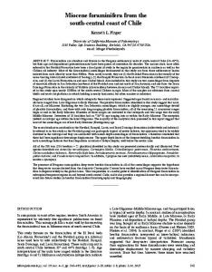
Fig. 2. Biological environmental data for comparison to foraminiferal distributions (see text for references). (A) Chlorophyll ‘a’ concentrations (mg chl a me3). The dashed line is the depth of the 1% light level. Note surface chl a maxima from 5”s to YN, particularly at 2”s and 2“N. The deep chlorophyll maxima at 7-9% from 75 to 100 m was associated with high concentrations of particles. (B) Primary productivity (mmol C m-3 day-‘) based on 14C uptake is highest at the surface in the equatorial region, particularly at 2”N and 2’3. The dashed line is the depth of the 1% light level. (C) >64-wm carbon concentrations (mm01 C mP3) from MOCNESS plankton tows, representing the biomass of macrozooplankton.

162


3.3. Biological environment The distribution and productivity of other plankton groups influence foraminiferal abundance. Most nonspinose foraminiferal species are herbivorous, while many spinose species consume macrozooplankton prey such as calanoid copepods (Spindler et al., 1984). The turbidity of productive waters lowers subsurface light levels, and could limit algal symbionts. These symbionts play a variable role in meeting the nutritional needs of several foraminiferal species (Hemleben et al., 1989). Surface chlorophyll concentrations surpassed 0.20 mg chl a rnw3 within the SEC from 5”S-3”N (Fig. 2a). Poleward of the SEC, surface chlorophyll concentrations decreased to less than 0.15 mg rnp3. The association of the SEC with higher chl a and nutrients suggests that advection from the east supplements local upwelling to support phytoplankton populations. Highest off the equator, surface chlorophyll reached >0.25 mg m-3 at 2”s and 2”N. The surface chlorophyll maxima at 2”N, with some patches measured at 5.0-29.0 mg chl rnp3, was associated with accumulation of the buoyant diatom Rhizosolenia at the convergent front on the edge of the tropical instability wave (Yoder et al., 1994). Strong upwelling at l“N, represented by shoaling isotherms, coincides with a strong subsurface chlorophyll maximum (>0.4 mg m-3) at 70 m. The equatorial minimum may be the result of strong surface divergences and upwelling of low biomass water, represented by low chlorophyll concentrations at 100-150 m from l”S-1”N. The weak subsurface chlorophyll maximum in this region may represent photoadaptation of phytoplankton with depth, rather than biomass maxima (Pak et al., 1988). Beam-c decreased with depth in the upper 80-100 m (Chung et al., 1996), while chl a concentrations increased, indicating an increase of chl acarbon ratios with depth. From 100 to 150 m, both beam-c and chl a linearly decreased. Primary productivity maxima at 2”s and 2”N (>2 mmol C rnp3 day-‘, Fig. 2b) correspond to biomass (surface chl a) maxima (Fig. 2a). Primary productivity integrated to the 0.1% light level depth peaked (>lOO mmol C me2 day-‘) from 3”S-2”N, with a slight equatorial minimum. South of 3”s and north of 2”N, integrated productivity dropped sharply to less

than 50 mmol C me2 day-’ (Barber et al., 1996). Across the transect, vertical maxima in primary productivity occurred within the saturating light levels of the upper 20 m (Fig. 2b). Low photosynthetic rates north of 5”N were associated with nitrate depletion in surface waters as well as low biomass. The carbon biomass of >64-pm zooplankton was highest (0.5-0.75 mm01 C mp3) from 2”S-2“N within the upper 60 m, and reached values of l-2 mmol C rnp3 in the presence of high phytoplankton standing stocks at the 2”N front (White et al., 1995Fig. 2~). Equatorial biomass was low (0.1 mm01 C rnp3) in the upper 20 m. A subsurface maximum (0.5 mmol C mp3) was present from 60-100 m from 3-5”s and 3-5”N. Biomass decreased to 0.1-0.2 mmol C me3 poleward of 5”N-5”s and below 100 m throughout the transect, consistent with primary productivity gradients. 3.4. Distribution offoraminifera Total standing stocks of living planktic foraminifera reached more than 100 shells mm3 within the upper 80 m from 3”S-3”N (Fig. 3). Standing stock maxima (>200 shells rne3) occurred off the equator, at the convergent front of 2”N from lo20 m and from 40-60 m at 3”s. Equatorial standing stocks were low, (50 shells rnT3. Foraminiferal abundance decreased north of 3% and below 100 m to less than 25 shells rne3.

1dos

5%

oo

5oN

latitude Fig. 3. Standing stocks of live planktic foraminifera (2150 pm shells mm3) recovered from 64-pm mesh MOCNESS plankton tows. Dots signify the midpoint of each sample interval, represented by the boxes on the right. The zero contour bounds samples with ~0.5 shells m-3.

163


G. menardii (shells

rnw3)

G. glum

(sheUs rnq3)

;;)JB,, lJ&.;A, lo?5

P. obliquiloculata(shellsmm31

10%

SOS

50s

o” latitude

5%

N. dutertrei (shells mv3)

00 latitude

Fig. 4. Standing stocks of foraminifera species common in the equatorial region (>150-pm glutinata, (C) I? obliquiloculata, (D) N. dutertrei.

Many species were most abundant within the upper 100 m in the equatorial region from S’S3”N. Globorotalia menardii (Fig. 4a) was present from S’S-S’N, but particularly abundant north of the equator. In the upper 60 m at 3“N, this species reached abundances of 15 shells rne3. Globigerinita glutinata was most abundant (20-30 shells me3) in the upper 60 m from 3”s to 3”N, excluding the equator (Fig. 4b). At 1“N this species was abundant to 100 m. Pulleniatina obliquiloculata (Fig. 4c) and Neogloboquadrina dutertrei (Fig. 4d) were abundant (lo-20 shells rnT3> from 1-3”s and l-3”N. The abundance of both species dropped sharply south of 5”s and north of 3”N. Globigerina bulloides, a species common in tropical upwelling systems but not present in the February-March samples (Watkins et al., 1996), was common within the upper 100 m from 3”s to 2”N (Fig. 5a). From 3”S-3”N, excluding 2“s and the equator, the standing stock averaged more than 10

shells m-‘). (A) G. menardii, (B) G.

shells mP3. The species reached its highest standing stock, 86 shells m-3, from lo-20 m at the convergence at 2”N. Other abundance maxima were from 40-60 m at 3”s and 1”N. Rare Globigerinella calida was most abundant (3 shells rne3) from l-3”N within the upper 60 m (Fig. 5b). The species Globigerinoides sacculifer, Globigerinoides ruber, and Globigerinoides conglobatus were abundant within the upper 80 m south of 5%. G. sacculifer had highest concentrations (more than 20 shells mP3) within the upper 60 m from 3-5”s (Fig. 6a). G. ruber had comparable maximum abundances within the upper 60 m from 1-3”s and l3”N (Fig. 6b). G. conglobatus was rare, most abundant south of 5-12”S, as well as from 2-3”N ~40 m (Fig. 6~). Maximum abundances of this species reached 5-8 shells mP3. Globoquadrina conglomerata (Fig. 7a) and Globorotalia tumida (Fig. 7b) were common south of the equator. Both species were abundant (lo-20

164


G. bull&es

+A

.

Micropaleontology

33 (1998) 157-I 74

(shells me31

. . .

. . .

G. sacarlifer (shells m-31

.

G. tuber (shellsm-3)

G.calida (shells mm31

,

.B

. . .

. . .

.

.

‘B ,’

200

10%

100s

50s

.I.

.“.

*

. L

I

5os

00

00

5%

latitude

latitude Fig. 5. Standing stocks of more foraminifera species common in the equatorial region (>lSO-pm shells m-3). (A) G. bulloides and (B) G. calida.

G. 0

conglobatus (shells rne3)

50

shells mP3) ~60 m at 1”s. The species also had prominent subsurface maxima south of this apparent outcrop area. Live G. tumidu were abundant (lo-15 shells me3) between 80 and 100 m from 2-5”s. The subsurface standing stock maximum of live G. conglomeratu (also lo-15 shells m-3) extended to 129 from loo-150 m, slightly deeper than G. tumidu. G. aequiluterulis was most abundant (lo-15 shells m-3) from 2-3”s from 40-100 m and at 1”N within the upper 100 m (Fig. 7~).

g s 8

‘O”

‘c)

150

??

.**

200

II 10%

. .

. . .

.

.

. . .

.

I+-?-+? 50s 6

* 9r.l

latitie Fig. 6. Standing stocks of foraminifera relatively important in the subtropical regions (>150+m shells mm3). (A) G. sacculifer, (B) G. ruber, (C) G. conglobatus.

3.5. Foraminiferal fauna1 assemblages

A Q-mode factor model grouped logarithmically transformed species percentages which covaried in the August plankton tows (Table 2). Loadings of three assemblages onto samples reveals simple spa-

tial patterns of relative abundance that account for 86% of the pooled variance (Table 3). An Equatorial Assemblage (Fig. 8a) composed of G. menardii, G. glutinata, P. obliquiloculata, N. dutertrei and G. bulloides was most prominent


G. conghnemta

Micropaleontology

(shells m-s

165

33 (1998) 157-174

Table 2 Factor scores from logarithmically abundance data from MOCNESS

transformed species percent tows of August-September,

1992 Species

G. menardii

100s

50s

G. glutinata P. obliquiloculata N. dutertrei G. bulloides G. calida

oo

latitude G. tumia’a (shellsrne3)

. . .

.

G.aepifaterufis (shellsrnq3) 0

.c 200

.

.I.

.

.

.

.

*

I ’ IT?+ 100s 5%

00

5%

latitude Fig. 7. Standing stocks of foraminifera common south of the equator (>150-pm shells mm3). (A) G. conglomerata, (B) G. tumida, (C) G. aequilateralis.

within the upper 200 m from l-3”N, within strong subsurface upwelling and near high accumulations of biomass at the strong convergent front on the edge of the tropical instability wave at 2”N. Its large scale distribution reflects the influence of the South

0.51 0.48 0.45 0.32 0.31 0.21

Subtropical

Southern deep

-0.21 0.08 -0.10 0.11 0.03 -0.12

0.00 0.03 0.17 0.09 -0.05 0.17

G. sacculifer G. ruber G. conglobatus

0.06 0.14 -0.03

0.66 0.56 0.34

0.00 -0.07 0.00

G. conglomerata G. tumida G. aequilateralis

0.06 -0.08 0.19

-0.20 0.01 0.05

0.78 0.46 0.33

Percentage of data explained

.f.

Equatorial

28

38

21

Total

86

Equatorial Current (SEC) and high phytoplankton biomass from 3”s to 3”N (Fig. la). The assemblage explained 38% of the species percent abundance variance. A Subtropical Assemblage composed of G. sacculifer, G. ruber, and G. conglobatus dominated the subtropical region south of Y’S and north of 5”N within the upper 100 m (Fig. 8b). This assemblage explained 28% of the variance. The assemblage was notably absent from S’S to 5”N at depths >80 m. The lowest surface water loadings for the Subtropical Assemblage were from l”S-3”N. The Deep Southern Assemblage (Fig. 8c; 21% of the variance) composed of G. conglomerata, G. tumida and G. aequilateralis was important >60 m from 2-12”s and at 5”N, outside of strongest subsurface upwelling indicated by shoaling isotherms (Fig. lc). The assemblage shoaled to the surface at 19, within high phytoplankton standing stocks, equatorial divergence and the SEC. 4. Discussion 4.1. The Equatorial Assemblage The Equatorial Assemblage (Fig. 8a) consisting of G. bulloides and herbivorous species G. menardii, G.

166


Micropaleontology

Table 3 Fauna1 factor loadings from logarithmically transformed species percent abundance dam from MOCNESS tows of AugustSeptember, 1992

33 (1998) 157-l 74

Table 3 (continued)

Latitude

Depth

Communality

Equatorial

Subtropical

Deep southern

Latitude

Depth

Communality

Equatorial

Subtropical

Deep southern

9 9 7 7 7 7 5 5 5 5 5 5 5 5 3 3 3 3 3 3 3 3 2 2 2 2 2 2

1 1 I I 1 1

I 1 0 0 0 -1 -1 -1 -1 -1 -1 -1 -2 -2 -2 -2

30 50 5 50 70 90 5 15 30 50 70 90 125 175 5 15 30 50 70 90 125 175 15 50 70 90 125 175 5 15 30 50 70 90 125 175 5 15 30 5 15 30 50 70 125 175 5 15 30 50

0.784 0.761 0.807 0.951 0.876 0.805 0.869 0.853 0.945 0.918 0.860 0.740 0.708 0.803 0.953 0.941 0.931 0.886 0.660 0.840 0.627 0.590 0.895 0.958 0.933 0.952 0.943 0.924 0.904 0.928 0.949 0.946 0.915 0.946 0.807 0.669 0.859 0.949 0.937 0.943 0.951 0.946 0.955 0.825 0.162 0.507 0.930 0.932 0.956 0.988

0.162 0.150 0.241 0.338 0.221 0.170 0.720 0.381 0.718 0.740 0.558 -0.142 -0.125 0.548 0.818 0.834 0.811 0.804 0.631 0.769 0.734 0.635 0.773 0.861 0.876 0.942 0.944 0.897 0.651 0.807 0.822 0.832 0.809 0.878 0.886 0.773 0.703 0.844 0.793 0.641 0.624 0.625 0.611 0.572 0.185 0.547 0.623 0.594 0.503 0.717

0.864 0.829 0.854 0.912 0.900 0.773 0.560 0.712 0.629 0.545 0.203 0.145 0.159 0.065 0.493 0.465 0.484 0.409 0.247 0.293 0.071 -0.084 0.515 0.437 0.360 0.180 0.197 0.309 0.676 0.485 0.493 0.477 0.473 0.354 -0.085 0.266 0.463 0.467 0.413 0.503 0.502 0.556 0.521 0.340 0.044 -0.118 0.608 0.634 0.610 0.480

0.108 0.227 0.139 0.077 0.131 0.422 0.195 0.448 0.182 0.270 0.713 0.836 0.817 0.707 0.202 0.172 0.198 0.269 0.448 0.403 0.289 0.424 0.178 0.163 0.188 0.177 0.119 0.151 0.152 0.203 0.174 0.160 0.195 0.222 0.121 0.03 1 0.388 0.138 0.369 0.528 0.556 0.496 0.556 0.618 0.355 0.441 0.417 0.42 1 0.575 0.494

-2 -2 -2 -2 -3 -3 -3 -3 -3 -3 -3 -3 -5 -5 -5 -5 -5 -5 -5 -5 -12 -12 -12 -12 -12

70 90 125 175 5 15 30 50 70 90 125 175 5 15 30 50 70 90 125 175 5 70 90 125 175

0.966 0.972 0.915 0.739 0.929 0.905 0.942 0.894 0.864 0.934 0.969 0.632 0.942 0.958 0.952 0.950 0.905 0.880 0.942 0.853 0.900 0.864 0.856 0.699 0.860

0.600 0.569 0.644 0.396 0.629 0.607 0.622 0.597 0.632 0.415 0.569 0.667 0.561 0.495 0.487 0.498 0.378 0.276 0.070 0.330 0.242 0.266 0.194 0.054 0.106

0.494 0.398 0.326 0.432 0.602 0.595 0.589 0.591 0.506 0.372 0.149 -0.230 0.695 0.705 0.742 0.662 0.587 0.353 0.202 0.205 0.910 0.890 0.822 0.595 0.637

0.602 0.700 0.627 0.629 0.414 0.426 0.456 0.433 0.457 0.790 0.790 0.367 0.379 0.464 0.406 0.513 0.645 0.824 0.947 0.838 0.120 -0.027 0.377 0.584 0.666

glutinata, R obliquiloculata, N. dutertrei confirms previous observations of these species in cool and productive tropical upwelling settings. G. menardii and R obliquiloculata are equatorial species, with G. menardii most abundant to the east and P. obliquiZoculata more common in the central equatorial Pacific (Bradshaw, 1959). Wider ranging N. dutertrei thrives in temperate and tropical coastal upwelling settings, as well as living in equatorial open-ocean environments (Bradshaw, 1959; Fairbanks et al., 1982). G. buZZoides, although common in subpolar regions, seasonally dominates cool surface waters of tropical coastal upwelling in the eastern equatorial Pacific (Thiede, 1983), the Arabian Sea (Prell and Curry, 1981; Auras-Schudnagies et al., 1989), Venezuela (Cifelli and Smith, 1974) and Northwest Africa (Oberhansli et al., 1992). G. ghtinata occurred at high frequencies just outside of coastal upwelling off Peru (Thiede, 1983). These species are associated with abundant phytoplankton and high productivity. N. dutertrei standing


Micropaleontology

Equatorial faunal factor

100s

5%

00

50s

latitude Subtropical faunaI factor

00 50N latitude Deep Southern faunal factor

100s

50s

.

loos

50s

. . . . . .

. . . . .

. .

.

.

oo

latitude Fig. 8. Factor loadings of Q-mode fauna1 factors, based on logarithmically transformed species percent abundance data. See Table 2 for factor scores. Note that patterns of factor loadings represent simplifications of the relative abundance patterns of the species, rather than standing stocks. (A) The Equatorial Assemblage, dominated by nonspinose herbivorous species G. menardii, G. glutinata, t! obliquiloculata, N. dutertrei and spinose herbivores G. bulloides and G. calida. (B) The Subtropical Assemblage, containing spinose, dinoflagellate symbiont bearing species G. sacculifer, G. ruber, and G. conglobatus. (C) The Deep Southern Assemblage, containing nonspinose species G. conglomerata and G. tumida, and spinose G. aequilateralis.

33 (1998) 147-174

167

stocks (O-100 m average) are very low at low productivity levels (~60 mm01 C rnA2 day-‘), but level off near 7 shells me3 at higher productivity levels (Fig. 9a). Standing stocks (O-100 m average) of P. obliquiloculata (r 2 = 0.83) increase linearly with integrated primary productivity (Fig. 9a). Standing stocks of G. bulloides and G. menardii also increase at high productivity levels, but suggest a threshold near 90 mmol C rnw2 day-‘, above which both species standing stocks increase exponentially (Fig. 9b). The relative abundance of G. bulloides also increases exponentially above this level of productivity (Fig. SC). These relationships are consistent with their association with high productivity environments. Standing stocks of these species were low directly on the equator (Fig. 3), consistent with patterns of phytoplankton and macrozooplankton biomass (Fig. 2a,c). This pattern reflects water being upwelled from depths >80 m (Murray et al., 1994) with low plankton biomass. Strong divergence (2060 cm SK’) could advect continually upwelled water 1” off the equator in less than a week, so that high standing stocks of foraminifera 1” north and south of the equator (four fold increase) reflect a rapid response by foraminifera. Standing stocks were also high at convergent fronts near 2”N and 3’S, where water downwells and recirculates back to the equator. High standing stocks of the buoyant diatom species RhizosoEenia were observed at the front at 2”N associated with the tropical instability wave (Yoder et al., 1994). The rapid growth of foraminifera and their similar use of buoyancy in regions of convergence may be responsible for the strong correlation of herbivorous species standing stocks and integrated primary productivity in August. High standing stocks of the Equatorial Assemblage from 3”S-3”N were also associated with the zonal advection by the South Equatorial Current (SEC) (Fig. 8a and Fig. la). As observed in February, the strong SEC (up to 60 cm SK’) may advect foraminiferal fauna from equatorial upwelling regions east of the transect (Watkins et al., 1996). In August, highest standing stocks of foraminifera were within the current. Therefore, advection by the SEC is a potentially important source and sink for local foraminiferal populations at 14O”W. The productive local conditions could support these

168


species, thus they are unlikely to be ‘terminal immigrants’ (Bradshaw, 1959). Therefore, we consider the foraminiferal fauna a good proxy of local conditions. Equatorial Assemblage species were abundant throughout the upper 60-100 m, and did not have a consistent subsurface maximum. Standing stocks dropped sharply below these depths near the base 15 ??N. dutertrei

0 P. obliquilomlata --

of the euphotic zone (60-80 m) and the thermocline (120 m). Phytoplankton prey and facultative algal symbionts (Gastrich, 1987) depend on light and therefore may influence the distribution of these species below the euphotic zone. Water temperatures from 100-200 m ranged from 12-20°C. iV dutertrei and G. bulloides, common in temperate-subpolar regions, are thought to bloom when upwelling shoals their cool habitat within the productive photic zone (Curry et al., 1983; Reynolds Sautter and Thunell, 199 1; and Ravelo and Fairbanks, 1992). In this study, the two species lived within 22-25°C water of the upper 80 m, consistent with previous observations in tropical upwelling regions (Prell and Curry, 1981 and Oberhansli et al., 1992). 4.2. The Subtropical Assemblage and oligotrophic regions

20

40

60 80 100 120 integrated primary productivity

140

(mmol C me2 d-l)

o 3”N

d B 20

40

60 80 100 integrated primary productivity

120

. 140

(mmol C me2 d-l) 251

.

,

.

,

.

,

.

,

*

,,.

,

0

20

40

integ%d p&y

prod&&y

(mmol C me2 d-l)

120

Outside the 5”N-5’S equatorial zone, foraminifera were dominated by the Subtropical Assemblage composed of G. sacculifer, G. ruber, and G. conglobatus (Fig. 8b). These species have adapted to oligatrophic conditions by exploiting dinoflagellate endosymbionts, which contribute substantially to the growth of their hosts (Caron et al., 1981; Gastrich and Bartha, 1988). In this study, these species tolerated low integrated primary productivity levels (2040 mm01 C m-’ day-‘) and low concentrations of surface chlorophyll (to.15 mg rnm3) and >64+m zooplankton biomass (co.2 mmol C m-3).

140

Fig. 9. Relationship of herbivorous species standing stock to integrated primary productivity (mmol C m-* day-‘). (A) N. dutertrei (filled circles) is most abundant (7 shells m-s) at productivities 260 mmol C m-’ day-‘. f! obliquiloculatu (open circles, y = -1.66 + 0.09x, r* = 0.83) is linearly related to productivity. Standing stock is averaged from 0 to 100 m. (B) Standing stock (shells mp3) of G. bulloides (filled circles, y = 0.0027e0.070X, r2 = 0.69) and G. menarrfii (open circles, y = 0.054e0.057X, r2 = 0.83) exponentially increase at productivity levels >90 mmol C m-* day-‘. Note one observation of high standing stock for G. menardii at 3”N, just north of TIW front, which is not included in regression equation. Standing stock is averaged from 0 to 100 m. (C) Percent abundance of G. bulloides. Percent abundance is percentage of total foraminifera from 0 to 100 m. The percent abundance of this species exponentially increases at productivity levels >90 mmol C m-2 day-t (y = 0.0048e0-M9X, r2 = 0.80).

169


Neither the cooler temperatures or lower subsurface light levels within the equatorial ‘cold tongue’ influenced standing stocks of Subtropical Assemblage species. Within the upper 60 m, these species were as abundant in equatorial waters as within the subtropical region south of S’S (Fig. 6). Their success within 22-28°C water is consistent with the thermal tolerance ranges of G. sacculifer (14-32”C), G. ruber (14-32°C) and G. conglobatus (13-30°C) from controlled culture experiments (Bijma et al., 1990a). In general, the vertical distribution of these species was also consistent with subsurface light levels. Assuming a compensation light level for G. sacculifer of 26-30 PEin m-* s-’ (Jorgensen et al., 1985) and an average surface irradiance of 35 Ein m-* day-’ (Newton and Murray, JGOFS data system), this species needed to live above the 6.5% light level to balance its respiration needs for one day. For most of the transect, this light level corresponds to a depth of 45-50 m and is consistent with the sharp decrease in the abundance of G. sacculifer below 60 m (Fig. 6a). However, the vertical distribution of this species at l-2”N or 3’S, where this compensation light level shoals near 35 m, does not differ from its vertical distribution at 12‘S, where the compensation light level is near 70 m. The percent abundance of G. sacculifer is high (20-50% of total foraminifera) at low productivity levels t40 mmol C mP2 day-’ (r = 0.51, Fig. 10). The dominance of this species off the equator is produced by the rarity of herbivorous species within low-productivity waters (Fig. 9). G. sacculifer maintains a relative abundance near 10% of total foraminifera at productivity levels >40 mm01 C m-* day-’ (Fig. 10). 4.3. The Deep Southern Assemblage The Deep Southern Assemblage, composed of G. conglomerata, G. tumidu, and G. aequilateralis dominated from 80-200 m in the Southern Hemisphere (Fig. 8~). The deep standing stock maxima (So-150 m) of G. conglomerata and G. tumida are the most prominent feature of this assemblage, which otherwise dominates deep samples with very low total standing stocks. These species were abundant near the base of the euphotic zone, and well below abundance maxima of phytoplankton and zooplankton.

0

I

20

40

e

I

60

I

I

80

r

I

,

100

1

120

I

140

integrated primary productivity (mmol C mm2d-1) Fig. 10. Relationship of the percent abundance of G. sacculifer with integrated primary productivity (mm01 C mm2 day-‘). Percent abundance of G. sacculifer is highest at productivity levels less than 40 mm01 C mm2 day-‘, above which the species comprises 10% of foraminifera (y = 33.3e-“~o’oX, r2 = 0.49). An exception is the high percentage of G. sacculifer within productivity levels of 70 mm01 C mm2 day-’ at 5”s. Percent abundance is percentage of total foraminifera from 0 to 100 m.

They lived above the deep thermocline, within water temperatures ranging from 22-26°C. From l-3?& low standing stocks below 100 m were associated with a shallow (125 m) thermocline. Standing stocks of G. conglomerata and G. tumidu shoaled at l”S, and indicate that the species also live in the upper ocean. The strong surface divergence south of the equator is consistent with the upwelling of the deep fauna (Fig. lb). However, temperature (Fig. lc) and nutrient profiles at 1”s do not confirm upwelling. Primary productivity and chl a concentration are high here (Fig. 2). Surface waters north and south of 1”s also had high phytoplankton activity, and low standing stocks of these species. At 5“N, G. conglomeratu was evident from lo-150 m, but at much lower standing stocks than south of the equator (Fig. 7a). From l-2”N, the rarity of this species is associated with strong upwelling, where isotherms strongly shoaled. 4.4. Comparison to El NiAo fauna: G. bulloides The appearance of G. bulloides in ‘cold tongue’ conditions signifies a major fauna1 shift. In interpreting the appearance of this species, common in tropical coastal upwelling settings, we need to separate

170


Micropaleontology

contributions of food abundance, SEC advection, and water temperature. G. bulloides feeds on phytoplankton, zooplankton, and small naupliar larvae (H. Spero, personal communication). The abundance of plankton food, rather than temperature, was associated with the abundance of this omnivorous species within the temperate California Current coastal upwelling system (Ortiz et al., 1995). High standing stocks of the species occurred only within turbid coastal waters with high >64 ,um plankton displacement volumes (Pdv) from 5-9 ml rnp3. This apparent food threshold is consistent with our >64+m Pdv measurements of 5 ml rnp3 (0.550.75 mm01 C me3 in carbon biomass measurements) associated with high standing stocks of G. bulloides from I-2”N. The species was absent during El NiAo, when Pdv was t3 ml m-3. A food threshold for G. bulloides is also apparent in the relationship of its abundance with primary productivity in August. The standing stock and percent abundance of G. buZZoides were low within waters of productivity levels t90 mm01 C me2 day-‘, above which both exponentially increase (Fig. 9). Integrated primary productivity nearly doubled from February to August to >lOO mm01 C m-* day-’ from 3”S-2”N (Murray et al., 1994). Therefore, the appearance of G. bulloides in August is consistent with a significant increase in food resources represented by autotrophic and heterotrophic standing stocks. G. buZZoides not only tracked the increase in equatorial food abundance and primary productivity in August, but also paralleled community shifts which may be responsible for this change. Diatoms, including many large species common to coastal upwelling regions, increased from to. 1% of total chlorophyll in February to 6% in August (Murray et al., 1994). Diatom abundance has been previously correlated (I = 0.78) to integrated primary production in this region (Chavez et al., 1990). Iron supply from the shoaled EUC may have stimulated the growth of large phytoplankton in August (Murray et al., 1994). However, an alternative explanation for the success of these phytoplankton is the higher survival of seed populations within the SEC. The appearance of foraminifera common in coastal upwelling ecosystems (e.g. G. bulloides) is consistent with an advective influence. Aided by SEC advection, immature upwelling communities expanded westward during

33 (1998) 157-174

the intensification of upwelling. We infer that G. bulloides tracks this process in the central equatorial Pacific, and thus may be a good geologic proxy for high biomass waters. In contrast to patterns observed during La Nina cool conditions, phytoplankton and foraminiferal abundance were relatively low within the SEC core at 2”s during El Nifio (Watkins et al., 1996). Both were most abundant north of the equator within a convergence at the SECYNECC boundary. Flowing at a consistent velocity, the SEC appears to contain more phytoplankton and foraminifera during ‘cold tongue’ conditions than during the El Niiio. This increase in particle load is consistent with stronger upwelling and higher productivity east of the 14O”W transect in August. The La Nina SEC could be more successful in seeding local populations within favorable high-food conditions along its transit across the Pacific than within the food-poor El Nifio setting. 4.5. Comparison

to El Niiio fauna: South Equatorial and Equatorial Assemblages

The Equatorial Assemblage of August (this paper) and the North Equatorial Assemblage of February (Watkins et al., 1996) were both important north of the equator. However, the presence of G. menardii and G. glutinata and the absence of G. conglomerata and G. tumida suggests a closer association of the August Equatorial Assemblage with the South Equatorial Assemblage of February. Species of February’s South Equatorial Assemblage, associated with the SEC, had low standing stocks. We have interpreted the assemblage as a population advected into unfavorable conditions (Watkins et al., 1996). Also generally associated with the SEC, August’s Equatorial Assemblage represented the transect’s highest foraminiferal standing stocks. This reflects the intensification of upwelling and higher primary productivity in August. Local productive conditions in August were considerably more favorable to assemblage species seeded by SEC advection, including upwelling indicators G. menardii and G. bulZoides. Higher standing stocks of the two species, although often off the equator at convergent fronts, were consistent with the westward expansion of upwelling communities. I? obliquiloculata, N. dutertrei, and G. glutinata had high standing stocks from 3”S-


3”N in August, rather than only within a northem convergent setting as in February. Their higher standing stocks south of the equator, within the SEC, suggest higher primary productivity and plankton populations east of the 14O”Wtransect. 4.6. Comparison Assemblages

to

El NiAo fauna: Subtropical

In both February (Watkins et al., 1996) and August (this paper), a Subtropical Assemblage composed of G. sacculifer, G. ruber, and G. conglobatus dominated oligotrophic regions outside the 5”S-5”N equatorial zone. Up to 30-50% of total foraminifera in these settings were G. sacculifer. Their persistent dominance of subtropical regions reflects unchanged conditions. Surface chlorophyll concentrations (0.10-0.15 mg chl me3), integrated primary productivity (~50 mm01 C rnp2 day-‘) and surface nutrients (undetectable) were consistently low in February and August. Low zonal velocities and isolation from equatorial meridional circulation may impede the importation of fauna from other regions. G. sacculifer maintained consistent populations of lo-20 shells mm3 for February and August. From February to August, the 24°C isotherm shoaled from 125 m to 50 m and the 1% light level shoaled from 85 m to 60 m near the productive convergent front (l-2“N). However, these light levels and temperatures do not limit the species in controlled culture experiments (Jorgensen et al., 1985 and Bijma et al., 1990a), and are consistent with stable standing stocks. The species also maintained a relative abundance near 10% of total foraminifera in this productive region. Although associated with subtropical environments, the abundance of G. ruber from 3”S-3”N in the upper 60 m increased from 20 shells rnp3 in August. Standing stock of this species increased with integrated primary productivity (r2 = 0.56) in August. G. ruber has been previously associated with higher productivity regions. For example, G. ruber replaces G. sacculifer as the dominant species in the plankton and sediments of the southern Red Sea as productivity increases toward the Arabian Sea. This shift has been attributed to G. ruber’s greater dependence on phytoplankton food (Auras-Schudnagies et al.,

171

1989) or symbiont photosynthesis (limited by nutrients, Bijma et al., 1990b) relative to G. sacculifer’s primarily zooplankton diet. A shorter life cycle (14 relative to 28 days as inferred by Bijma et al., 1990b) may permit G. ruber to thrive in the highly variable environment of fertile regions as an opportunistic species. However, the role of this species in the Subtropical Assemblage still emphasizes this species has high relative abundances within low productivity regions. 4.7. Comparison to El NiAo fauna: North Equatorial and Deep Southern Assemblages In both February (Watkins et al., 1996) and August (this paper), G. conglomerata and G. tumida were associated with each other. These species, particularly G. conglomerata, had deep abundance maxima from 80-150 m, near the base of the euphotic zone. However, their abundance maxima rarely extended below the deep thermocline, and suggested temperature limitation below 20°C. From February to August, their standing stocks dramatically decreased within the O-5”N region as mixed layer depth shoaled from 100 to 50 m. Their association with deep mixed layers is consistent with their affinity to western equatorial Pacific settings (Bradshaw, 1959). These species were also abundant in the upper surface ocean, usually associated with high chl a concentrations. However, they were much more common in surface waters during February. In February, the two species, joined by I? obliquiloculata and N. dutertrei, represented the highest foraminiferal standing stocks in the region, within a local convergence from l-3”N with high concentrations of phytoplankton biomass. In August, they were abundant at the surface only at 1”s. 4.8. Comparison to El Nifio fauna: role of meridional circulation During El Nifio conditions, meridional velocities near the equator were relatively weak (10 km day-‘). Foraminifera within equatorial waters could have been advected for a month, a timescale close to their lifespan (Hemleben et al., 1989), before the water recirculates at convergences 3” north and south of the

172


equator. Different fauna north and south of the equator suggests that meridional advection of equatorial fauna was not important in February (Watkins et al., 1996). Slow meridional circulation provides time for fauna advected north and south of the equator to diverge through the influence of other processes. Fauna north of the equator were influenced by a population within a region of convergence observed at 3”N, 14O“W, while fauna south of the equator, within the SEC, may have had time to be advected from regions of upwelling far to the east. Within La Nina conditions, meridional velocities were very strong (up to 50 km day-‘) due to the passage of the tropical instability wave. A single equatorial fauna spread from 3“N-3’S (Fig. 8) suggests that the dynamic meridional circulation thoroughly mixed foraminifera in this region. Surface water of this region may have upwelled on the equator as recently as a week before sampling, little time to alter foraminiferal fauna. Water recirculates at convergent fronts near 2”N and 3’S, resulting in a barrier to the dispersal of equatorial fauna out of this region. High concentrations of foraminifera at convergent fronts suggests that foraminifera use buoyancy to maintain their position within these food-rich zones. During February, foraminifera were most abundant (130 shells m-3) within a weak convergence at 3”N near the SEUNECC boundary. In August, high standing stocks (250 shells rne3) occurred at the strong convergent front of 2”N associated with the tropical instability wave. Strong convergences north of the equator have been attributed to the shear of the SEC with the NECC. In August, high standing stocks of foraminifera and diatoms at 1-3‘S suggest that buoyancy is also used within convergent fronts south of the equator, near the boundary of the SEC with subtropical waters to the south. High standing stocks are the result of favorable conditions over the previous reproductive cycle which promote reproductive success for the previous generation, as well as juvenile survivorship (Spero, personal communication). Therefore, high stocks reflect the availability of diverse food supplies during the previous month to both juveniles and adults. This includes not only the supply of large phytoplankton such as diatoms to adults, but also an ample supply of picophytoplankton for juveniles. More than 95% of the primary productivity in this region is by cells

~2 ,um in size (Murray et al., 1994), further emphasizing that the correlation of standing stocks and primary productivity may largely be a reflection of juvenile food supplies. The convergence zones have a large and diverse array of food for several life stages, suggesting that the population may maintain their position within these features through much of their life cycle. 4.9. Foraminifera as paleoceanographic proxies The fauna1 assemblages we have identified in living planktic foraminiferal populations of February and August at 14O”W in the equatorial Pacific strongly correspond to three core-top sediment assemblages in the tropical Atlantic Ocean (Ravelo et al., 1990). These sediment faunal assemblages were weakly correlated to modem sea-surface temperatures (ranging from 17-30°C) in the tropical Atlantic Ocean. They were more strongly associated with changes in mixed layer depth (using definition of Levitus, 1982). Our Subtropical Assemblage, dominated by G. ruber and G. sacculifer, corresponds to the Mixed Layer Factor of Ravelo et al. (1990) in the Atlantic Ocean sediments, associated with deep (>35 m) mixed layers. Mixed Layer Factor loadings were exponentially related to mixed layer depth, and highest within deep mixed layers. N. dutertrei, G. tumida, I? obliquiloculata and G. menardii, important components of our equatorial fauna, dominate the Tropical Atlantic Thermocline Factor of Ravelo et al. (1990). G. bulloides, observed only in our equatorial fauna during August, is an important component of the Tropical Atlantic Seasonal Succession Factor by Ravelo et al. (1990). The sum of the Thermocline and Seasonal Succession Factor loadings were inversely correlated with mixed layer depth, and suggested that these species prefer shallow (~35 m) mixed layers. The observations of Ravelo et al. (1990) suggest that Subtropical Assemblage species would dominate surface waters above the deep (60-100 m) thermocline of our central Pacific transect. Our observation of diverse fauna in the JGOFS transect suggests that other parameters, including primary productivity, can play a more important role here than thermocline depth. Ravelo et al. (1990) did not


Micropaleontology

evaluate the influence of primary productivity, although integrated primary productivity and nitricline depth in the tropical Atlantic are inversely correlated (r2 = 0.84, Herbland and Voituriez, 1979). This inverse relationship holds best for stratified settings with depleted surface nutrients. However, our transect includes equatorial stations with a deep thermocline but high productivity stimulated by the upwelling of nutrients. This upwelling influence results in a weak overall correlation of primary productivity and mixed layer depth within our data set (r* = -0.03). We observed a range of primary productivity comparable to that of the entire tropical Pacific in a transect with a deep thermocline. The faunal changes we observed are more closely associated with primary productivity levels than with mixed layer depth. 5. Conclusions The occurrence of G. bulloides, a species commonly also found in tropical coastal upwelling, in equatorial surface waters in August was consistent with higher primary productivity and advection within the SEC ‘cold tongue’. The standing stock and relative abundance of this species exponentially increased within integrated primary productivity levels above 90 mmol C m-2 day-‘. The species also accompanied an increase in the role of large diatoms. Both associations reflect a high biomass system. The SEC may have seeded these coastal species from the east as their productive upwelling habitat expanded westward. One equatorial fauna1 assemblage dominated the high surface standing stocks of foraminifera from 3”S-3”N, consistent with seeding by the SEC and vigorous meridional circulation. Convergent fronts 2-3” north and south of the equator, where water advected from the equator recirculates, represent physical barriers to the dispersal of equatorial fauna. High standing stocks of foraminifera within these productive fronts reflects their use of buoyancy to take advantage of high food stocks. The ecology of species in the two surface assemblages is consistent with the shift along the transect from oligotrophic subtropical settings, dominated by symbiont bearing species, to productive upwelling settings, dominated by herbivorous species. The

33 (1998) 157-174

113

herbivorous species of the Equatorial Assemblage were rare within subtropical surface waters, apparently limited by low phytoplankton abundance. High standing stocks of symbiont bearing species within the productive equatorial region indicate that these species benefit from high food abundance. Acknowledgements We would like to thank US JGOFS collaborators L. Welling, J. White and M. Roman (who collected the plankton tows), R. Barber (responsible for primary productivity) and J. Murray (hydrography) as well as others who assisted at sea and in the laboratory. A. Morey provided taxonomic assistance. H. Spero and an anonymous reviewer helped to improve the manuscript. This project was funded under NSF Grant OCE-90-22299. This paper is US JGOFS contribution number 437. References Auras-Schudnagies, A., Kroon, D., Ganssen, G., Hemleben, Ch., Van Hinte, J.E., 1989. Distributional pattern of planktonic foraminifers and pteropods in surface waters and top core sediments of the Red Sea and adjacent areas controlled by the monsoonal regime and other ecological factors. Deep-Sea Res. 36, 1515-1533. Barber, R.T., Sanderson, M.P., Lindley, S.T., Chai, F., Newton, J., Trees, C., Foley, D.G., Chavez, El!!, 1996. Primary productivity and its regulation in the equatorial Pacific during and following the 1991-1992 El Nifio. Deep-Sea Res. I1 43, 933-970. Bidigare, R.R., Ondrusek, M.E., 1996. Spatial and temporal variability of phytoplankton pigment distributions in the central equatorial Pacific Ocean. Deep-Sea Res. II 43, 809-833. Bijma, J., Faber, W.W.Jr., Hemleben, Ch., 1990a. Temperature and salinity limits for growth and survival of some planktonic foraminifers in laboratory cultures. J. Foraminiferal Res. 20, 95-l 16. Bijma, J., Erez, J., Hemleben, Ch., 1990b. Lunar and semi-lunar reproductive cycles in some spinose planktonic foraminifers. J. Foraminiferal Res. 20, 117-127. Bradshaw, J.S., 1959. Ecology of living planktonic foraminifera in the North and Equatorial Pacific Ocean. Cushman Found. Foraminiferal Res. Co&b. 10, 25-64. Caron, D.A., Be, A.W.H., Anderson, O.R., 1981. Effects of variations in light intensity on life processes of the plauktonic foraminifera Globigerinoides sacculifer in laboratory culture. J. Mar. Biol. Assoc. U.K. 62.435-452. Chavez, EP, Buck, K.R., Barber, R.T., 1990. Phytoplankton taxa in relation to primary production in the equatorial Pacific. Deep-Sea Res. 37, 1733-1752.

174


Micropaleontology

Chung, S.P., Gardner, W.D., Richardson, M.J., Walsh, I.D., Landry, M.R., 1996. Beam attenuation and micro-organisms: spatial and temporal variations in small particles along 14O”W during the 1992 JGOFS EqPac transects. Deep-Sea Res. II 43, 1205-1226. Cifelli, R., Smith, R.K., 1974. Distributional patterns of planktonic foraminifera in the western North Atlantic. J. Foraminiferal Res. 4, 112- 125. Curry, W.B., Thunell, R.C., Honjo, S., 1983. Seasonal changes in the isotopic composition of planktonic foraminifera collected in Panama Basin sediment traps. Earth Planet. Sci. Lett. 64, 33-43. Fairbanks, R.G., Sverdlove, MS., Free, R., Wiebe, PH., Be, A.W.H., 1982. Vertical distribution and isotopic fractionation of living planktonic foraminifera from the Panama Basin. Nature 298, 841-844. Gardner, W.D., Chung, S.P., Richardson, M.J., Walsh, I.D., 1995. The oceanic mixed-layer pump. Deep-Sea Res. II 42, 757776. Gastrich, M.D., 1987. Ultrastmcture of a new intracellular symbiotic alga found within planktonic foraminifera. J. Phycol. 23,623-642. Gastrich, M.D., Bartha, R., 1988. Primary productivity in the planktonic foraminifer Globigerinoides ruber (D’Orbigny). J. Foraminiferal Res., 18, 137-142. Hemleben, Ch., Spindler, M., Anderson, O.R., 1989. Modem Planktonic Foraminifera. Springer-Verlag, Berlin. Herbland, A., Voituriez, B., 1979. Hydrological structure analysis for estimating primary production of the tropical Atlantic Ocean. J. Mar. Res. 37, 87-101. Johnson, E.S., 1996. A convergent instability wave front in the central tropical Pacific. Deep-Sea Res. II 43,753-778. Jorgensen, B.B., Erez, J., Revsbech, N.P., Cohen, Y., 1985. Symbiotic photosynthesis in a planktonic foraminiferan, Globigerinoides sacculifer (Brady), studied with microelectrodes. Limnol. Oceanogr. 30, 1253-1267. Levitus, S., 1982. Climatological Atlas of the World Ocean. NOAA Professional Paper 13. Michaels, A.F., Silver, M.W., 1988. Primary production, sinking fluxes and the microbial food web. Deep-Sea Res. 35, 473490. Murray, J.W., Barber, R.T., Roman, M.R., Bacon, M.P., Feely, R.A., 1994. Physical and biological controls on carbon cycling in the Equatorial Pacific. Science 266, 58-65. Murray, J.W., Johnson, E., Garside, C., 1995. A US JGOFS process study in the Equatorial Pacific (Eq Pat): Introduction.

33 (I 998) 157-l 74

Deep-Sea Res. I1 42, 275-294. Oberhlnsli, H., Benier, C., Meinecke, G., Schmidt, H., Schneider, R., Wefer, G., 1992. Planktonic foraminifers as tracers of ocean currents in the eastern South Atlantic. Paleoceanography 7,607-632. Ortiz, J.D., Mix, A.C., Collier, R.W., 1995. Environmental control of living symbiotic and asymbiotic foraminifera of the California Current. Paleoceanography 10,987-1010. Pak, H., Kiefer, D.A., Kitchen, J.C., 1988. Meridional variations in the concentration of chlorophyll and microparticles in the North Pacific Ocean. Deep-Sea Res. 35, 1151-1171. Prell, W.L., Curry, W.B., 1981. Fauna1 and isotopic indices of monsoonal upwelling: Western Arabian Sea. Oceanol. Acta 4, 91-98. Ravelo, A.C., Fairbanks, R.G., 1992. Oxygen isotopic composition of multiple species of planktonic foraminifera: recorders of the modem photic zone temperature gradient. Paleoceanography 7, 815-83 1. Ravelo, A.C., Fairbanks, R.G., Philander, S.G.H., 1990. Reconstructing tropical Atlantic hydrography using planktonic foraminifera and an ocean model. Paleoceanography 5, 409431. Reynolds Sautter, L., Thunell, R.C., 1991. Seasonal variability in the ‘*O and t3C of planktonic foraminifera from an upwelling environment: sediment trap results from the San Pedro Basin, Southern California. Paleoceanography 6, 307-334. Spindler, M., Hemleben, Ch., Salomons, J.B., Smit, L.P, 1984. Feeding behavior of some planktonic foraminifers in laboratory cultures. J. Foraminiferal Res. 14, 237-249. Thiede, J., 1983. Skeletal plankton and nekton in upwelling water masses off northwestern South America and Northwest Africa. In: Suess, E., Thiede, J. (I%.), Coastal Upwelling: Its Sediment Record, Part A: Responses of the Sedimentary Regime to Present Coastal Upwelling. Plenum Press, New York. Watkins, J.M., Mix, A.C., Wilson, J., 1996. Living planktic foraminifera of the central Equatorial Pacific Ocean: tracers of circulation and productivity regimes. Deep-Sea Res. II 43, 1257-1282. White, J.R., Zhang, X., Welling, L., Roman, M.R., Dam, H.G., 1995. Latitudinal gradients of zooplankton biomass in the tropical Pacific at 14O”W along the JGOFS Eq Pat study: Effects of El Nitio. Deep-Sea Res. II 42.715-734. Yoder, J.A., Ackleson, S.G., Barber, R.T., Flament, I?, Balch, W.M., 1994. A line in the sea. Nature 371,689-692.