5500
IEEE TRANSACTIONS ON SIGNAL PROCESSING, VOL. 56, NO. 11, NOVEMBER 2008
Localization of Narrowband Radio Emitters Based on Doppler Frequency Shifts Alon Amar, Student Member, IEEE, and Anthony J. Weiss, Fellow, IEEE
Abstract—Several techniques for emitter localization based on the Doppler effect have been described in the literature. One example is the differential Doppler (DD) method in which the signal of a stationary emitter is intercepted by at least two moving receivers. The frequency difference between the receivers is measured at several locations along their trajectories and the emitter’s position is then estimated based on these measurements. This twostep approach is suboptimal since each frequency difference measurement is performed independently, although all measurements correspond to a common emitter position. Instead, a single-step approach based on the maximum likelihood criterion is proposed here for both known and unknown waveforms. The position is determined directly from all the observations by a search in the position space. The method can only be used for narrowband signals, that is, under the assumption that the signal bandwidth must be small compared to the inverse of the propagation time between the receivers. Simulations show that the proposed method outperforms the DD method for weak signals while both methods converge to the Cramér–Rao bound for strong known signals. Finally, it is shown that in some cases of interest the proposed method inherently selects reliable observations while ignoring unreliable data. Index Terms—Differential Doppler (DD), emitter location, maximum-likelihood estimation.
I. INTRODUCTION
P
ASSIVE position determination of a radiating emitter has been discussed in the literature since World War II. The position can be estimated by measuring one or more location-dependent signal parameters such as angle of arrival, time of arrival, received signal strength or Doppler frequency shift [1]–[4]. The idea of using the Doppler effect for localization found applications in radar, sonar, passive location systems (both for radio signals and acoustic signals), satellite positioning and navigation. To simplify the exhibition of our ideas we have chosen to address a specific application of localization using the Doppler effect. We focus on locating a stationary radio emitter by moving receivers. The motion induces frequency shift that is proportional to the signal frequency and to the radial velocity of each receiver towards (or away from) the emitter. It is assumed that the receiver location and velocity are known and therefore the emitter location can be estimated. Manuscript received August 17, 2007; revised April 8, 2008. First published August 19, 2008; current version published October 15, 2008. The associate editor coordinating the review of this paper and approving it for publication was Dr. Mats Bengtsson. This research was supported by the Israel Science Foundation (Grant 1232/04). The authors are with the School of Electrical Engineering—Systems Department, Tel Aviv University, Tel Aviv 69978, Israel (e-mail:
[email protected];
[email protected]). Digital Object Identifier 10.1109/TSP.2008.929655
One of the localization methods discussed in the literature is DD, also known as frequency difference of arrival. DD consists of measuring frequency differences between receivers since it eliminates the need to know the exact transmit frequency. The DD can be obtained by estimating the frequency at each receiver and then computing the difference [4, Sec. III] or by directly measuring the frequency difference using cross correlation of the signals [5]–[7]. DD has been proposed for locating moving emitter using stationary receivers in sonar [13], [14] and in artillery [15] applications. A similar problem of localizing a moving tone source has been discussed in [10]–[12] without employing DD. The contributions in [13] and [14] essentially focus on aspects of frequency difference estimation rather than localization. A system for localization of a stationary emitter can be implemented by at least a single platform carrying at least one receiver. Several platforms each carrying a single receiver are common. Becker [8] investigated the positioning error of a radar transmitting a pure, stable, unknown tone, based on multiple measurements of frequency and bearing, taken along a single-platform trajectory. In [9], Becker extended his previous contribution by considering the drift and frequency hopping of the transmitted signal. Considering measurements collected by a single receiver, Fowler [18] investigated the accuracy of three-dimensional (3-D) localization using terrain data. Levanon [17] discussed a DD location system based on two receivers on a single platform and compared its performance with an interferometer measurements. The Doppler effect has also been used for stationary emitters geolocation by satellites. The SARSAT/COSPAS [23] and the ARGOS [21] systems determine the emitter’s position using a single satellite receiver. The satellite relays the observed signal to an earth station where the instance of zero Doppler shift is determined. Zero Doppler shift is associated with the point where the satellite is closest to the emitter, also known as the point of closest approach (PCA). The emitter’s position is then determined from the PCA and the known satellite location and velocity. An error analysis of these systems has been presented by Levanon and Ben Zaken [22]. An interesting and related application of localization based on the Doppler effect is demonstrated by the U.S. Navy TRANSIT system [26], [27]. The satellite is transmitting a tone observed by a relatively stationary receiver. The Doppler effect is used by the receiver to deduce its position. This system has been in use until 1991 for marine navigation and geodetic surveying. The localization of stationary emitter with multiple moving platforms has been discussed by Haworth et al. [24]. They presented a system for localizing satellite interference sources. The system is based on DD and time difference of
1053-587X/$25.00 © 2008 IEEE
AMAR AND WEISS: LOCALIZATION OF NARROWBAND RADIO EMITTERS
5501
arrival. Later Pattison and Chou [25] examined the effect of satellite position and velocity errors. Recently, Ho and Xu [16] presented a solution for locating a moving source from time and frequency difference of arrival. They proposed a weighted least squares minimization with no need for initial position guess. It was shown that the position and velocity estimation accuracies attain the Cramér–Rao lower bound (CRLB) for Gaussian measurements noise. All of the above-mentioned approaches use two steps for localization. In the first step the Doppler frequency shifts, or their differences, are estimated without using the constraint that all estimates must correspond to the same emitter location and the same transmitted frequency. Only in the second step the location is estimated based on the results of the first step. Therefore, these methods are not guaranteed to yield optimal localization results. The objective of this study is to propose a direct position determination method that optimally estimates the position of a stationary radio emitter by multiple moving platforms each equipped with a single receiver. The same principles that we employ here can be applied to other Doppler location configurations. Our method solves the location problem using the data collected by all receivers at all interception intervals using a single estimation step. The method can be applied to unknown signals and also to a priori known signals such as beacon signals [23], training or synchronization sequences [28]. Based on the maximum-likelihood estimation (MLE) principle the emitter location is determined as the position that is most likely to explain all the collected data. The proposed method requires only a single 3-D search or 2-D search if the emitter’s plane is known. Simulations indicate that the proposed approach outperforms the two-step DD method under low signal-to-noise ratio (SNR) conditions, though both converge to the CRLB at high SNR. Also, in the presence of modeling errors the advocated method is superior. Compared to the two-step DD method, the proposed technique requires higher computation load. The new technique requires the transmission of the raw data to a central processor even if the signal waveform is known in advance. However, the DD method requires the transmission of raw data from one receiver to the other only if the signal waveform is unknown.
observed signal envelope during the th interception interval, which may be known or unknown depending on the application, is a wide sense stationary additive white zero mean comis the frequency observed plex Gaussian noise and finally by the th receiver during the th interception interval given by (2) (3) is the nominal frequency of the transmitted signal, where assumed known, is the unknown transmitted frequency shift due to the source instability, during the th interception interval and is the signal’s propagation speed. Since and , (2) can be approximated as where the term , which is negligible with respect to (w.r.t.) all other terms, is omitted. Furthermore, as the nominal frequency, , is known to the receivers, it is assumed that each receiver performs a down conversion of the intercepted signal by the nominal frequency. Hence, and (2) after down conversion the frequency is can be replaced by (4) The transmitted frequency is assumed to be constant during the interception interval, . The down converted signal is sampled at times where and . The signal at the th interception interval is given . Then (1) can be written in a vector form as as (5) where (6) (7) (8) (9) (10)
II. PROBLEM FORMULATION Consider a stationary radio emitter and moving receivers. The receivers are assumed to be synchronized in frequency and time. The emitter’s position is denoted by the vector of coordinates . Each receiver intercepts the transmitted signal at short intervals along its trajectory. Let and , where and denote the position and velocity vectors of the th receiver at the th interception interval, respectively. The complex signal observed by the th receiver at the th interception interval at time is (1) is an unknown where is the observation time interval, complex scalar representing the path attenuation at the th interception interval observed by the th receiver, is the
denotes a diagonal matrix with on the main diagonal. Note in passing that these equations are accurate only if all the receivers are synchronized in frequency and in time. Moreover, the signal complex is the same at all spatially separated receivers envelope provided that the signal bandwidth (rate of signal change) is small compared to the inverse of the propagation time between . where are the maxthe receivers (i.e., imal propagation time between the receivers and the receivers spatial separation, respectively). This places a restriction on the receivers spatial separation for a given signal bandwidth. is a function of the unIt is to be noted that the matrix is a function of known emitter’s position while the matrix are the unknown transmitted frequency. The noise vectors independent and normally distributed with zero mean and scaled . identity covariance matrix, where
5502
IEEE TRANSACTIONS ON SIGNAL PROCESSING, VOL. 56, NO. 11, NOVEMBER 2008
To summarize, the problem discussed here can be briefly in (5), stated as follows: Given the observation vectors estimate the position of the emitter.
log-likelihood function of the observation vectors is given (up to an additive constant) by
(14)
III. THE DIFFERENTIAL DOPPLER LOCALIZATION METHOD We describe the DD positioning approach in some detail. To simplify the exhibition we assume two receivers. Extensions to the estimore receivers are straightforward. Denote by mated frequency difference, during the th interception interval, between the first receiver and the second receiver. As mentioned earlier, the frequency difference can be estimated by cross-correlation [5]–[7] of the two relevant signals or by estimating the frequencies at each receiver and then subtracting the estimated frequencies. Note that DD based on cross-correlation requires the transfer of raw data and therefore it is associated with higher transmission rates compared with methods that perform independent frequency measurement at each receiver and only have to transmit the result. Recently, a data compression technique has been proposed to reduce the transmission load [19]. The frequency difference is used in order to eliminate the unknown transmitted frequency offset . Using (4) the frequency difference associated with the th interception interval is given by (11)
The path attenuation scalars that maximizes (14) are given by
(15) where we assume, without loss of generality, that and use the special structure of and . Substitution of (15) in (14) yields (16) Since is independent of the parameters, then instead of maximizing (16) we can now maximize the cost function given by (17) where we defined the
1 vector
as
where
(18) (12)
and the
Hermitian matrix
is error reflecting the measurement errors and all other and model errors. Using the least squares principle the position estimator is given by (13) The estimated emitter position is obtained by finding the minimum of the above cost function. Note that for accurate DD estimates the receivers should be frequency synchronized with high precision. Otherwise, the receivers frequency difference will affect the measurements. The position determination of the DD in (13) can be obtained by grid search or by iterative methods with a reasonable initial point.
IV. DIRECT POSITION DETERMINATION APPROACH Consider the observation vectors in (5). The information on the emitter’s position is embedded in each of the matrices . This position is common to all observations at all interception intervals. Hence, we estimate the emitter position as the position that best explains all the data together. This is the main concept of the proposed direct position determination (DPD) approach. Due to its excellent asymptotic properties (consistency and efficiency) we focus on the maximum likelihood estimator. The
as (19) (20)
Two cases are considered now: unknown and a priori known transmitted signals. The first is a common assumption when there is no prior information on the signals. However, the second is applicable to situations where the signals are a priori known to be training or synchronization sequences [28]. A. Unknown Transmitted Signals When the transmitted signals are unknown, the cost function in (17) is maximized by maximizing each of the quadratic should be forms w.r.t. , expressed in (18). Thus, the vector selected as the eigenvector corresponding to the largest eigen[30, Sect. 1f.2, p. 62]. value of the matrix Therefore, the cost function in (17) reduces to (21) where the right-hand side of (21) denotes the largest eigenvalue of the matrix . The dimension of the matrix is and, therefore, it increases with the number of data samples. Determining the can in turn result in high computation effort. eigenvalues of
AMAR AND WEISS: LOCALIZATION OF NARROWBAND RADIO EMITTERS
Instead, it is known that given a matrix , the nonzero eigenand are identical [30, Section 1c.3, pp. values of 42–43]. Therefore, recalling the definition in (19), the matrix in (21) can be replaced with the matrix given by (22) This leads to a substantial reduction of the computation load whenever . is now determined by a The estimated emitter’s position simple grid search. For any grid point, , in the position space, replaced by , and obtain evaluate (21) with (23)
5503
The estimated emitter’s position is given by (31) This concludes the derivation of the direct position determination algorithm for known signals. V. COMPUTATION LOAD AND TRANSMISSION REQUIREMENTS In this section we assess the computation load of the differential Doppler and the proposed method assuming two receivers. A. Differential Doppler The MLE of the frequency difference, , between two seof length , can be obtained from [7, eq. quences (14)] by converting the equation to the time domain
The estimated emitter’s position is then given by (32) (24) An algorithm that uses the above equation to estimate the emitter position is usually more precise than a two-step procedure. B. Known Transmitted Signals Assuming that the transmitted signals are known, (17) can also be rewritten as, (25) where we defined (26) (27) is a diagonal matrix whose main diagonal is the In words, and is a column vector consisting of the main divector agonal elements of the matrix . Using (20) and (26), define matrix the (28)
In our case, represents the sampled output of a receiver, may represent either the sampled output of a second and receiver or samples of the known waveform. An efficient implementation can be obtained by computing . This involves complex multiplicathe FFT of and multiplications tions for obtaining complex multiplicafor computing the FFT, and finally tions for obtaining the squared absolute value. Thus, along the track the total number of complex multiplications is . This number will be doubled if the signals are known and frequency is estimated for each of the two receivers separately. In the second step, the cost function in (13) is evaluated. For real multiplications (or complex each point in the grid, grid points, the total multiplications) are required. Thus, for number of operations is dominated by, if the signals are unknown and therefore cross-correlation is used, if the signals are known. Note that or [20] shows how to use “integrate and dump” filters to reduce the complexity of computing DD by reducing the frequency range over which the FFT is computed. B. Proposed Approach
Now (25) can be simplified (29) in (27), and using (10), the last Recalling the definition of and therefore for any equation is a polynomial in the maximum of w.r.t. can be obtained given by the fast Fourier transform (FFT), as described in Appendix I. The emitter position estimate, , is now determined by a simple grid search. For each grid point, , in the position space, and use FFT to find that maxevaluate the matrices . Define the cost function imizes the expression (30)
For known signals, the estimated position in our approach is determined by the maximum of (30) over all grid points. is The number of multiplications required to evaluate since and are diagonal matrices. Since is a matrix, the number of multiplications required to evaluate the is approximately . Therefore, Hermitian matrix multiplications to evaluate we need a total of . The scalar is evaluated by FFT as described in Appendix I. The FFT requires approximately multigrid points, is plications. The total number of operations, for . therefore in (20) requires For unknown signals the evaluation of multiplications and the evaluation of the Hermitian matrix requires approximately additional multiplications. multiplications. The Finding the eigenvalues in (23) requires
5504
IEEE TRANSACTIONS ON SIGNAL PROCESSING, VOL. 56, NO. 11, NOVEMBER 2008
total number of multiplications is . Thus, in most cases the proposed approach requires consid. erably more computation than the DD, even if The new technique requires the transmission of the raw data to a central processor even if the transmitted signal waveform is known in advance. However, the DD method requires the transmission of raw data from one receiver to the other only if the transmitted signal waveform is unknown. VI. SIMULATION RESULTS In this section we examine the performance of the proposed method and compare it with the DD method and with the CRLB (detailed in Appendix II) using Monte Carlo computer simulations. We focus on the position root mean square error (RMSE) defined by (33) where is the number of Monte Carlo trials and is the estimated emitter position at the th trial. To obtain statistical results we used . The simulated signal is a 10-kb/s quadratic phase shift keying (QPSK) communication signal, sampled at 10-ksamples/s. Unless stated otherwise, we used 100 samples at each interception interval. The QPSK symbols were selected at random. The same signals were used for the known and unknown signal cases. The 0.1 [GHz]. simulated nominal signal carrier frequency is The propagation speed is assumed to be [m/s]. The emitter’s position is chosen at random within a square Km]. The unknown transmitted frearea of 10 10 [Km , are selected at random from the interval quency shifts, [Hz]. The channel attenuation is selected at random from a normal distribution with mean one and standard deviation 0.1, and the channel phase is selected at random from a . These parameters were then uniform distribution over used for all trials. We used maximum likelihood for estimating the frequency difference when simulating the DD approach for known and unknown signals, as described in (32). When the signals are known the frequency at each receiver is estimated by correlating the observed signal with the known expected signal. The frequency difference is then obtained by subtraction. When the signal is unknown the observed signals at the receivers are cross-correlated one with the other to directly obtain the frequency difference. In both cases, the position is estimated as described in Section III. Four different geometrical configurations are examined in this section. Fig. 1 summarizes the four cases. The solid lines show the receivers’ trajectories where the triangles indicate the interception intervals. The emitter position is indicated by a small square. Unless stated otherwise, the receivers’ speed is 300 [m/s]. Consider configurations A and B in Fig. 1. Configuration A ), where one is moving leftwards describes two receivers ( and one is moving rightwards. Each receiver intercepts the
Fig. 1. Receivers’ trajectories (solid lines), interception points (triangles) and emitter position (square) for four different cases.
signal at ten different intervals ( ) along its trajectory. The first receiver intercepts the signal every one Kilometer starting at [1, 0] [Km] and finishing at [10, 0] [Km], and the second receiver intercepts the signal with the same spacing starting at [10, 10] [Km] and finishing at [1, 10] [Km]. A different case is illustrated in Fig. 1(B). Here, three receivers ) are simulated. The trajectories, velocities, and the ( interception points of the first two receivers are the same as [Km] in Fig. 1(A). The third receiver moves from to [Km] and intercepts the signal every 1 [Km]. The localization performance of the advocated method (DPD) is compared with the performance of the DD for known and unknown signals. The RMSE of position estimation versus SNR for known and unknown signals, and for two and three receivers are shown in Fig. 2. In all cases the DPD outperforms the DD at low SNR but at high SNR the methods are equivalent. (SNR is defined as the ratio of the average transmitted signal power to the average noise power.) Next, DD and DPD are compared when the SNR is 20 [dB] for all receivers at all interception intervals except for the SNR of the second receiver at the last three interception intervals. The direction and speed of each receiver is as previously stated [Fig. 1(A)]. The SNR at the last three intervals is changed from 20 [dB] to 24 [dB] with a step of 2 [dB]. Fig. 3 shows the results. It can be seen that as the SNR at the last three intervals of the second receiver decreases, the performance of the two methods derogates. However, beyond a certain point, the performance of the DPD method improves in contrast with the conventional DD method. The DPD ignores the unreliable data and performs as if it does not exist. In practical implementations of DD, the outlier will probably be removed by a goodness-of-fit test (chi-square test). However, as demonstrated here the DPD works well without using such tests. Next we examine the RMSE versus the number of samples, , used in each interception interval. Consider configuration C in Fig. 1. The first receiver moves from [1, 0] [Km] to [10, 0]
AMAR AND WEISS: LOCALIZATION OF NARROWBAND RADIO EMITTERS
Fig. 2. RMSE of the DPD method, the DD method and the CRLB versus SNR with known and unknown transmitted signals, for two receivers (two left subplots) and three receivers (two right subplots).
Fig. 3. RMSE of the DPD method and the DD method versus the SNR of the second receiver at the last three interception intervals.
[Km] and intercepts the signal every 1 [Km]. The second receiver moves from [10, 1] [Km] to [10, 10] [Km] and intercepts the signal with the same spacing. The signals are assumed un[dB]. The number of known to the receivers. The SNR is samples is changed from to with a step size of 20 samples. The position RMSE versus for DD and DPD and the CRLB is shown in Fig. 4. For small number of samples, DPD outperforms the DD but as the number of samples increases both methods become equivalent. Note that as increases the number of unknowns increases since the signal samples are unknown. This explains the gap between the RMSE and the CRLB that does not decrease with increasing and therefore both methods are not statistically efficient. We now turn to examine the assumption that the signal samples are approximately the same at all the receivers provided that the distance between the receivers is less than the electromagnetic propagation speed divided by the signal bandwidth. We consider the configuration illustrated Fig. 1(D). The emitter’s position is [5, 5] [Km]. Two receivers are moving from left to right. The first receiver moves from [1, 0] [Km] to [10, 0] [Km] and intercepts the signal every 1 Kilometer. The second receiver
5505
Fig. 4. RMSE of DPD, DD, CRLB versus the number of samples
N.
Fig. 5. RMSE of the DPD method and the CRLB versus the distance between the two receivers.
[Km] to [Km] with the same intermoves from ception intervals. Observe that is the distance between the receivers. We varied this distance from 22 [Km] to 25 [Km] with a step of 200 [m]. The SNR is 10 [dB] and the number of sam. The positioning RMSE versus SNR for the ples is DPD method compared with the CRLB is shown in Fig. 5. Up 25 [Km] the RMSE is approximately the same and close to to the CRLB, but above 25 [Km] the performance deteriorates. . Here This result confirms the requirement for 10 [KHz] and therefore 30 [Km]. Finally, we plotted in Fig. 6 the DPD cost function for the configuration in Fig. 1(a). The cost function has a peak at the position which is close to true emitter position. Due to the form of the cost function new iterative algorithms based on the DPD approach can be derived to reduce the computational complexity. VII. CONCLUSION Maximum-likelihood location estimation of a stationary narrowband radio-frequency emitter, observed by moving receivers is discussed. The proposed method uses all the collected data
5506
IEEE TRANSACTIONS ON SIGNAL PROCESSING, VOL. 56, NO. 11, NOVEMBER 2008
APPENDIX II DERIVATION OF THE CRLB In this appendix the CRLB is derived for the model in hand. The vector of transmitted frequencies is defined by
(36) the vector of path attenuations is defined by
(37) and finally, the vector of observed signal envelopes is defined by Fig. 6. DPD cost function for the configuration in Fig. 1(a).
(38) together, in a single step, to estimate the emitter position. Algorithms for known and unknown waveforms are discussed. Computer simulations demonstrate that compared to Differential Doppler the proposed approach often provides better accuracy for the case of narrowband signals. The improved performance comes at the price of higher computation load. For known signals the DPD and differential Doppler approach the Cramér–Rao bound for high SNR and long data records. For unknown signals, these methods are not statistically efficient since increasing the data record length also increases the number of unknown parameters (signal samples).
VIA
(39) where and denotes the real and imaginary parts of the vector , respectively. We denote by
(40) (41)
APPENDIX I ESTIMATING
as the vector of interest and , and as We consider nuisance parameters. The parameter vector of the model in (5) is given by
FFT
can be estimated using In this appendix we show how FFT. We are interested in finding the maximum of w.r.t. where and . Define the matrix . Note that
The CRLB bounds the mean square error of any unbiased estimator of , denoted by and is given by [29, Ch. 8] (42) is the Fisher information matrix (FIM) of the pawhere rameter vector . The FIM can be partitioned into blocks (submatrices)
(34) (43) is the th element of and where elements on the th diagonal of the . Since . Let and for . We can rewrite (34) as
is the sum of is Hermitian,
(35) that maximizes , compute Thus, in order to find the FFT of the sequence and take the real part of the result. The FFT length should satisfy . If the largest FFT coefficient is the th coefficient, then if , and if . This concludes the Appendix.
where is the FIM associated with the emitter’s position , is the FIM associated with the position and frequencies. All other blocks are similarly defined. The CRLB of the emitter position is obtained by the upper left block of the FIM inverse. The entries of the FIM in our case are given by [29, Sec. 8.23, eq. (8.34)]
(44)
AMAR AND WEISS: LOCALIZATION OF NARROWBAND RADIO EMITTERS
Define (45) (46) (47) (48) (49) (50) where is a block diagonal matrix with the matrices , , on the main diagonal. It can be shown that the different blocks of the FIMs are
(51)
(52)
(53)
(54) If the signals are known the signal associated blocks should be removed. Recall that the signal at each interception interval is assumed to have a specified norm and its first element is real. Therefore, all rows and columns associated with the real part and the imaginary part of the first signal element should be removed from , if the signals are unknown. This concludes the derivation. REFERENCES [1] G. Stansfield, “Statistical theory of DF fixing,” J. IEE, vol. 94, no. 15, pt. 3A, pp. 762–770, Dec. 1947. [2] D. J. Torrieri, “Statistical theory of passive location systems,” IEEE Trans. Aerosp. Electron. Syst., vol. AES-20, no. 2, pp. 183–198, Mar. 1984.
5507
[3] M. Hata and T. Nagatsu, “Mobile location using signal strength measurements in a cellular system,” IEEE Trans. Veh. Technol., vol. 29, no. 2, pp. 245–252, May 1980. [4] P. C. Chestnut, “Emitter location accuracy using TDOA and differential Doppler,” IEEE Trans. Aerosp. Electron. Syst., vol. AES-18, no. 2, pp. 214–218, Mar. 1982. [5] C. H. Knapp and G. C. Carter, “Estimation of time delay in the presence of source or receiver motion,” J. Acoust. Soc. Amer., vol. 61, no. 6, pp. 1545–1549, Jun. 1977. [6] M. Wax, “The joint estimation of differential delay, Doppler, and phase,” IEEE Trans. Inf. Theory, vol. IT-28, no. 5, pp. 817–820, Sep. 1982. [7] S. Stein, “Differential delay/Doppler ML estimation with unknown signals,” IEEE Trans. Signal Process., vol. 41, no. 8, pp. 2717–2719, Aug. 1993. [8] K. Becker, “An efficient method of passive emitter location,” IEEE Trans. Aerosp. Electron. Syst., vol. 28, no. 4, pp. 1091–1104, Oct. 1992. [9] K. Becker, “Passive localization of frequency-agile radars from angle and frequency measurements,” IEEE Trans. Aerosp. Electron. Syst., vol. 35, no. 4, pp. 1129–1144, Oct. 1999. [10] Y. T. Chan and F. L. Jardine, “Target localization and tracking from Doppler shift measurements,” IEEE J. Ocean. Eng., vol. 15, pp. 251–257, Jul. 1990. [11] Y. T. Chan and J. J. Towers, “Passive localization from Doppler shifted frequency measurements,” IEEE Trans. Signal Process., vol. 40, no. 10, pp. 2594–2598, Oct. 1992. [12] Y. T. Chan and J. J. Towers, “Sequential localization of a radiating source by Doppler shifted frequency measurements,” IEEE Trans. Aerosp. Electron. Syst., vol. 28, no. 4, pp. 1084–1090, Oct. 1992. [13] P. M. Schultheiss and E. Weinstein, “Estimation of differential Doppler shifts,” J. Acoust. Soc. Amer., vol. 66, no. 5, pp. 1412–1419, Nov. 1979. [14] E. Weinstein, “Measurement of the differential Doppler shift,” IEEE Trans. Acoust., Speech, Signal Process., vol. ASSP-30, no. 1, pp. 112–117, Feb. 1982. [15] N. Levanon and E. Weinstein, “Passive array tracking of a continuous wave transmitting projectile,” IEEE Trans. Aerosp. Electron. Syst., vol. 16, no. 5, pp. 721–726, Sep. 1980. [16] K. C. Ho and W. Xu, “An accurate algebraic solution for moving source location using TDOA and FDOA measurements,” IEEE Trans. Signal Process., vol. 52, no. 9, pp. 2453–2463, Sep. 2004. [17] N. Levanon, “Interferometry against differential Doppler: performance comparison of two emitter location airborne systems,” Proc. Inst. Electr. Eng., vol. 136, no. 2, pt. F, pp. 70–74, Apr. 1989. [18] M. L. Fowler, “Analysis of single platform passive emitter location with terrain data,” IEEE Trans. Aerosp. Electron. Syst., vol. 37, no. 2, pp. 495–507, Apr. 2001. [19] M. L. Fowler, M. Chen, and S. Binghamton, “Fisher-information-based data compression for estimation using two sensors,” IEEE Trans. Aerosp. Electron. Syst., vol. 41, no. 3, pp. 1131–1137, Jul. 2005. [20] S. Stein, “Algorithms for ambiguity function processing,” IEEE Trans. Acoust., Speech, Signal Process., vol. 29, no. 3, pp. 588–599, Jun. 1981. [21] J. L. Bessis, “Operational data collection and platform location by satellite,” Remote Sens. Environ., vol. 11, pp. 93–111, May 1981. [22] N. Levanon and M. Ben Zaken, “Random error in ARGOS and SARSAT satellite positioning systems,” IEEE Trans. Aerosp. Electron. Syst., vol. 21, no. 6, pp. 783–790, Nov. 1985. [23] W. C. Scales and R. Swanson, “Air and sea rescue via satellite systems,” IEEE Spectrum, vol. 21, pp. 48–52, Mar. 1984. [24] D. P. Haworth, N. G. Smith, R. Bardelli, and T. Clement, “Interference localization for the EUTELSAT satellites—The first European transmitter location system,” Int. J. Satellite Commun., vol. 15, no. 4, pp. 155–183, Sep. 1997. [25] T. Pattison and S. I. Chou, “Sensitivity analysis of dual satellite geolocation,” IEEE Trans. Aerosp. Electron. Syst., vol. 36, no. 1, pp. 56–71, Jan. 2000. [26] T. A. Stansell, “Positioning by satellites,” in Electronic Surveying and Navigation, 2nd ed. New York: Wiley, 1976, ch. 28, pp. 463–513. [27] N. Levanon, “Theoretical bounds on random errors in satellite Doppler navigation,” IEEE Trans. Aerosp. Electron. Syst., vol. 20, no. 6, pp. 810–816, Nov. 1984. [28] J. Li, B. Halder, P. Stoica, and M. Viberg, “Computationally efficient angle estimation for signals with known waveforms,” IEEE Trans. Signal Process., vol. 43, no. 9, pp. 2154–2163, Sep. 1995. [29] H. L. Van Trees, Detection, Estimation, and Modulation Theory: Optimum Array Processing—Part IV. New York: Wiley, 2002. [30] C. R. Rao, Linear Statistical Inference and Its Applications, 2nd ed. New York: Wiley, 2002.
5508
IEEE TRANSACTIONS ON SIGNAL PROCESSING, VOL. 56, NO. 11, NOVEMBER 2008
Alon Amar (S’04) was born in Israel in 1975. He received the B.Sc. degree in electrical engineering from the Technion—Israel Institute of Technology, Haifa, in 1997 and the M.Sc. degree in electrical engineering from Tel Aviv University, Tel Aviv, Israel, in 2003. He is currently working towards the Ph.D. degree with the Department of Electrical Engineering—Systems at Tel Aviv University, where he is also a Teaching Assistant. His main research interests are statistical and array signal processing for localization, communications and estimation theory.
Anthony J. Weiss (S’84–M’85–SM’86–F’97) received the B.Sc. degree from the Technion—Israel Institute of Technology, Haifa, in 1973 and the M.Sc. and Ph.D. degrees from Tel Aviv University, Tel Aviv, Israel, in 1982 and 1985, respectively, all in electrical engineering. From 1973 to 1983, he was involved in the research and development of numerous projects in the fields of communications, command and control, and emitter localization. In 1985, he joined the Department of Electrical Engineering—Systems, Tel Aviv University. From 1996 to 1999, he served as the Department Chairman and as the Chairman of IEEE Israel Section. He is currently the head of the Electrical Engineering School at Tel Aviv University. His research interests include detection and estimation theory, signal processing, sensor array processing, and wireless networks. He also held leading scientific positions with Signal Processing Technology Ltd., Wireless on Line Ltd., and SigmaOne Ltd. He published over 100 papers in professional magazines and conferences and holds nine U.S. patents. Prof. Weiss was a recipient of the IEEE 1983 Acoustics, Speech, and Signal Processing Society’s Senior Award and the IEEE Third Millennium Medal. He has been an IET Fellow since 1999.