Missing:
epl draft
arXiv:0805.2161v2 [cond-mat.mes-hall] 10 Sep 2008
Localized states at zigzag edges of multilayer graphene and graphite steps Eduardo V. Castro1 , N. M. R. Peres2 and J. M. B. Lopes dos Santos1 1 2
CFP and Departamento de F´ısica, Faculdade de Cincias Universidade do Porto - P-4169-007 Porto, Portugal Center of Physics and Departamento de F´ısica, Universidade do Minho - P-4710-057 Braga, Portugal
PACS PACS PACS PACS
73.20.-r 73.20.At 73.21.Ac 81.05.Uw
– – – –
Electron states at surfaces and interfaces Surface states, band structure, electron density of states Multilayers Carbon, diamond, graphite
Abstract. - We report the existence of zero energy surface states localized at zigzag edges of N layer graphene. Working within the tight-binding approximation, and using the simplest nearestneighbor model, we derive the analytic solution for the wavefunctions of these peculiar surface states. It is shown that zero energy edge states in multilayer graphene can be divided into three families: (i) states living only on a single plane, equivalent to surface states in monolayer graphene; (ii) states with finite amplitude over the two last, or the two first layers of the stack, equivalent to surface states in bilayer graphene; (iii) states with finite amplitude over three consecutive layers. Multilayer graphene edge states are shown to be robust to the inclusion of the next nearestneighbor interlayer hopping. We generalize the edge state solution to the case of graphite steps with zigzag edges, and show that edge states measured through scanning tunneling microscopy and spectroscopy of graphite steps belong to family (i) or (ii) mentioned above, depending on the way the top layer is cut.
Introduction. – In the past few years carbon physics presented new challenges to the scientific community, increasing the list of rather unusual phenomena occurring in this life support element. On one hand, the discovery of metal free carbon-based magnetism open a new research field in fundamental physics, with possible applications in spin electronics [1–3]. On the other, the isolation of a single graphite layer – graphene – revealed an ultrarelativistic system full of unconventional electronic properties, and regarded with great expectation from the point of view of applications [4–6]. The origin of the observed magnetism in carbonbased materials is still under debate, but the presence of open edges seem to be an ubiquitous feature [3]. In proton bombarded graphite, which shows room temperature ferromagnetism, proton irradiation induces hydrogen-terminated edges [7, 8]. In activated carbon fibers and graphitized nanodiamond particles – known as nanographite – Curie-Weiss behavior and an enhanced paramagnetic susceptibility has been reported [2]. In these nanographites edges play a predominant role due to the built-in nano-dimension. Edges are assumed to induce π-
localized electrons due to surface (edge) states, which has been seen as a key ingredient to understand carbon’s magnetic behavior [1, 3]. Indeed, the existence of edge states localized at zigzag edges of single layer graphene, induced either by extended defects or vacancies, is now well documented and their magnetic behavior has been extensively reported [3, 9–12]. Despite the positive correlation between edge state magnetism in graphene single layer and magnetic phenomena in graphite and nanographite, strictly speaking, neither of them are a single layer of graphene. Although the interlayer coupling is known to be very small, its effect is not negligible. To give an example, massless Dirac fermions in single layer graphene turn out to be massive in bilayer graphene [6]. This brings about the question whether edge states are robust to stacking, or in other words, whether multilayer graphene can support edge states localized on zigzag edges. Moreover, with the advent of graphene physics, also graphene multilayers (bilayer, trilayer, ...) were isolated. These graphene multilayers show interesting properties on their own [4, 6], dissimilar from their single layer constituent, and can be even more suitable for
p-1
E. V. Castro et al. (a)
Bilayer
(b)
Trilayer
(c)
N−Layer
ten as
B
T
B1 A1 A2 B2
Hk
M
−t
XX
T
n
M a
=
−t⊥
T
n
a†i;k,n (−eik/2 Dk bi;k,n + bi;k,n−1 )
n
i
• X X i
a†i;k,n bi∓1;k,n + h.c. ,
(1)
n
M
n
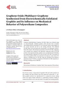
where ai;k,n (bi;k,n ) is the annihilation operator at momentum k and position n in sublattice Ai (Bi), i is the M n T layer index and Dk = −2 cos(k/2). The first term in OR B M eq. (1) describes in-plane hopping while the second term M n parametrizes the inter-layer coupling (t⊥ ≪ t). The symB bol • indicates a sum over non-balcony layers. Afterwards B n we consider the second nearest-neighbor interlayer hopimplies an extra Fig. 1: (a) Side and top views of bilayer graphene, and its two ping between A and B sublattices, P• Pwhich † −ik b ai∓1;k,n − term in eq. (1) given by −γ families of edge states: monolayer (M ) and bilayer (B ); the 3 i n i;k,n (e vertical axes represent the associated charge densities (squared e−ik/2 Dk ai∓1;k,n+1 ) + h.c., where γ3 ∼ t⊥ ≪ t. M
n
M
T
M
amplitudes). (b) Trilayer family of edge states (T ) occurring in trilayer graphene (vertical axes represent charge densities), and all other possible edge states (in schematic view). (c) Edge states in N -layer graphene (in schematic view).
some device applications [13–15]. Therefore, the question whether multilayer graphene possesses edge state physics is of paramount importance. In this Letter we show that zero energy states localized at zigzag edges do exist in multilayer graphene. Using the simplest first nearest-neighbor tight-binding model, we derive the analytical expression for multilayer graphene edge states and show that their number is always equal to the number of layers occurring at the edge. The effect of second nearest-neighbor interlayer hopping is considered, and the robustness of multilayer graphene edge states is shown. Finally, we generalize the edge state solution to graphite steps, where experimental evidence for edge states has been widely reported [3]. The theoretical solution given in this Letter agrees well with experimental findings. Also, we predict that edge states in graphite steps should be seen in scanning tunneling microscopy (STM) even when the step occurs underneath the first graphite layer.
Edge states in N -layer graphene. – Multilayer graphene edge states are investigated by solving the Schr¨odinger equation, Hk |ψk i = Ek |ψk i. The wavefunction |ψk i is written as a linear combination of the site amplitudes P P along the edge’s perpendicular direction, |ψk i = n i [αi (k, n) |ai , k, ni+βi (k, n) |bi , k, ni], where we have introduced the one-particle states |ci , k, ni = c†i;k,n |0i, with ci = ai , bi . In addition we require the boundary conditions αi (k, n → ∞) = αi (k, −1) = βi (k, n → ∞) = βi (k, −1) = 0, accounting for the existence of the edge at n = 0. Within our model, the Fermi energy of multilayer graphene always occurs at zero energy. Therefore, we expect zero energy edge states to have interesting physical consequences, and we set Ek = 0. As a result, the two sublattices become completely decoupled, and only the sublattice to which edge atoms belong can support edge states.1 This means that we always have βi (k, n) = 0. It was recently shown [17] that bilayer graphene supports two types of zero energy edge states localized at zigzag edges for 2π/3 < k < 4π/3: one type restricted to the balcony layer and coined monolayer family, with amplitudes equivalent to edge states in single layer graphene, k
α2 (k, n) = α2 (k, 0)Dkn e−i 2 n ;
(2)
and a new type coined bilayer family, with finite ampliModel. – We model AB-stacked multilayer graphene tudes over the two layers, as shown in fig. 1(a) (for the simplest case of a bilayer), n −i k 2n , where non-interacting π-electrons are allowed to hop only α1 (k, n) = α1 (k, 0)Dk e � Dk2 � k t⊥ between A and B sublattices. In what follows we use , α2 (k, n) = −α1 (k, 0)Dkn−1 e−i 2 (n−1) n − the terminology balcony layers for layers represented with t 1 − Dk2 dashed (red) lines, and non-balcony layers for those rep(3) resented with full (black) lines. Without loss of generality we assume all edge atoms belong to the A sublat- where the normalization constants are given by tice. The zigzag edge breaks translational invariance along |α2 (k, 0)|2 = 1 − Dk2 and |α1 (k, 0)|2 = (1 − Dk2 )3 /[(1 − its perpendicular direction, enabling us to write an effec1 In the ribbon geometry the two sublattices are equivalent, suptive one-dimensional Hamiltonian for a given momentum porting edge states localized in opposite ribbon edges. In the semi−1 k ∈ [0, 2π[ along the edge (in units of a ). The first infinite system, only those localized in the edge sublattice survive nearest-neighbor tight-binding Hamiltonian can be writ- [16, 17]. p-2
Surface states in multilayer graphene and graphite Dk2 )2 + t2⊥ /t2 ]. The charge densities (squared amplitudes) associated with the two families of edge states are represented in fig. 1(a). Let us now consider a trilayer as shown in fig. 1(b), where a non-balcony layer is sandwiched between two balcony layers. Clearly, the bilayer family is not an edge state solution for this trilayer, as any finite amplitude at a non-balcony layer implies, through eq. (1), a finite amplitude over adjacent layers. We note, however, that our model ignores the coupling between next nearest-layers.2 Thus, if we construct a trilayer wavefunction whose amplitudes over balcony/non-balcony layers mimic those for the bilayer family, it is guaranteed, apart from a normalization factor, that we have an edge state solution. More precisely, we arrive at a new type of edge state with finite amplitudes over three consecutive layers – trilayer family – whose analytic form can be written as Dk2 � t⊥ −i k (n−1) � , e 2 n− t 1 − Dk2
α1 (k, n) =
−α2 (k, 0)Dkn−1
α2 (k, n) =
α2 (k, 0)Dkn e−i 2 n , � t⊥ Dk2 � −α2 (k, 0)Dkn−1 e−i2)(n−1) n − , t 1 − Dk2 (4)
α3 (k, n) =
k
where the normalization constant is given by |α2 (k, 0)|2 = (1−Dk2 )3 /[(1−Dk2 )2 +2t2⊥ /t2 ]. The charge density (squared amplitude) associated with the trilayer family of edge states is represented in fig. 1(b). Additionally, the trilayer we have been discussing also supports edge states of the monolayer family localized at balcony layers, as schematically shown in fig. 1(b). In fact, this is a general result. Balcony layers have an edge sublattice which is not connected through t⊥ to adjacent layers. Thus, the monolayer family is always an edge state solution in N -layer graphene. Even more generally, we can look at a balcony layer as a buffer layer. As can be seen from eq. (1), a finite amplitude over a balcony layer does not imply finite amplitudes over adjacent layers. For the trilayer shown at the bottom of fig. 1(b), where a balcony layer is sandwiched between two non-balcony layers, monolayer edge states certainly exist at the middle balcony layer. But because of the buffer layer character, also bilayer edge states are present, localized either at the two top or the two bottom layers. An immediate consequence of the buffer layer concept is the fact that the trilayer family is the most general edge state family we can have, and exists localized at any non-balcony layer and its two adjacent layers, with all other site amplitudes equal to zero. Therefore, we have three families of edge states occurring in multilayer graphene: (i) monolayer family for each balcony layer, eq. (2); (ii) bilayer family for each non-balcony layer that starts and/or ends the multilayer, eq. (3); (iii) trilayer family for each non-balcony layer sandwiched be2 This is a reasonable approximation since in the SlonczewskiWeiss-McClure parametrization γ2 , γ5 ≪ t⊥ , γ3 [6].
tween two balcony ones, eq. (4). This is schematically represented in fig. 1(c). Note that the number of edge state families is always equal to the number of edge layers. Effect of γ3 . – In multilayer graphene the effect of γ3 is of the order of t⊥ , and should be included in a consistent edge state solution. The buffer layer concept introduced previously, however, does not survive at a finite γ3 . In order to generalize the edge state solution to the present case we use the transfer matrix technique, following ref. [17]. For bilayer graphene the transfer matrix, defined as [α1 (k, n), α2 (k, n)]T = e−ikn/2 T(2)n [α1 (k, 0), α2 (k, 0)]T , is given by � � u v , (5) T(2) = x Dk where u = Dk (1 − ξ), v = − γt3 e−ik/2 (1 − Dk2 ), and x = − tt⊥ eik/2 , with ξ = t⊥ γ3 /t2 . The edge states are completely determined by the eigenvalues λ± and eigenvectors χ± of the transfer matrix. If |λ± | < 1, then edge states exist and are given by [α1 (k, n), α2 (k, n)]T ∝ e−ikn/2 λn± χ± , apart from a normalization constant.√Diagonalizing eq. (5) p we obtain λ± = Dk (1 − ξ/2) ± ξ Dk2 (ξ/4 − 1) + 1. Simple algebra shows√that for λ+ the convergence condi−1 tion implies 2 cos−1 ( 1 + ξ/2) √ < k < 2 cos [−(1 − ξ)/2] −1 or 4π/3 < k < √ 2 cos (− 1 + ξ/2), while for−1λ− it implies 2 cos−1 ( 1 + ξ/2) √ < k < 2π/3 or 2 cos [(1 − ξ)/2] < k < 2 cos−1 (− 1 + ξ/2). We conclude that bilayer graphene still has two families of edge states for γ3 6= 0, though the k range is slightly changed when compared with the γ3 = 0 case. In particular, we have only one family for k ∈ [2π/3, 2 cos−1 [(1 − ξ)/2]] and k ∈ [2 cos−1 [−(1 − ξ)/2], 4π/3], although the existence of edge states for k < 2π/3 and k > 4π/3 compensates this reduction, and we still have edge states for 1/3 of the possible k’s, as in the γ3 = 0. As a test to what has just been said, we have numerically computed the energy spectrum for a bilayer ribbon with zigzag edges (t⊥ = γ3 = 0.2t and width 400 unit cells). The result is shown in fig. 2(a). Four flat bands at zero energy are clearly seen, and can be identified with the abovementioned two families of edge states, two per edge. The insets reveal the k restrictions mentioned before. In fact, the values of k that limit the existence or number of edge states coincide with the Dirac points and satellite Fermi points that arise when γ3 6= 0 [18], as indicated by the thin red lines (the mismatch is due to the finite width of the ribbon, and consequent edge state overlap). The transfer matrix eigenvectors can be written as χ± = [λ± −Dk , − tt⊥ eik/2 ]T , from which P we can write two families of wavefunctions, ∞ |ψ± i = C± n=0 e−ikn/2 λn± χ± , where the normalization constant is given by C± = [(1 − |λ± |2 )/(|λ± − Dk |2 + t2⊥ /t2 )]1/2 . Note, however, that χ+ and χ− are not orthogonal, implying the non-orthogonality of the two solutions |ψ± i. It is convenient to orthogonalize |ψ− i with respect to |ψ+ i, whose result can be written as |ψ˜− i = (|ψ− i − hψ+ |ψ− i|ψ+ i)/(1 − |hψ+ |ψ− i|2 ), where hψ+ |ψ− i = C+ C− (t2⊥ /t + ξDk2 − ξ)/(1 − Dk2 + ξ). In
p-3
E. V. Castro et al. (a) 0.2
0.32
(b)
0.34
0.05
0.01
0.1
0
γ3 = 0.01t
M
0
γ3 = 0.1t
E/t
-0.01
0.05
0
0.64
0.66
0.68
0
0.01
-0.1
0
γ3 = 0.2t
0.05
-0.01
-0.2
B
0.3
0.4
0.5
k/2π
0.6
0.7
0
0
|α1(k,n)|
2
20 40 60 0
n
|α2(k,n)|
2
20 40 60
n
Fig. 2: (a) Energy spectrum for a bilayer ribbon with zigzag edges at finite γ3 . (b) Charge density for bilayer graphene edge states, monolayer (M ) and bilayer (B ) families, at k/2π = 0.35. Thin lines show the γ3 = 0 result.
Fig. 3: Number of edge states per layer in N -layer graphene as a function of k: (a) γ3 = 0; (b) γ3 = t⊥ ; (c) γ3 = 2t⊥ . We set t⊥ = 0.2t.
Graphite steps. – Finally, we generalize the edge state solution to graphite steps, where experimental evidence for edge states has been widely reported [3, 22–28]. fig. 2(b) we show the squared amplitudes associated with The local density of states (LDOS) peak seen in STM |ψ+ i (left) and |ψ˜− i (right). The thin lines represent the of graphite steps has been interpreted as the experimenedge states in bilayer graphene for γ3 = 0, as given by tal confirmation of the theoretically predicted single layer eqs. (2) and (3). Clearly, as long as γ3 ≪ t⊥ , we can edge states [29]. However, we can easily convince ouridentify |ψ+ i with the monolayer family and |ψ˜− i with selves that monolayer edge states do not always provide the bilayer family discussed previously. For γ3 ∼ t⊥ , the an eigenstate for a zigzag step-edge. To see why, we conedge state |ψ+ i, former monolayer family, already has an sider fig. 4(a), where the two possible zigzag step-edges on the surface of graphite are shown. These two terminations appreciable weight on both layers. The analysis made for bilayer graphene with γ3 6= are denoted α-type and β-type. For an α-type termina0 can be extended to N -layer graphene. Defin- tion the edge carbon atoms occur exactly on top of carbon ing the transfer matrix as [α1 (k, n), . . . , αN (k, n)]T = atoms of the underlying layer, while for a β-type termie−ikn/2 T(N )n [α1 (k, 0), . . . , αN (k, 0)]T , we can derive its nation they occur at the center of the hexagons. Obviously, monolayer edge states as given by eq. (2) cannot be general pattern for a given number of layers N , eigenstates for α-steps, as some finite amplitude must be induced on the second layer through eq. (1). For β-steps, u v −ξDk however, single layer edge states are indeed eigenstates. x D x k In order to have a step-edge we need at least two −ξDk v u v −ξDk . T(N ) = graphene layers. Indeed, step-edges are easily obtained x Dk x from bilayer graphene just by growing one of the layers be −ξDk v u ··· yond the edge. So, localized states at graphite steps can be .. .. . . understood by studying generalized bilayers where bottom (6) and top graphene layers have different widths. The two The periodic structure of T(N ) is readily identified, and families of edge states we have found to exist at zigzag the transfer matrix for any multilayer graphene is eas- edges of bilayer graphene remain eigenstates even when ily constructed. By diagonalizing eq. (6), and checking one of the layers is wider than the other. In particular, whether the eigenvalues λ satisfy |λ| < 1, we can conclude the solution given by eq. (2) and the non-orthogonalized about the existence of edge states in N -layer graphene for solution for edge states of the bilayer family given by γ3 6= 0. In fig. 3 the number of edge states per layer is shown in the plane number of layers (N ) vs k. Panel 3(a) k α1 (k, n) = α1 (k, 0)Dkn e−i 2 n , confirms what has been said for γ3 = 0: same number of k t⊥ edge states as the number of layers for 2π/3 < k < 4π/3. α2 (k, n) = −α1 (k, 0)nDkn−1 e−i 2 (n−1) , (7) t As shown in panels 3(b) and 3(c), around the Dirac points the number of edge states for γ3 6= 0 may be smaller than the number of layers, as we have seen for N = 2. How- [a simple linear combination of eqs. (2) and (3)], can be ever, there is always a broad region in between the Dirac adapted to the generalized bilayer just by adjusting the points where the number of edge states equals the num- unit cell index n. Then, Gram-Schmidt orthogonalization ber of layers. Thus, we conclude that multilayer graphene gives the final solution. We should note, however, that edges states are robust to second nearest-neighbor inter- the overlap between the two types of edge states is expolayer hopping. This result agrees with first principles cal- nentially suppressed as the difference in layer width gets culations, where the presence of edge states and edge mag- larger. When the width of one layer becomes infinite – the netism have been reported in bilayer [19, 20] and graphite case of a perfect step – only one of the two possible solu[21] zigzag nanoribbons. tions exists. Therefore, the possible localized solutions for p-4
Surface states in multilayer graphene and graphite α
β
(9)
amplitude. Consequently, we expect a similar asymmetry to be present in the LDOS peak induced by edge states at the Fermi level, which, ultimately, should be seen with STM. To better appreciate this effect, we have computed the LDOS of a generalized bilayer – bottom layer wider than the top layer – using the recursive Green’s function method [30]. The calculated LDOS, which was accumulated in the range 0.01t near the Fermi energy, should be proportional, in the simplest approximation, to the local tunnel currents in the experimental STM images [25, 31]. In fig. 4(c) we show, for the top layer (edge sublattice), the LDOS difference between β-type and α-type terminations as we move away from the step at n = 0. As expected, the LDOS at β-steps is higher and extends further into the bulk, a trend that is still present for realistic values of γ3 , as shown in fig. 4(c). This behavior agrees with STM results, where two types of edge states with different penetration depths have been seen [26]. Edge states with reduced penetration depth have been observed at α-type steps, whereas at β-type steps the edge states extend further into the bulk, as we have obtained here for the top layer component. However, right at the edge, the STM intensity has been found to be higher at α-steps than βsteps [26]. According to our analytical result the opposite should be seen. This discrepancy is most probably due to edge state admixture, as experimentally both α-type and β-type steps coexist on the same step-edge. In fig. 4(d) and 4(e) we show the top layer LDOS map for α- and β-steps, respectively. The former presents not only a reduced penetration depth, as previously discussed, but also higher intensity at sites connected to the underlying layer through t⊥ , as opposed to standard LDOS maps on the surface of bilayer graphene and graphite. This behavior is characteristic of edge states at α-type steps, as given by eq. (8). fig. 4(f) and 4(g) show the underlying layer LDOS map for α- and β-steps, respectively. As edge states at α-steps [eq. (8)] have a finite amplitude over the underlying layer, the LDOS map for this layer shows an increased intensity at and near the step [fig. 4(f)], although the lattice discontinuity only exists at the other layer. As a consequence, we expect α-steps to be detected in STM experiments even when they occur underneath the top layer. This feature is not seen in β-type steps [fig. 4(g)].
for a β-type step, where n ≥ 0 and the normalization constant in eq. (8) is given by |Ck |2 = (1 − Dk2 )3 /[(1 − Dk2 )2 + (1 + Dk2 )t2⊥ /t2 ]. As in edge states discussed previously, the amplitudes in eqs. (8) and (9) refer to sites belonging to the same sublattice as the edge carbon atoms, while the amplitudes at the other sublattice are zero. Example charge densities for the given edge states are shown in fig. 4(b) for both the α-type and the β-type step-edges. As can be seen from eqs. (8) and (9), or by inspection of fig. 4(b), there is an apparent asymmetry between the two families of edge states: edge states at β-type steps live only on the top layer, while at α-type steps both the top layer and the underlying layer have a finite edge state
Conclusions. – We have demonstrated the existence of zero energy states localized at zigzag edges of multilayer graphene and graphite steps. Stability to the presence of interlayer hopping γ3 has been shown. The electron-hole symmetry breaking terms γ4 (interlayer) and t′ (inplane) are expected to induce edge state dispersion, but not to qualitatively modify the present results [32, 33]. It should be noted that only perfect zigzag edges have been discussed here. However, we expect edge state properties to be present in multilayer graphene and graphite steps even for irregular edges, as long as some zigzag units are present, as recently demonstrated for single layer graphene [34, 35]. On the other hand, zigzag edges have been re-
(b) 0.1
0
α - step
β - step
top bottom
0 10 20 30 40
n
(c)
top
0 10 20 30 40
n
LDOS(β) − LDOS(α)
LDOS (arb. units)
(a)
γ3 = 0 γ3 = 0.05t γ3 = 0.1t
0 1 2 3 4 5 6 7 8 9
n
Fig. 4: (a) Possible zigzag steps on graphite’s surface. (b) Charge density for edge states at α-type and β-type stepedges (ka/2π = 0.35). (c) LDOS difference between β- and α-type steps as a function of n. (d)-(e) Top layer LDOS map for α- and β-steps, respectively. (f)-(g) Underlying layer LDOS map for α- and β-steps, respectively. We set t⊥ = 0.1t.
zigzag step-edges (occurring at n = 0) are: αtop (k, n) αbottom (k, n)
k
= Ck Dkn e−i 2 n , k t⊥ = −Ck nDkn−1 e−i 2 (n−1) , t
(8)
for an α-type step, and k
αtop (k, n) = (1 − Dk2 )Dkn e−i 2 n ,
p-5
E. V. Castro et al. cently observed in epitaxial graphene monolayer [36], providing the first indication that edge shape can be a controllable parameter in the future. Our findings are relevant in the context of carbon based magnetism, where edge states seem to play an important role [1, 3], and also in the context of graphene physics, where the reported self-doping in monolayer graphene [36] and suppression of conductance fluctuations near the neutrality point in bilayer and trilayer graphene [37] can be seen as edge states driven effects. ∗∗∗ E.V.C., N.M.R.P., and J.M.B.L.S. acknowledge financial support from POCI 2010 via project PTDC/FIS/64404/2006. REFERENCES [1] Makarova T. and Palacio F., (Editors) Carbon Based Magnetism (Elsevier, Amsterdam) 2006. [2] Enoki T. and Kobayashi Y., J. Mater. Chem. , 15 (2005) 3999 . [3] Enoki T., Kobayashi Y. and Fukui K., Int. Rev. Phys. Chem. , 26 (2007) 609. [4] Geim A. K. and Novoselov K. S., Nat. Mater. , 6 (2007) 183. [5] Katsnelson M. I., Mater. Today , 10 (2007) 20. [6] Castro Neto A. H., Guinea F., Peres N. M. R., Novoselov K. S. and Geim A. K., The electronic properties of graphene arXiv:0709.1163 (to appear in Rev. Mod. Phys.). [7] Kopelevich Y. and Esquinazi P., J. Low Temp. Phys. , 146 (2007) 629. ¨ hne R., Spemann D., [8] Ohldag H., Tyliszczak T., Ho Esquinazi P., Ungureanu M. and Butz T., Phys. Rev. Lett. , 98 (2007) 187204. [9] Pereira V. M., Guinea F., Lopes dos Santos J. M. B., Peres N. M. R. and Castro Neto A. H., Phys. Rev. Lett. , 96 (2006) 036801. [10] Wakabayashi K., Electronic and magnetic properties of nanographite in Carbon Based Magnetism, edited by Makarova T. and Palacio F., (Elsevier, Amsterdam) 2006 Ch. 12 pp. 279–304. [11] Lehtinen P. O., Foster A. S., Ma Y., Krasheninnikov A. V. and Nieminen R. M., Phys. Rev. Lett. , 93 (2004) 187202. [12] Son Y.-W., Cohen M. L. and Louie S. G., Nature , 444 (2006) 347. [13] Castro E. V., Novoselov K. S., Morozov S. V., Peres N. M. R., Lopes dos Santos J. M. B., Nilsson J., Guinea F., Geim A. K. and Castro Neto A. H., Phys. Rev. Lett. , 99 (2007) 216802. [14] Oostinga J. B., Heersche H. B., Liu X., Morpurgo A. F. and Vandersypen L. M. K., Nat. Mater. , 7 (2008) 151 . [15] Lin Y.-M. and Avouris P., Nano Lett. , 8 (2008) 2119. [16] Wakabayashi K., Fujita M., Ajiki H. and Sigrist M., Phys. Rev. B , 59 (1999) 8271.
[17] Castro E. V., Peres N. M. R., Lopes dos Santos J. M. B., Castro Neto A. H. and Guinea F., Phys. Rev. Lett. , 100 (2008) 026802. [18] McCann E. and Fal’ko V. I., Phys. Rev. Lett. , 96 (2006) 086805. [19] Lee H., Son Y.-W., Park N., Han S. and Yu J., Phys. Rev. B , 72 (2005) 174431. [20] Sahu B., Min H., MacDonald A. H. and Banerjee S. K., Phys. Rev. B , 78 (2008) 045404. [21] Miyamoto Y., Nakada K. and Fujita M., Phys. Rev. B , 59 (1999) 9858 . [22] Klusek Z., Waqar Z., Denisov E. A., Kompaniets T. N., Makarenko I. V., Titkov A. N. and Bhatti A. S., Appl. Surf. Sci. , 508 (2000) 161. [23] Niimi Y., Matsui T., Kambara H., Tagami K., Tsukada M. and Fukuyama H., Appl. Surf. Sci. , 241 (2005) 43. [24] Kobayashi Y., ichi Fukui K., Enoki T., Kusakabe K. and Kaburagi Y., Phys. Rev. B , 71 (2005) 193406. [25] Niimi Y., Matsui T., Kambara H., Tagami K., Tsukada M. and Fukuyama H., Phys. Rev. B , 73 (2006) 085421. [26] Kobayashi Y., Fukui K., Enoki T. and Kusakabe K., Phys. Rev. B , 73 (2006) 125415. [27] Banerjee S., Sardar M., Gayathri N., Tyagi A. K. and Raj B., Appl. Phys. Lett. , 88 (2006) 062111. [28] Sugawara K., Sato T., Souma S., Takahashi T. and Suematsu H., Phys. Rev. B , 73 (2006) 045124. [29] Fujita M., Wakabayashi K., Nakada K. and Kusakabe K., J. Phys. Soc. Jpn. , 65 (1996) 1920. [30] Haydock R., The recursive solution of the schr¨ odinger equation in Solid State Physics, edited by Ehrenreich H., Seitz F. and Turnbull D., Vol. 35 (Academic Press, New York) 1980 p. 215. [31] Tersoff J. and Hamann D. R., Phys. Rev. B , 31 (1985) 805 . [32] Peres N. M. R., Guinea F. and Castro Neto A. H., Phys. Rev. B , 73 (2006) 125411. [33] Sasaki K., Murakami S. and Saito R., Appl. Phys. Lett. , 88 (2006) 113110. [34] Kumazaki H. and Hirashima D. S., J. Phys. Soc. Jpn. , 77 (2008) 044705. [35] Bhowmick S. and Shenoy V. B., J. Chem. Phys. , 128 (2008) 244717. [36] de Parga A. L. V., Calleja F., Borca B., Jr M. C. G. P., Hinarejo J. J., Guinea F. and Miranda R., Phys. Rev. Lett. , 100 (2008) 056807. [37] Staley N. E., Puls C. and Liu Y., Phys. Rev. B , 77 (2008) 155429.
p-6