Hindawi Publishing Corporation Journal of Sensors Volume 2016, Article ID 1740854, 15 pages http://dx.doi.org/10.1155/2016/1740854
Research Article Low-Cost Monitoring System of Sensors for Evaluating Dynamic Solicitations of Semitrailer Structure Pablo Luque,1 Daniel A. Mántaras,1 Aida Rodríguez,1 Hugo Malón,2 Luis Castejón,2 Javier G. Jalón,3 José L. López,3 and Ángel Martín3 1
Escuela Polit´ecnica de Ingenier´ıa de Gij´on, Universidad de Oviedo, Campus de Gij´on, s/n, Gij´on, 33203 Asturias, Spain Departamento de Ingenier´ıa Mec´anica, Universidad de Zaragoza, c/Mar´ıa de Luna, s/n, 50018 Zaragoza, Spain 3 Universidad Polit´ecnica de Madrid, INSIA, Campus Sur UPM, Carretera de Valencia (A-3), km 7, 28031 Madrid, Spain 2
Correspondence should be addressed to Pablo Luque;
[email protected] and Hugo Mal´on;
[email protected] Received 6 January 2016; Revised 13 October 2016; Accepted 17 October 2016 Academic Editor: Andrea Cusano Copyright © 2016 Pablo Luque et al. This is an open access article distributed under the Creative Commons Attribution License, which permits unrestricted use, distribution, and reproduction in any medium, provided the original work is properly cited. Analysis of the fatigue life of a semitrailer structure necessitates identification of the loads and dynamic solicitations in the structure. These forces can be introduced in computer simulation software (multibody + finite element) for analysing the response of different design solutions to them. These numerical models must be validated and some parameters need to be measured directly in a field test with real vehicles under various driving conditions. In this study, a low-cost monitoring system is developed for application to a real fleet of semitrailers. According to the definition of the numerical model, the guidance of a virtual vehicle is defined by the three-dimensional kinematics of the kingpin. For characterisation of these movements, a monitoring system having a lowcost inertial measurement unit (IMU) and global positioning system (GPS) antennas is developed with different configurations to enable analysis of the best cost-benefit (result accuracy) solution, and an extended Kalman filter (EKF) that characterises the kinematic guidance of the kingpin is proposed. A semitrailer was equipped with the experimental low-cost monitoring system and high-precision sensors (IMU, GPS) in order to validate the results obtained by the experimental low-cost monitoring system and the inertial-extended Kalman filter developed. The validated system has applicability in the low-cost monitoring of a fleet of real vehicles.
1. Introduction Vehicle weight reduction is one of the effective approaches for reducing fuel consumption and emissions [1]. A simulation has revealed that, for every 10% weight reduction from the weights of an average new car and light truck, their fuel consumption would reduce by 6.9% and 7.6%, respectively. In the case of a commercial vehicle, a reduction in its kerb weight corresponds to an increased payload capacity. Therefore, weight reduction has a greater impact for this type of vehicle than for other types of vehicles. In semitrailers, the body frame represents more than 75% of the total weight; therefore, this component has the most room for improvement. Weight reduction of the body frame should be achieved while keeping the safety level of the
vehicle and the ability of the vehicle and of its components to maintain their functions unchanged or while limiting the vehicle’s degradation with aging to acceptable levels. Today, for heavy-duty trucks, an adequate endurance specification is assumed when 10% of the population of vehicles produced exceed the 800,000 km without any failure [2]. Phenomena that can influence the endurance of a vehicle can be classified into the following categories: fatigue, wear, corrosion, and shocks and collisions. Weight reduction of the body frame of a vehicle affects its fatigue life; therefore, to ensure that the aging and endurance remain unaffected by this reduction, it is necessary to establish the vehicle design on the basis of a detailed study of the fatigue life. Fatigue life evaluation necessitates an accurate identification of the loads that the body frame
2
Journal of Sensors
Testing low-cost sensor Kingpin kinematic CAE, multibody dynamics simulation with flexible body (MSC-AdamsANSYS/ABAQUS)
Optimized design
Loads
Fatigue analysis S, Mises Envelope (max. abs.) (avg.: 75%) +3.561e + 02 +3.265e + 02 +2.968e + 02 +2.671e + 02 +2.374e + 02 +2.078e + 02 +1.781e + 02 +1.484e + 02 +1.187e + 02 +8.905e + 01 +5.937e + 01 +2.969e + 01 +1.163e − 02 S, Mises Envelope (max. abs.) (avg.: 75%) +3.595e + 02 +3.296e + 02 +2.996e + 02 +2.696e + 02 +2.397e + 02 +2.097e + 02 +1.798e + 02 +1.498e + 02 +1.198e + 02 +8.989e + 01 +5.993e + 01 +2.997e + 01 +9.629e − 03
Figure 1: Methodology for fatigue life calculation.
will be subjected to during operation and performance of optimization by the use of simulation techniques based on the Finite Element Method. The methodology for fatigue life calculation is established by means of a virtual test, as shown in Figure 1. As shown in this figure, a real vehicle is employed for performing discretisation of the body frame by means of finite element software (such as ANSYS or ABAQUS). This chassis information is then introduced in multibody dynamics simulation software (such as ADAMS of MSC Software Co.) to develop a virtual experimental program. This program includes different driving conditions (speed, manoeuvres, obstacles, roads, etc.) with the aim of defining the load cases to be introduced in fatigue life prediction algorithms. To determine the loads during vehicle operation, a methodology based on the simulation of virtual models using data acquired by low-cost instrumentation has been developed. The effectiveness of this methodology—which combines acquired real data and a virtual model to optimise designs—for application to other types of vehicles has been proved [3]. The main advantage of combining a virtual model and real data is the reduction in the complexity of the data acquisition system and the required number of sensors. In a vehicle such as that analysed, the loads necessary for
calculation of the fatigue life are due to the actions of tractor, suspension, load, and so forth [4, 5]. This implies the need for complex instrumentation, thereby making this methodology unsuitable for application to a vehicle fleet. The present paper presents the development and implementation of a low-cost instrumentation system that is nonintrusive and robust; this system was developed with the aim of applying the above-described methodology to trailertype vehicles. A semitrailer is a vehicle that can be coupled to different tractor vehicles. Therefore, in order for the virtual model to be able to calculate the loads regardless of which tractor vehicle is connected to the semitrailer, the inputs to the virtual model are proposed to be the actions of the tractor vehicle at the point of connection. The multibody model inputs developed for use with the methodology can be forces, acceleration, velocities, and/or positions. Given the need to develop a low-cost system to provide inputs to the model, the kinematic guidance of the connection point (i.e., kingpin) between the tractor and the semitrailer was selected as the input in the present study.
2. Materials and Methods 2.1. Related Work. The most appropriate device for measuring the velocity of the kingpin is a Global Navigation
Journal of Sensors
3
45
(ii) Extended temporal coverage: one sensor is able to detect or measure an event at times when the other sensors are unable to.
40 35
(iii) Extended spatial coverage: one sensor can cover what other sensors cannot.
(km/h)
30 25
(iv) Increased confidence: multiple independent measurements provide information on the same event.
20 15
(v) Improved detection performance: multiple independent measurements of the same event are integrated effectively.
10 5 0 0
200
400
600
800
1000
1200
1400
(Meters)
Figure 2: Variations in measured velocity due to noise in GNSS in actual test.
Satellite System (GNSS) receiver, because two of the outputs are the absolute speed and the course angle (as of April 2013, only the United States NAVSTAR global positioning system (GPS) and the Russian GLONASS were global operational GNSSs). However, the velocity acquired with a low-cost GNSS receiver causes two problems—a high level of noise and low precision, which worsen under the influence of external factors such as multipath and low satellite visibility [8]. Given the environment in which these vehicles operate, these problems occur frequently. Noise in the GNSS signal implies variations in the measured velocity, which in turn implies significant changes in acceleration (Figure 2). During simulation, these variations in the input of the virtual model translate into loads much higher than actual loads. Fatigue analysis based on thus obtained loads would be unreliable, and filtering of the input signal would not solve this problem. Furthermore, speed measurement of the kingpin using a GNSS receiver cannot be performed for all types of vehicles, since the kingpin is usually hidden under the box or the load, and this approach is applicable only in the case of a semitrailer or container. In consideration of both of these problems, the low-cost system developed in the present study is equipped with an inertial filter—specifically, an inertial-extended Kalman filter (i-EKF)—for the estimation of velocity of the kingpin using a GNSS receiver, which can be placed at a different location. The proposed low-cost system is based on the concept of fusion of an inertial measurement unit (IMU) and GNSS receivers with low-cost sensors. Sensor fusion refers to the combination of data acquired from multiple sensors with related information, which facilitates achievement of more specific inferences than those possible by using a single independent sensor [9]. The following are the advantages of using a multisensor approach over a single-sensor approach [10]: (i) Robust operational performance: any of the sensors has the potential to provide information during unavailability malfunctioning or failure of the other sensors.
(vi) Reduced vulnerability to denial: this occurs as a result of increased dimensionality of the measurement space. The following are the advantages of sensor-fused data over single-sensor data [9]: (i) Improved estimate: if several identical sensors are used, combination of observations from these sensors may lead to an improved estimate. Furthermore, a statistical advantage is gained by the addition of independent observations, under the assumption that the data are combined in an optimal manner. (ii) Improved observation process: use of the relative placement or motion of multiple sensors may result in an improved observation process. For example, two sensors that measure the angular directions to an object can be coordinated to determine the position of the object via triangulation. (iii) Improved observability: broadening of the baseline of physical observables can result in significant improvements. If the observations are associated correctly, the combination of sensors provides a better estimation than what could be obtained by any of the sensors independently. This results in a smaller error region. The fusion of an IMU and GNSS receiver is frequently used for accurate determination of attitude. In [11], with the aim of determining the full attitude even for a nonaccelerating vehicle, a navigation system that incorporates inertial and two-antenna carrier phase differential GPS measurements was developed. Aided inertial navigation is a well-studied problem [12–16]. Several GPS pseudorange and Doppleraided inertial systems have been documented in the literature; see, for example, [17]. A low-cost system that fuses inertial sensing and a twoantenna GPS with an unscented Kalman filter (UKF) has been developed in [18]. Many previous works on low-cost attitude estimation [19–28] have focused on the fusion of inexpensive sensors, including microelectromechanical system(MEMS-) based gyroscopes and accelerometers, magnetometers, and the GPS. In low-cost land vehicle navigation applications, in addition to accurate position and velocity information being required, an accurate attitude needs to be provided by the navigation system [28–31]. Use of the GPS signal for attitude determination has several advantages such as the small size, low cost, lack of cumulative errors, and high accuracy of
4 the GPS. However, attitude determination using the GPS also has drawbacks such as its susceptibility to the external environment and instability in dynamic applications [31]. The conventional method of attitude determination is to use an inertial navigation system (INS). However, the INS has a drawback in that errors accumulate over time, especially in the case of a low-cost MEMS-INS. If the GPS and MEMSINS are combined effectively, the reliability and accuracy of attitude determination can be improved [32–34]. The low-cost system proposed in this work differs from conventional systems in that it entails estimation of the velocities (to be used as inputs in computer simulation models) at a point of the vehicle and not the position or attitude. In any case, given the advantages of the fusion of these sensors, estimation of other states that are inputs to safety systems is a routine methodology for a vehicle. Several works have proposed estimation methods of several key vehicle states—sideslip angle, longitudinal velocity, roll, and grade—for example, by combining automotivegrade inertial sensors with a GPS receiver [35]. Kinematic estimators that are independent of uncertain vehicle parameters integrate inertial sensors with GPS antennas to provide high update estimates of the vehicle states and sensor biases. Use of a two-antenna GPS system would enable quantification of the effects of pitch and roll on the measurements, which have been demonstrated to be quite significant in sideslip angle estimation. The sideslip angle is an important state of vehicle lateral dynamics, and its estimation has been studied by many researchers [36–45]. For example, Bevly et al. proposed an estimation method that utilises a single-antenna GPS along with an IMU [43, 44]. This method essentially integrates the bias-corrected yaw rate to obtain the vehicle heading angle, which can provide the sideslip angle along with the vehicle velocity angle measured by the single-antenna GPS. In [46], a new method was proposed that employs two low-cost singleantenna GPS receivers to estimate the vehicle sideslip angle. In the present study, four kinematics equations that relate the velocities of two different GPS receivers to the heading angle and to the longitudinal/lateral velocities of a vehicle are presented. These equations are then analysed in order to determine the theoretical limit of the sideslip/heading angle estimation. Fusion of a GPS with an IMU through an EKF is performed. 2.2. Mathematical Model. A mathematical model of a semitrailer is established in this section. This model is then used in a computer simulation to implement an EKF with a low-cost IMU and GPS receivers. According to the definition of the mathematical model, the longitudinal and lateral acceleration values (vehicle frame) and the yaw rate provided by the IMU are used as inputs. The GPS speed (reference frame) is considered as an output or measurement vector. 2.2.1. Reference and Vehicle Frames. For the definition of the vehicle dynamics model and computer simulation model, the kinematics of the kingpin should be defined as an input by characterising its speed. According to the usual approach
Journal of Sensors of using a multibody system, it is necessary to define the kinematics in local coordinates in accord with the motion of the vehicle. Given that the employed sensing system includes various types of sensors, two reference systems are defined. Reference Frame. The following is the notation of coordinates used for the reference frame (sometimes termed the local vertical, local horizontal (LVLH) frame): east, north, up (ENU). The local ENU coordinates are formed from a plane tangential to the Earth’s surface, fixed at a specific location; therefore, this plane is sometimes known as a “local tangent” or “local geodetic” plane. Vehicle Frame. In this case, the sensitive axes of the accelerometer sensor are made to coincide with the axes of the semitrailer. The origin coincides with the location of the kingpin of the vehicle. This frame is in accordance with the ISO standards, specifically ISO 8855. In this coordinate system (Figure 3), the forward movement of the vehicle is described along the positive x-axis; the lateral movement of the vehicle is described along the y-axis; it is positive when the vehicle is oriented to the left (from the driver’s position); and the vertical movement of the vehicle is described along the z-axis. 2.2.2. Extended Kalman Filter. In order to apply the proposed methodology, the equations of the virtual model must be expressed in space-state form. The state-space representation of a physical system is composed of a set of inputs, outputs, and state variables related via first-order differential equations, which are combined in a first-order matrix differential equation. The state variables or states are expressed as vectors and the algebraic equations are written in matrix form, provided that it is a linear system. A general way to represent a nonlinear system with 𝑝 inputs, 𝑞 outputs, and 𝑛 states is as follows: 𝑥̇ (𝑡) = f (𝑡, 𝑥 (𝑡) , 𝑢 (𝑡) , 𝑤 (𝑡)) , 𝑦 (𝑡) = h (𝑡, 𝑥 (𝑡) , 𝑢 (𝑡) , V (𝑡)) .
(1)
Here, the first equation is the state equation and the second one is the output equation, where 𝑥(𝑡) is the “state vector,” 𝑥(𝑡) ∈ R3 ; 𝑢(𝑡) is the “input vector,” 𝑢(𝑡) ∈ R3 ; 𝑦(𝑡) is the “output vector,” 𝑦(𝑡) ∈ R𝑞 ; and 𝑤(𝑡) and V(𝑡) are random variables that represent the process noise and measurement noise, respectively. Applying the concept of Taylor series expansion, the estimation around the current estimate can be linearised using the partial derivatives of the process and the measurement functions in order to compute estimates even in the face of nonlinear relationships. It can be assumed that the system has a state vector 𝑥(𝑡) ∈ R𝑛 and that it is governed by the nonlinear stochastic difference equation. In discrete form, the equation can be expressed as 𝑥 (𝑘) = f (𝑥 (𝑘 − 1) , 𝑢 (𝑘 − 1) , 𝑤 (𝑘 − 1)) , 𝑦 (𝑘) = h (𝑥 (𝑘) , 𝑢 (𝑘) , V (𝑘)) ,
(2)
Journal of Sensors
5
x 𝛽 Vehicle frame (x, y) VKP
y
𝜓
𝜐KP
Vx_KP
Vy_KP KP
Reference frame (E, N)
N (north)
E (east)
Figure 3: Reference and vehicle frames.
where the measurement equation is 𝑦 (𝑘) = h (𝑥 (𝑘) , 𝑢 (𝑘) , V (𝑘)) .
(3)
In this case, the nonlinear function “f” is the difference equation that relates the state at the previous time step (𝑘 − 1) to that at the current time step (k). The state vector (𝑥(𝑡) ∈ R3 ) is defined as follows: 𝑥1 (𝑘) 𝑉𝑥 KP (𝑘) [𝑥 ] [𝑉 ] 𝑥 (𝑘) = [ 2 (𝑘)] = [ 𝑦 KP (𝑘)] . [𝑥3 (𝑘)]
(4)
[ 𝜓 (𝑘) ]
[𝑢3 (𝑘)]
(5)
[ 𝜓̇ (𝑘) ]
𝑤(𝑡), which represents the process and measurement noises, is given as 𝜂𝑉𝑥 KP 𝑤1 (𝑘) ] ] [ [𝑤 ] 𝑤 (𝑘) = [ 2 (𝑘)] = [ [𝜂𝑉𝑦 KP ] . [𝑤3 (𝑘)]
[ 𝜂𝜓 ]
̃ (𝑘) = f (̂ 𝑥 𝑥 (𝑘 − 1) , 𝑢 (𝑘 − 1) , 0) , ̃ (𝑘) = h (̃ 𝑦 𝑥 (𝑘) , 𝑢 (𝑘) , 0) ,
Further, 𝑢(𝑡) ∈ R3 , which represents the inputs from the IMU (acceleration and yaw rate), is expressed as 𝑢1 (𝑘) 𝑎𝑥 KP (𝑘) [𝑢 ] [𝑎 ] 𝑢 (𝑘) = [ 2 (𝑘)] = [ 𝑦 KP (𝑘)] .
Finally, 𝑦(𝑡) represents the “output vector” and 𝑦(𝑡) ∈ R𝑞 . Its value is obtained via different study cases and it depends on the adopted instrumentation system and layout, as described later. In practice, the individual values of the noises 𝑤(𝑘 − 1) and V(𝑘 − 1) at each time step are unknown. However, the state and measurement vectors without these values can be, respectively, approximated as
(6)
(7)
̃ (𝑘) is some a posteriori estimate of the state (from a where 𝑥 previous time step 𝑘). 2.2.3. Development of the Mathematical Model of Semitrailer Using i-EKF. It is considered that the vehicle (semitrailer) performs a flat movement and that it is guided by the tractor unit (truck), as described in Figure 3. The implemented vehicular dynamics model takes into account the inertial effects, but it does not consider dynamic roll, suspension performance, inclination of the road, and so forth. For the formulation of the system dynamics model in the state-space form, the acceleration in the mobile system of the kingpin is
6
Journal of Sensors
considered; accordingly, the model can be expressed in terms of linear and angular velocities as follows: 𝑎𝑥 KP = 𝑉̇ 𝑥 KP − 𝑉𝑦 KP ⋅ 𝜓,̇ 𝑎𝑦 KP = 𝑉̇ 𝑦 KP + 𝑉𝑥 KP ⋅ 𝜓,̇
(8)
where 𝑎𝑥 KP and 𝑎𝑦 KP are longitudinal and lateral acceleration, respectively, at the kingpin (vehicle frame) and 𝜓, 𝜓̇ are the heading angle and yaw rate, respectively, and 𝑉𝑥 KP , 𝑉𝑦 KP are the longitudinal and lateral velocities, respectively (vehicle frame). Then, the velocities in the vehicle frame are expressed as 𝑉̇ 𝑥 KP = 𝑎𝑥 KP + 𝑉𝑦 KP ⋅ 𝜓,̇ 𝑉̇ 𝑦 KP = 𝑎𝑦 KP − 𝑉𝑥 KP ⋅ 𝜓.̇
(9)
In discrete form, they can be expressed as 𝑉 (𝑘) − 𝑉𝑥 KP (𝑘 − 1) 𝑉̇ 𝑥 KP ≈ 𝑥 KP Δ𝑇 = 𝑎𝑥 KP (𝑘 − 1) + 𝑉𝑦 KP (𝑘 − 1) ⋅ 𝜓̇ (𝑘 − 1) , 𝑉̇ 𝑦 KP ≈
𝑉𝑦 KP (𝑘) − 𝑉𝑦 KP (𝑘 − 1) Δ𝑇
(10)
= 𝑎𝑦 KP (𝑘 − 1) − 𝑉𝑥 KP (𝑘 − 1) ⋅ 𝜓̇ (𝑘 − 1) , 𝜓̇ ≈
𝜓 (𝑘) − 𝜓 (𝑘 − 1) = 𝜓̇ (𝑘 − 1) . Δ𝑇
However, in the simplified model, these inaccuracies are included in noise system. The model can be expressed in matrix form as
𝑉𝑥 KP (𝑘 − 1) + Δ𝑇 ⋅ 𝑎𝑥 KP (𝑘 − 1) + Δ𝑇 ⋅ 𝑉𝑦 KP (𝑘 − 1) ⋅ 𝜓̇ (𝑘 − 1) + 𝜂𝑉𝑥 KP ] [ [𝑉 ] ] [ 𝑦 KP (𝑘)] = [ [𝑉𝑦 KP (𝑘 − 1) + Δ𝑇 ⋅ 𝑎𝑦 KP (𝑘 − 1) − Δ𝑇 ⋅ 𝑉𝑥 KP (𝑘 − 1) ⋅ 𝜓̇ (𝑘 − 1) + 𝜂𝑉𝑦 KP ] , 𝜓 (𝑘 − 1) + Δ𝑇 ⋅ 𝜓̇ (𝑘 − 1) + 𝜂𝜓 [ 𝜓 (𝑘) ] [ ] 𝑉𝑥 KP (𝑘)
where 𝜂𝑉𝑥 KP , 𝜂𝑉𝑦 KP , and 𝜂𝜓 are white noise in the longitudinal/lateral velocities and in the heading angle, respectively. 2.2.4. Measurement Equations for the Implemented Filter (iEKF). In order to define the best cost-benefit layout of the proposed measurement system, different sensor configurations are considered in this study (Figure 4). Three low-cost GPS receivers, denoted as GPS 1, GPS 2, and GPS KP, are considered, as shown in Figure 4. The readings acquired from each of the receivers are the speed and path angle of each of the points at which the receivers are located. GPS 1: 𝑉GPS 1 , 𝜐1 , coordinates (𝑥1 , 𝑦1 ) in the vehicle frame GPS 2: 𝑉GPS 2 , 𝜐2 , coordinates (𝑥2 , 𝑦2 ) in the vehicle frame GPS KP: 𝑉GPS KP , 𝜐KP , coordinates (𝑥KP , 𝑦KP ) = (0, 0) in the vehicle frame The measured speed for each GPS receiver is considered to represent the horizontal velocity (E, N) of each point. The speed of each of the points in the reference frame (E, N) can be expressed in terms of the GPS measurement (Figure 5). For instance, the speed of point 1 can be expressed as 𝑉𝐸 1 = 𝑉GPS 1 ⋅ cos 𝜐1 , 𝑉𝑁 1 = 𝑉GPS 1 ⋅ sin 𝜐1 .
Furthermore, the speed of a point of the semitrailer can be expressed in terms of the speed of another point (e.g., the kingpin). The velocity of point 1 in the vehicle frame is expressed as 𝑉𝑥 1 = 𝑉𝑥 KP − 𝑦1 𝜓,̇ 𝑉𝑦 1 = 𝑉𝑦 KP + 𝑥1 𝜓.̇
(13)
The velocity of point 1 in the reference frame can be expressed as 𝑉𝐸 1 = 𝑉𝑥 1 ⋅ cos 𝜓 − 𝑉𝑦 1 ⋅ sin 𝜓, 𝑉𝑁 1 = 𝑉𝑥 1 ⋅ sin 𝜓 + 𝑉𝑦 1 ⋅ cos 𝜓.
(14)
The GPS planar velocities (east/north velocities of any GPS antenna) can be expressed as functions of the longitudinal/lateral velocities, yaw rate, and heading angle as follows: 𝑉𝐸 1 = 𝑉GPS 1 ⋅ cos 𝜐1 ̇ ⋅ cos 𝜓 = (𝑉𝑥 KP − 𝑦1 𝜓) ̇ ⋅ sin 𝜓, − (𝑉𝑦 KP + 𝑥1 𝜓) 𝑉𝑁 1 = 𝑉GPS 1 ⋅ sin 𝜐1 ̇ ⋅ sin 𝜓 = (𝑉𝑥 KP − 𝑦1 𝜓)
(12)
(11)
̇ ⋅ cos 𝜓, + (𝑉𝑦 KP + 𝑥1 𝜓)
Journal of Sensors
7
VGPS_KP
Reference frame (E, N) N (north)
a x_KP a y_KP
𝜐KP
E (east) 𝜓
KP (GPS + IMU low cost) + IMU (ADMA-G)
VGPS_2 𝜐2
GPS_2
VGPS_1 𝜐1
GPS_1
Figure 4: Sensors configurations for the proposed measurements system.
x y
KP
N VN_1
VGPS_1
GPS_2 𝜐1 E GPS_1
VE _1
Figure 5: GPS speed in reference frame.
8
Journal of Sensors 𝑉𝐸 2 = 𝑉GPS 2 ⋅ cos 𝜐2
V is the Jacobian matrix of partial derivatives of h with respect to V; that is,
= (𝑉𝑥 KP − 𝑦2 𝜓)̇ ⋅ cos 𝜓 ̇ ⋅ sin 𝜓, − (𝑉𝑦 KP + 𝑥2 𝜓)
𝑉[𝑖,𝑗] =
𝑉𝑁 2 = 𝑉GPS 2 ⋅ sin 𝜐2 = (𝑉𝑥 KP − 𝑦2 𝜓)̇ ⋅ sin 𝜓
𝜕ℎ[𝑖] 𝑥 (𝑘) , 0) . (̃ 𝜕V[𝑗]
(20)
̇ ⋅ cos 𝜓, + (𝑉𝑦 KP + 𝑥2 𝜓) Note that, for simplicity of notation, the time-step subscript 𝑘 is not attached to the Jacobians F, W, H, and V, despite the fact that they are different at each time step.
𝑉𝐸 KP = 𝑉GPS KP ⋅ cos 𝜐KP = 𝑉𝑥 KP ⋅ cos 𝜓 − 𝑉𝑦 KP ⋅ sin 𝜓, 𝑉𝑁 KP = 𝑉GPS KP ⋅ sin 𝜐KP = 𝑉𝑥 KP ⋅ sin 𝜓 + 𝑉𝑦 KP ⋅ cos 𝜓. (15) 2.2.5. Implementation of i-EFK. For estimation of a system/ process with nonlinear difference and measurement relationships, the linearisation and estimation equations are rewritten as ̃ (𝑘) + F (𝑥 (𝑘 − 1) − 𝑥 ̂ (𝑘 − 1)) 𝑥 (𝑘) ≈ 𝑥 + W𝑤 (𝑘 − 1) ,
(16)
̃ (𝑘) + H (𝑥 (𝑘) − 𝑥 ̃ (𝑘)) + VV (𝑘) , 𝑦 (𝑘) ≈ 𝑦 where 𝑥(𝑘) and 𝑦(𝑘) are the actual state and measurement ̃ (𝑘) and 𝑦 ̃ (𝑘) are the approximate state vectors, respectively; 𝑥 ̂ (𝑘) is an a posteriori and measurement vectors, respectively; 𝑥 estimate of the state at step 𝑘; F is the Jacobian matrix of partial derivatives of f with respect to 𝑥; that is, 𝜕𝑓[𝑖] 𝑥 (𝑘 − 1) , 𝑢 (𝑘 − 1) , 0) ; (̂ 𝜕𝑥[𝑗]
𝐹[𝑖,𝑗] =
(17)
W is the Jacobian matrix of partial derivatives of f with respect to 𝑤; that is, 𝑊[𝑖,𝑗] =
𝜕𝑓[𝑖] 𝑥 (𝑘 − 1) , 𝑢 (𝑘 − 1) , 0) ; (̂ 𝜕𝑤[𝑗]
(18)
H is the Jacobian matrix of partial derivatives of h with respect to 𝑥; that is, 𝐻[𝑖,𝑗] =
𝜕ℎ[𝑖] 𝑥 (𝑘) , 0) ; (̃ 𝜕𝑥[𝑗]
(19)
i-EKF Time Update Equations. The complete set of EKF equations is shown below. Note that we have substituted ̃ (𝑘) to ensure consistency with the earlier “super ̃ − (𝑘) for 𝑥 𝑥 minus” a priori notation and that we now attach the timestep subscript to the Jacobians F, W, H, and V to reinforce the notion that they are different at (and therefore must be recomputed at) each time step. The time update equations project the state and covariance estimates from the previous time step 𝑘 − 1 to the current time step 𝑘. F𝑘 and W𝑘 are the process Jacobians at step 𝑘, and Q𝑘 is the process noise covariance at step 𝑘. ̃ − (𝑘) = f (̂ 𝑥 (𝑘 − 1) , 𝑢 (𝑘 − 1) , 0) , 𝑥 P−𝑘 = F𝑘 P𝑘−1 F𝑇𝑘 + W𝑘 Q𝑘−1 W𝑇𝑘 .
(21)
i-EKF Measurement Update Equations. The measurement update equations correct the state and covariance estimates using the measurement 𝑦(𝑘). H𝑘 and V are the measurement Jacobians at step 𝑘, and R𝑘 is the measurement noise covariance at step 𝑘. (Note that we now attach the subscript to the Jacobians, thereby permitting their change with each measurement.) −1
K𝑘 = P−𝑘 H𝑇𝑘 (H𝑘 P−𝑘 H𝑇𝑘 + R𝑘 ) , ̂ (𝑘) = 𝑥 ̂ − (𝑘) + K𝑘 (𝑦 (𝑘) − ℎ (̂ 𝑥− (𝑘) , 0)) , 𝑥
(22)
P𝑘 = (𝐼 − K𝑘 H𝑘 ) P−𝑘 . f can be expressed in matrix form as follows:
𝑉𝑥 KP (𝑘 − 1) + Δ𝑇 ⋅ 𝑎𝑥 KP (𝑘 − 1) + Δ𝑇 ⋅ 𝑉𝑦 KP (𝑘 − 1) ⋅ 𝜓̇ (𝑘 − 1) + 𝜂𝑉𝑥 KP 𝑓1 (𝑘) ] ] [ [ ] [𝑉𝑦 KP (𝑘 − 1) + Δ𝑇 ⋅ 𝑎𝑦 KP (𝑘 − 1) − Δ𝑇 ⋅ 𝑉𝑥 KP (𝑘 − 1) ⋅ 𝜓̇ (𝑘 − 1) + 𝜂𝑉 ] f=[ ]. 𝑦 KP [𝑓2 (𝑘)] = [ ] [ ̇ [𝑓3 (𝑘)] [ 𝜓 (𝑘 − 1) + Δ𝑇 ⋅ 𝜓 (𝑘 − 1) + 𝜂𝜓 ]
(23)
Journal of Sensors
9
ax_KP (k) ] [ [ ay_KP (k) ] ] [ (k) ] [
Measure update Correction phase
Time update Prediction phase
Compute Kalman gain Kk = P−k HTk (Hk P−k HTk + Rk )
Projection of the state
Update estimate with measure
− (k) = f( x x(k − 1), u(k − 1), 0)
y(k)
(k) = x − (k) + Kk (y(k) − h( x x− (k), 0))
Project the error covariance P−k
=
Fk Pk−1 FTk
+
−1
Wk Qk−1 WTk
Update error covariance Pk = (I − Kk Hk )P−k
Initial estimates for (k − 1) and Pk−1 x
Estimated states Vx_KP , Vy_KP ,
Figure 6: i-EKF for vehicle kinematics estimation.
The matrices F and W are, respectively, given as 𝜕𝑓1 𝜕𝑓1 [ 𝜕𝑉𝑥 KP 𝜕𝑉𝑦 KP [ [ [ 𝜕𝑓2 𝜕𝑓2 F=[ [ 𝜕𝑉𝑥 KP 𝜕𝑉𝑦 KP [ [ [ 𝜕𝑓3 𝜕𝑓3 𝜕𝑉 𝜕𝑉 𝑦 KP [ 𝑥 KP
Table 1: Study cases corresponding to different sensor configurations.
𝜕𝑓1 𝜕𝜓 ] ] ] 𝜕𝑓2 ] ] 𝜕𝜓 ] ] ] 𝜕𝑓3 ] 𝜕𝜓 ]
1 Δ𝑇 ⋅ 𝜓̇ (𝑘) 0 [ ] 1 0] =[ [−Δ𝑇 ⋅ 𝜓̇ (𝑘) ], 0 0 1] [
Case 0 1 2 3 4
(24)
𝜕𝑓1 𝜕𝑓1 𝜕𝑓1 [ 𝜕𝜂𝑉 𝜕𝜂𝑉𝑦 KP 𝜕𝜂𝜓 ] 𝑥 KP ] [ 1 0 0 ] [ 𝜕𝑓2 𝜕𝑓2 ] [ ] [ 𝜕𝑓2 ] = [0 1 0] . W=[ ] [ ] [ 𝜕𝜂𝑉 𝜕𝜂 𝜕𝜂 𝑉𝑦 KP 𝜓] [ 𝑥 KP ] [ 0 0 1 ] 𝜕𝑓3 𝜕𝑓3 ] [ [ 𝜕𝑓3 𝜕𝜂 𝜕𝜂 𝜕𝜂 𝑉𝑦 KP 𝜓] [ 𝑉𝑥 KP Table 1 presents the study cases corresponding to the different sensor configurations analysed in this study. The measurement vector 𝑦(𝑘) and the related h matrix for the study cases described in Table 1 are presented in Table 2. The complete set of i-EKF equations is shown in Figure 6. 2.2.6. Sensors and Covariance Matrices. In practice, the matrices of the process noise covariance Q and measurement noise covariance R may change with each time step or
Input IMU KP
Measurement GPS 1 GPS 2 GPS KP
× × × × ×
Reference ADMAKP REF × × × × ×
𝑉𝐸 KP , 𝑉𝑁 KP 𝑉𝐸 1 , 𝑉𝑁 1 𝑉𝐸 1 , 𝑉𝑁 1 𝑉𝐸 2 , 𝑉𝑁 2 𝑉𝐸 1 , 𝑉𝑁 1 𝑉𝐸 2 ,𝑉𝑁 2 𝑉𝐸 KP , 𝑉𝑁 KP
measurement. However, they can be assumed as constant. The matrix Q can be expressed as 𝐸 [𝑤 (𝑘) 𝑤 (𝑘)𝑇 ] = Q, 𝜎𝜂2𝑉
𝑥 KP [ [ 𝜎 Q = [ 𝜂𝑉𝑥 KP 𝜂𝑉𝑦 KP [ 𝜎𝜂𝑉 𝜂𝜓
𝜎𝜂𝑉
𝜎𝜂𝑉
𝜂 𝑥 KP 𝑉𝑦 KP
𝜂 𝑥 KP 𝜓
𝜎𝜂2𝑉 𝑦 KP
𝜎𝜂𝑉
𝜂 𝑦 KP 𝜓
𝑥 KP
]
𝜂 ]. 𝑦 KP 𝜓 ] 2 𝜎𝜂𝜓 ]
𝜎𝜂𝑉
(25)
If the errors are considered as being independent, the covariance can be neglected; that is, 𝜎𝜂𝑉
𝜂 𝑥 KP 𝑉𝑦 KP
= 𝜎𝜂𝑉
𝜂 𝑥 KP 𝜓
= 𝜎𝜂𝑉
𝜂 𝑦 KP 𝜓
= 0.
(26)
For characterisation of the vehicle’s dynamics, it is instrumented using a low-cost IMU at the point of its coupling with the truck, which is the kingpin (indicated as “KP” in Figure 3). The following readings acquired from the IMU
10
Journal of Sensors Table 2: Measurement vector (𝑦) and related h matrix for the considered study cases. h
𝑦 No GPS signal Integration of acceleration signals acquired from IMU 𝑉𝐸 KP ( ) 𝑉𝑁 KP 𝑉𝐸 1 ( ) 𝑉𝑁 1
Case 0
1 2
— 𝑉𝑥 KP ⋅ cos 𝜓 − 𝑉𝑦 KP ⋅ sin 𝜓 ( ) 𝑉𝑥 KP ⋅ sin 𝜓 + 𝑉𝑦 KP ⋅ cos 𝜓 (𝑉𝑥 KP − 𝑦1 𝜓)̇ ⋅ cos 𝜓 − (𝑉𝑦 KP + 𝑥1 𝜓)̇ ⋅ sin 𝜓 ) ( (𝑉𝑥 KP − 𝑦1 𝜓)̇ ⋅ sin 𝜓 + (𝑉𝑦 KP + 𝑥1 𝜓)̇ ⋅ cos 𝜓 (𝑉𝑥 KP − 𝑦1 𝜓)̇ ⋅ cos 𝜓 − (𝑉𝑦 KP + 𝑥1 𝜓)̇ ⋅ sin 𝜓
𝑉𝐸 1 (
3
𝑉𝑁 1 ) 𝑉𝐸 2
− 𝑦1 𝜓)̇ ⋅ sin 𝜓 + (𝑉𝑦 KP + 𝑥1 𝜓)̇ ⋅ cos 𝜓 (𝑉 ) ( 𝑥 KP (𝑉𝑥 KP − 𝑦2 𝜓)̇ ⋅ cos 𝜓 − (𝑉𝑦 KP + 𝑥2 𝜓)̇ ⋅ sin 𝜓
𝑉𝑁 2
((𝑉𝑥 KP − 𝑦2 𝜓)̇ ⋅ sin 𝜓 + (𝑉𝑦 KP + 𝑥2 𝜓)̇ ⋅ cos 𝜓) (𝑉𝑥 KP − 𝑦1 𝜓)̇ ⋅ cos 𝜓 − (𝑉𝑦 KP + 𝑥1 𝜓)̇ ⋅ sin 𝜓
𝑉𝐸 1
4
𝑉 ( 𝑁1 ) ( ) ( 𝑉𝐸 2 ) ( ) ( ) (𝑉 ) ( 𝑁2 ) ( ) 𝑉𝐸 KP
− 𝑦1 𝜓)̇ ⋅ sin 𝜓 + (𝑉𝑦 KP + 𝑥1 𝜓)̇ ⋅ cos 𝜓 (𝑉 ( 𝑥 KP ( ( (𝑉𝑥 KP − 𝑦2 𝜓)̇ ⋅ cos 𝜓 − (𝑉𝑦 KP + 𝑥2 𝜓)̇ ⋅ sin 𝜓 ( ( ( (𝑉 ( 𝑥 KP − 𝑦2 𝜓)̇ ⋅ sin 𝜓 + (𝑉𝑦 KP + 𝑥2 𝜓)̇ ⋅ cos 𝜓 𝑉𝑥 KP ⋅ cos 𝜓 − 𝑉𝑦 KP ⋅ sin 𝜓
(𝑉𝑁 KP )
(
(which includes three accelerometers and three gyroscopes) are considered:
𝑉𝑥 KP ⋅ sin 𝜓 + 𝑉𝑦 KP ⋅ cos 𝜓
Obtained error properties 𝑁(0, 𝜎𝑎𝑥IMU ) = 𝑁(0, 1.8320𝑒 − 06) m/s2 𝑁(0, 𝜎𝑎𝑦IMU ) = 𝑁(0, 6.5881𝑒 − 07) m/s2
IMU
𝑎𝑦accel KP : lateral acceleration, vehicle frame
If the effect of gravity is neglected and the movement plane is considered (while neglecting the effects of pitch and roll), the following expressions allow relating the dynamic behaviour of the vehicle with the IMU measurement at the KP: ̇ ̇ 𝑎𝑥accel KP = 𝑉𝑥 KP − 𝑉𝑦 KP ⋅ 𝜓 + 𝑏𝑎𝑥 + 𝜂𝑎𝑥 , ̇ ̇ 𝑎𝑦accel KP = 𝑉𝑦 KP + 𝑉𝑥 KP ⋅ 𝜓 + 𝑏𝑎𝑦 + 𝜂𝑎𝑦 ,
𝑁(0, 𝜎𝑟IMU ) = 𝑁(0, 0.0085) rad/s Standard deviation of white noise 𝑁(0, 𝜎𝑉 GPS ) = 𝑁(0, 0.03) m/s
GPS
𝑟gyro : yaw rate
measurement windows [46]. To evaluate this case, the following can be considered: 𝜎𝜂𝑉
= Δ𝑇 ⋅ 𝜎𝑎𝑥IMU ; KP
𝜎𝜂𝑉
= Δ𝑇 ⋅ 𝜎𝑎𝑦IMU ; KP
𝑥 KP
𝑦 KP
(27)
𝑟gyro = 𝜓̇ + 𝑏gyro + 𝜂𝑟 ,
(28)
𝜎𝜂𝜓 = Δ𝑇 ⋅ 𝜎𝑟IMU , where the matrix Q can also be expressed as follows: 𝜎𝑎2IMU
𝑥 KP
where 𝑏𝑎𝑥 , 𝑏𝑎𝑦 , and 𝑏gyro are the biases of the longitudinal/lateral accelerometer and rate gyro, respectively, and 𝜂𝑎𝑥 , 𝜂𝑎𝑦 , and 𝜂𝑟 are white noise in the longitudinal/lateral accelerometer and that in the rate gyro, respectively. The three bias terms (𝑏𝑎𝑥 , 𝑏𝑎𝑦 , and 𝑏gyro ) of the IMU measurements are assumed to be constant throughout the
)
Table 3: Statistical characterisation of sensors and dispersion of measurements as obtained from the experimental program. Sensor
𝑎𝑥accel KP : longitudinal acceleration, vehicle frame
) ) ) ) ) ) )
IMU Q = (Δ𝑇)2 ⋅ (𝜎𝑎𝑥IMU KP 𝑎𝑦 KP
IMU IMU 𝜎𝑎𝑥IMU 𝜎𝑎𝑥IMU KP 𝑎𝑦 KP KP 𝑟
𝜎𝑎2IMU
𝑦 KP
IMU IMU 𝜎𝑎𝑥IMU 𝜎𝑎𝑦IMU KP 𝑟 KP 𝑟
IMU ) . 𝜎𝑎𝑦IMU KP 𝑟
(29)
𝜎𝑟2IMU
The obtained dispersion of measurements and the statistical characterisation of the low-cost IMU and GPS receivers after completion of the virtual experimental program are as presented in Table 3.
Journal of Sensors
11
(a)
(b)
(c)
Figure 7: (a) Low-cost IMU [6]; (b) GPS VBOX Sport [7]; (c) vehicle sensing with high-accuracy IMU (ADMA-G-EntryLevel, GeneSys) of the validation system.
The measurement noise covariance R is a diagonal matrix because all measurements are independent of each other and their size is dependent on the analysed measures, according to the study cases presented in Table 1. 𝜎𝑧21 ⋅ ⋅ ⋅ 0
. R = ( ..
d
0.03 ⋅ ⋅ ⋅
.. . . ) = ( ..
0 ⋅ ⋅ ⋅ 𝜎𝑧2𝑛
0
d
0 .. ) . .
(30)
⋅ ⋅ ⋅ 0.03
3. Results of the Implementation in Real Vehicle For application of the proposed instrumentation system to a real vehicle and for analysing the best cost-benefit layout, an experimental test program was developed. To this end, a semitrailer was equipped with sensors required to apply the proposed methodology and to validate its results. Details of this test program are as follows:
(i) The developed measurement system included a lowcost IMU (Figure 7(a)) and three GPS receivers (Figure 7(b)). The chosen low-cost IMU was the UM7-LT orientation sensor of CH Robotics [6], and the GPS receiver was VBOX Sport by Racelogic [7]. (ii) The validation system was composed of a highaccuracy IMU (ADMA-G-EntryLevel, GeneSys, [47]), as shown in Figure 7(c). In order to perform the validation, the relative errors of the velocities (longitudinal and lateral) estimated in the vehicle frame were calculated using the following expressions:
𝑒𝑉𝑥rel
𝑘
𝑉𝑥 IMUADMA G − 𝑉𝑥estimated = , max (𝑉𝑥IMU ) ADMA G
𝑒𝑉𝑦rel
𝑘
𝑉𝑦 IMUADMA G − 𝑉𝑦estimated = , max (𝑉𝑦IMU ) ADMA G
(31)
12
Journal of Sensors 30 20
Yaw rate (rad/s)
10 0 0.00E + 00 −10
5.00E + 01
1.00E + 02
1.50E + 02
2.00E + 02
−20 −30 −40
Time (s)
Figure 10: Yaw rate versus time of instrumented vehicle in experimental test program.
14
Heading angle (rad)
12 10 8 6 4 2
0 0.00E + 00 −2
5.00E + 01
1.00E + 02
1.50E + 02
2.00E + 02
Velocity in reference frame, east (m/s)
Figure 8: Example of trajectory of instrumented vehicle in experimental test program. 8.00E + 00 6.00E + 00 4.00E + 00 2.00E + 00 0.00E + 00 0.00E + 00 5.00E + 01 1.00E + 02 1.50E + 02 2.00E + 02 −2.00E + 00 −4.00E + 00 −6.00E + 00 −8.00E + 00 −1.00E + 01 Time (s)
Time (s)
VE_KP VE_2 VE_1
Figure 9: Heading angle versus time of instrumented vehicle in experimental test program.
Figure 11: Velocities in reference frame (east coordinate) versus time from GPS receivers in experimental test program. Table 4: Maximum errors for different sensor configurations. max(𝑒𝑉𝑥rel ) max(𝑒𝑉𝑦rel ) 𝑘
𝑘
0: IMU KP only 0.020 0.0051 1: IMU KP + GPS KP 0.0095 2: IMU KP + GPS 1 0.0135 3: IMU KP + GPS 1 + GPS 2 4: IMU KP + GPS 1 + GPS 2 + GPS KP 0.000508
0.0069 0.0029 0.002883 0.00183 0.00165
where 𝑒𝑉𝑥rel and 𝑒𝑉𝑦rel are the relative errors of the longi𝑘 𝑘 tudinal and lateral velocities, respectively, estimated in the vehicle frame in step 𝑘. The manoeuvre shown in Figure 8 was performed using the instrumented vehicle. Then, following the completion of the experiment, the errors for the different sensor configurations considered were calculated. In Figures 9–13, different plots of measured variables are shown. The plots of relative errors (longitudinal and lateral) are shown in Figures 14 and 15 and maximum values of errors for the different sensor configurations are presented in Table 4.
Velocity in reference frame, north (m/s)
Case
1.20E + 01 1.00E + 01 8.00E + 00 6.00E + 00 4.00E + 00 2.00E + 00 0.00E + 00 0.00E + 00 5.00E + 01 1.00E + 02 1.50E + 02 2.00E + 02 −2.00E + 00 −4.00E + 00 −6.00E + 00 −8.00E + 00 −1.00E + 01 Time (s) VN_KP VN_2 VN_1
Figure 12: Velocities in reference frame (north coordinate) versus time from GPS receivers in experimental test program.
13
15 Velocities in vehicle frame (m/s)
13 11 9 7 5 3 1 −1 + 00 0.00E
5.00E + 01
1.00E + 02
1.50E + 02
2.00E + 02
−3 −5
6.00E − 03 5.00E − 03 4.00E − 03 3.00E − 03 2.00E − 03 1.00E − 03 0.00E + 00
0
50 eVyrel 0 eVyrel 1 eVyrel
100 Time (s)
150
200
eVyrel 3 eVyrel 4
2
Figure 13: Velocities in vehicle frame (𝑥: longitudinal; 𝑦: lateral) versus time of instrumented vehicle in experimental test program.
Relative errors of the longitudinal velocities (%)
7.00E − 03
Time (s) Vx Vy
Figure 15: Plot of relative errors of the lateral velocities in the proposed cases.
Various sensor configurations were proposed to enhance the estimation accuracy of the proposed system, and the best sensor configuration was found to be the one corresponding to Case 4 in Table 4. Future work includes implementation of the developed instrumentation system in a fleet of vehicles in collaboration with a semitrailer manufacturer, with the aim of characterising the loads in service and estimating the vehicle fatigue life as the basis for process redesign and structural optimisation.
2.50E − 02 2.00E − 02 1.50E − 02 1.00E − 02 5.00E − 03 0.00E + 00
Relative errors of the lateral velocities (%)
Journal of Sensors
Competing Interests 0
50
100 Time (s)
eVxrel 0 eVxrel 1 eVxrel
150
200
The authors declare no competing interests. eVxrel 3 eVxrel 4
2
Figure 14: Plot of relative errors of the longitudinal velocities in the proposed cases.
4. Conclusions and Future Work Study of the fatigue life of freight vehicles in general and of semitrailers in particular requires knowledge of the loads to which they are subjected. In the present study, dynamics simulations were developed for this purpose, in which the inputs of these simulations were the kinematic variables of the kingpin. In order to determine the states of loads to which a fleet of vehicles is subjected, a vehicle-mountable low-cost instrumentation system was developed, which can be used in real movement conditions with acceptable accuracy. This flexible instrumentation system includes a combination of sensors, that is, an IMU and GPS antennas, as well as a software-based extended Kalman filter for estimations in consideration of system nonlinearities.
Authors’ Contributions Pablo Luque, Daniel A. M´antaras, and Aida Rodr´ıguez conceived and designed the main localisation scheme and formulated the mathematical model. Javier G. Jal´on and Jos´e L. L´opez performed analysis of the IMU errors and collaborated ´ for establishment of the mathematical model. Finally, Angel Mart´ın, Luis Castej´on, Hugo Mal´on, and Marco Carrera designed and performed the experiments and validated the experimental results.
Acknowledgments This work was funded by the Spanish Ministry of Economy and Competitiveness under Project no. TRA2012-38826 ´ (“Dise˜no Optimo de Autobuses y Semirremolques Aligerados Basado en Predicci´on de Vida Frente a Fatiga, Mediante T´ecnicas de Ensayos Virtuales y Datos Obtenidos en Tiempo Real”.) The authors would like to thank LECITRAILER S.A. for providing the vehicle (semitrailer) and truck as well as the necessary facilities for performing the experiments. The authors pay tribute to their friend and colleague Marco
14 Carrera Alegre, Principal Investigator of different projects concerning this topic, who unexpectedly died last May 20 (may he rest in peace).
References [1] A. Bandivadekar, K. Bodek, L. Cheah et al., “On the road in 2035 reducing transportation’s petroleum consumption and GHG emissions,” Tech. Rep. LFEE 2008-05 RP, MIT Laboratory for Energy and the Environment, Cambridge, Mass, USA, 2008. [2] L. Morello, L. Rossini, G. Pia, and A. Tonoli, The Automotive Body: Volume II: System Design, Springer, London, UK, 1st edition, 2011. [3] D. A. M´antaras and P. Luque, “Virtual test rig to improve the design and optimisation process of the vehicle steering and suspension systems,” Vehicle System Dynamics, vol. 50, no. 10, pp. 1563–1584, 2012. [4] P. Luque and D. M´antaras, “Pneumatic suspensions in semitrailers: part I. General considerations and simplified models ,” International Journal of Heavy Vehicle Systems, vol. 10, no. 4, pp. 295–308, 2003. [5] P. Luque and D. A. M´antaras, “Pneumatic suspensions in semitrailers: part II. Computer simulation,” Heavy Vehicle Systems, vol. 10, no. 4, pp. 309–320, 2003. [6] CH Robotics, http://www.chrobotics.com. [7] VBOX Sport, http://www.vboxmotorsport.co.uk/index.php/en/ products/performance-meters/vbox-sport. [8] L. Cong, E. Li, H. Qin, K. V. Ling, and R. Xue, “A performance improvement method for low-cost land vehicle GPS/MEMSINS attitude determination,” Sensors, vol. 15, no. 3, pp. 5722– 5746, 2015. [9] D. L. Hall and J. Llinas, Handbook of Multisensor Data Fusion, CRC Press, London, UK, 2nd edition, 2008. [10] E. Waltz and J. Llinas, Multisensor Data Fusion, Artech House, London, UK, 1st edition, 1990. [11] Y. Yang and J. A. Farrell, “Two antennas GPS-aided INS for attitude determination,” IEEE Transactions on Control Systems Technology, vol. 11, no. 6, pp. 905–918, 2003. [12] K. R. Britting, Inertial Navigation Systems Analysis, WileyInterscience, New York, NY, USA, 1st edition, 1971. [13] J. A. Farrell and M. Barth, The Global Positioning System and Inertial Navigation, McGraw-Hill, New York, NY, USA, 1st edition, 1999. [14] D. H. Titterton and J. L. Weston, Strapdown Inertial Navigation Technology, On Behalf of the Institution of Electrical Engineers, Peter Peregrinus, 2nd edition, 2004. [15] A. Noureldin, T. B. Karamat, and J. Georgy, Fundamentals of Inertial Navigation Satellite-Based Positioning and Their Integration, Springer, London, UK, 1st edition, 2012. [16] M. S. Grewal, A. P. Andrews, and C. G. Bartone, Global Navigation Satellite Systems, Inertial Navigation, and Integration, John Wiley & Sons, New Jersey, NJ, USA, 3rd edition, 2013. [17] B. Parkinson and J. Spilker, Global Positioning System: Theory and Applications Vol II, American Institute of Aeronautics and Astronautics, Washington, DC, USA, 1st edition, 1996. [18] Z. Wu, M. Yao, H. Ma, W. Jia, and F. Tian, “Low-cost antenna attitude estimation by fusing inertial sensing and two-antenna GPS for vehicle-mounted satcom-on-the-move,” IEEE Transactions on Vehicular Technology, vol. 62, no. 3, pp. 1084–1096, 2013.
Journal of Sensors [19] A. M. Sabatini, “Quaternion-based extended Kalman filter for determining orientation by inertial and magnetic sensing,” IEEE Transactions on Biomedical Engineering, vol. 53, no. 7, pp. 1346–1356, 2006. [20] D. Gebre-Egziabher, R. C. Hayward, and J. D. Powell, “Design of multi-sensor attitude determination systems,” IEEE Transactions on Aerospace and Electronic Systems, vol. 40, no. 2, pp. 627– 649, 2004. [21] X. Yun and E. R. Bachmann, “Design, implementation, and experimental results of a quaternion-based Kalman filter for human body motion tracking,” IEEE Transactions on Robotics, vol. 22, no. 6, pp. 1216–1227, 2006. [22] Y. S. Suh, “Orientation estimation using a quaternion-based indirect Kalman filter with adaptive estimation of external acceleration,” IEEE Transactions on Instrumentation and Measurement, vol. 59, no. 12, pp. 3296–3305, 2010. [23] D. Jurman, M. Jankovec, R. Kamnik, and M. Topiˇc, “Calibration and data fusion solution for the miniature attitude and heading reference system,” Sensors and Actuators A: Physical, vol. 138, no. 2, pp. 411–420, 2007. [24] H. Rehbinder and X. Hu, “Drift-free attitude estimation for accelerated rigid bodies,” Automatica, vol. 40, no. 4, pp. 653– 659, 2004. [25] A.-L. Lee and J.-H. Kim, “3-dimensional pose sensor algorithm for humanoid robot,” Control Engineering Practice, vol. 18, no. 10, pp. 1173–1182, 2010. [26] Y.-C. Lai and S.-S. Jan, “Attitude estimation based on fusion of gyroscopes and single antenna GPS for small UAVs under the influence of vibration,” GPS Solutions, vol. 15, no. 1, pp. 67–77, 2011. [27] S. Hong, M. H. Lee, H.-H. Chun, S.-H. Kwon, and J. L. Speyer, “Observability of error states in GPS/INS integration,” IEEE Transactions on Vehicular Technology, vol. 54, no. 2, pp. 731–743, 2005. [28] Z. Wu, M. Yao, H. Ma, and W. Jia, “Improving accuracy of the vehicle attitude estimation for low-cost INS/GPS integration aided by the GPS-measured course angle,” IEEE Transactions on Intelligent Transportation Systems, vol. 14, no. 2, pp. 553–564, 2013. [29] Y. Li, M. Efatmaneshnik, and A. G. Dempster, “Attitude determination by integration of MEMS inertial sensors and GPS for autonomous agriculture applications,” GPS Solutions, vol. 16, no. 1, pp. 41–52, 2012. [30] U. Maeder and M. Morari, “Attitude estimation for vehicles with partial inertial measurement,” IEEE Transactions on Vehicular Technology, vol. 60, no. 4, pp. 1496–1504, 2011. [31] B. Wang, L. Miao, S. Wang, and J. Shen, “An integer ambiguity resolution method for the global positioning system (GPS)based land vehicle attitude determination,” Measurement Science and Technology, vol. 20, no. 7, Article ID 075108, 2009. [32] D. M. Bevly, J. Ryu, and J. C. Gerdes, “Integrating INS sensors with GPS measurements for continuous estimation of vehicle sideslip, roll, and tire cornering stiffness,” IEEE Transactions on Intelligent Transportation Systems, vol. 7, no. 4, pp. 483–493, 2006. [33] D.-H. Hwang, S. H. Oh, S. J. Lee, C. Park, and C. Rizos, “Design of a low-cost attitude determination GPS/INS integrated navigation system,” GPS Solutions, vol. 9, no. 4, pp. 294–311, 2005. [34] Z. Wu, M. Yao, H. Ma, and W. Jia, “Low-cost attitude estimation with MIMU and two-antenna GPS for Satcom-on-the-move,” GPS Solutions, vol. 17, no. 1, pp. 75–87, 2013.
Journal of Sensors [35] M. Wada, K. S. Yoon, and H. Hashimoto, “High accuracy road vehicle state estimation using extended Kalman filter,” in Proceedings of the IEEE Intelligent Transportation Systems, pp. 282– 287, Dearborn, Miss, USA, October 2000. [36] A. Nishio, K. Tozu, H. Yamaguchi, K. Asano, and Y. Amano, “Development of vehicle stability control system based on vehicle sideslip angle estimation,” Tech. Rep. 2001-01-0137, SAE, New York, NY, USA, 2001. [37] L. Li, F.-Y. Wang, and Q. Zhou, “A robust observer designed for vehicle lateral motion estimation,” in Proceedings of the IEEE Intelligent Vehicles Symposium, pp. 417–422, Las Vegas, Nev, USA, June 2005. [38] X. Gao and Z. Yu, “Vehicle sideslip angle estimation by using high gain observer,” in Proceedings of the 9th International Symposium on Advanced Vehicle Control, Kobe, Japan, 2008. [39] U. Kiencke and A. Daiß, “Observation of lateral vehicle dynamics,” Control Engineering Practice, vol. 5, no. 8, pp. 1145–1150, 1997. [40] D. Piyabongkarn, R. Rajamani, J. A. Grogg, and J. Y. Lew, “Development and experimental evaluation of a slip angle estimator for vehicle stability control,” in Proceedings of the American Control Conference, pp. 5366–5371, Minneapolis, Minn, USA, June 2006. [41] P. Yih, J. Ryu, and J. C. Gerdes, “Vehicle state estimation using steering torque,” in Proceedings of the American Control Conference, Boston, Mass, USA, 2004. [42] R. Anderson and D. M. Bevly, “Estimation of slip angles using a model based estimator and GPS,” in Proceedings of the American Control Conference (AAC ’04), pp. 2122–2127, Boston, Mass, USA, July 2004. [43] D. M. Bevly, “Global Positioning System (GPS): a low-cost velocity sensor for correcting inertial sensor errors on ground vehicles,” Journal of Dynamic Systems, Measurement and Control, vol. 126, no. 2, pp. 255–264, 2004. [44] D. M. Bevly, J. C. Gerdes, and C. Wilson, “The use of GPS based velocity measurements for measurement of sideslip and wheel slip,” Vehicle System Dynamics, vol. 38, no. 2, pp. 127–147, 2002. [45] J. Ryu, E. J. Rossetter, and J. C. Gerdes, “Vehicle sideslip and roll parameter estimation using GPS,” in Proceedings of the AVEC 6th International Symposium on Advanced Vehicle Control, Hiroshima, Japan, 2002. [46] J.-H. Yoon and H. Peng, “Vehicle sideslip angle estimation using two single-antenna GPS receivers,” in Proceedings of the ASME Dynamic Systems and Control Conference (DSCC ’10), pp. 863– 870, September 2010. [47] GeneSys, http://www.genesys-adma.de/.
15
International Journal of
Rotating Machinery
Engineering Journal of
Hindawi Publishing Corporation http://www.hindawi.com
Volume 2014
The Scientific World Journal Hindawi Publishing Corporation http://www.hindawi.com
Volume 2014
International Journal of
Distributed Sensor Networks
Journal of
Sensors Hindawi Publishing Corporation http://www.hindawi.com
Volume 2014
Hindawi Publishing Corporation http://www.hindawi.com
Volume 2014
Hindawi Publishing Corporation http://www.hindawi.com
Volume 2014
Journal of
Control Science and Engineering
Advances in
Civil Engineering Hindawi Publishing Corporation http://www.hindawi.com
Hindawi Publishing Corporation http://www.hindawi.com
Volume 2014
Volume 2014
Submit your manuscripts at http://www.hindawi.com Journal of
Journal of
Electrical and Computer Engineering
Robotics Hindawi Publishing Corporation http://www.hindawi.com
Hindawi Publishing Corporation http://www.hindawi.com
Volume 2014
Volume 2014
VLSI Design Advances in OptoElectronics
International Journal of
Navigation and Observation Hindawi Publishing Corporation http://www.hindawi.com
Volume 2014
Hindawi Publishing Corporation http://www.hindawi.com
Hindawi Publishing Corporation http://www.hindawi.com
Chemical Engineering Hindawi Publishing Corporation http://www.hindawi.com
Volume 2014
Volume 2014
Active and Passive Electronic Components
Antennas and Propagation Hindawi Publishing Corporation http://www.hindawi.com
Aerospace Engineering
Hindawi Publishing Corporation http://www.hindawi.com
Volume 2014
Hindawi Publishing Corporation http://www.hindawi.com
Volume 2014
Volume 2014
International Journal of
International Journal of
International Journal of
Modelling & Simulation in Engineering
Volume 2014
Hindawi Publishing Corporation http://www.hindawi.com
Volume 2014
Shock and Vibration Hindawi Publishing Corporation http://www.hindawi.com
Volume 2014
Advances in
Acoustics and Vibration Hindawi Publishing Corporation http://www.hindawi.com
Volume 2014