Lower Bounds from Tile Covers for the Channel Assignment Problem∗
J.C.M. Janssen T.E. Wentzell Dept. of Math. and Stats., Dalhousie University, Halifax, NS, B3H 3J5, Canada Email:
[email protected];
[email protected]
March, 2000
Les Cahiers du GERAD G–2000–09 c 2000 GERAD Copyright °
∗
Supported by NSERC grant number OGP203246
Abstract A method to generate lower bounds for the channel assignment problem is given. The method is based on the reduction of the channel assignment problem to a problem of covering the demand in a cellular network by pre-assigned blocks of cells, called tiles. This tile cover approach is applied to networks with a cosite constraint and two different constraints between cells. New bounds are derived using this method, which lead to improved results when applied to an example from the literature.
R´ esum´ e Nous donnons une m´ethode pour g´en´erer des bornes inf´erieures pour le probl`eme de l’affectation de canaux. La m´ethode est bas´ee sur la r´eduction du probl`eme de l’affectation de canaux `a un probl`eme de couverture de la demande dans le r´eseau cellulaire par des groupes de cellules avant un besoin minimal de canaux pr´ecalcul´es. Ces groupes de cellules sont appel´es des tuiles. Nous appliquons la m´ethode de la couverture par tuiles `a des r´eseaux avec une contrainte co-site et deux diff´erentes contraintes inter-site. Nous d´erivons des nouvelles bornes inf´erieures en utilisant cette m´ethode. Appliqu´ees `a un exemple tir´e de la litt´erature, ces bornes donnent des meilleurs r´esultats.
Les Cahiers du GERAD
1
G–2000–09
1
Introduction
Finding an optimal assignment of communication channels in a cellular network is a difficult combinatorial optimization problem, which has received considerable attention over the last decade, due to the explosive growth of wireless communications and the scarcity of the radio spectrum. The channel assignment problem (CAP) is NP-complete even in a drastically simplified form, and consequently most efforts have gone towards the development of good heuristics. (Recently, integer programming techniques have been used which can lead to exact solutions, see for example [8]). Lower bounds play an important role in the evaluation of any heuristic or approximation algorithm. Moreover, lower bounds can help to identify the structures that form the bottleneck for a particular instance, and this information in its turn can be used to find better assignments. A basic model describes a cellular network in terms of the demand for channels in each cell, and a set of separation constraints which prescribe the minimal separation that must exist between channels assigned to certain cells, in order to avoid interference. The goal of the CAP is to assign channels (represented by integers) to the cells such that each cell receives as many channels as its demand requires, while none of the separation constraints are violated. The objective hereby is to minimize the span of the assignment, which is the difference between the highest and the lowest channel assigned. A secondary objective, when a limited span is given, can be to minimize the number of violated interference constraints. Cellular networks can be modeled as graphs, where the nodes of the graph represent the cells, and two nodes are adjacent precisely when there exists a (non-zero) separation constraint between them. The demands are given by a weight vector indexed by the nodes, and the separation constraints are given by a vector indexed by the nodes and edges. When all separation constraints are 1, the CAP reduces to the problem of finding a colouring of a weighted graph. The minimal span needed for any assignment will generally be determined by the cells with highest demand. It is reasonable to assume that these cells will often be geographically close, corresponding, for example, to a business district or a city center. Since interference also tends to be highest between cells that are close, these cells will often form a clique in the underlying graph. Most lower bounds for the CAP are based on cliques. In [11] and [5] it was shown how the Travelling Salesman Problem and its Linear Program relaxation can be used to derive lower bounds. This approach is most effective when the co-site constraint is relatively low. Combinatorial methods of an ad hoc nature were used to derive the bounds in [3] and [13], while [14] describes a lower bounding method based on network flows. In this paper we describe how lower bounds can be generated from an approach based on reducing the CAP to a covering problem. The crucial step is to show that any channel assignment can be broken down into a small blocks called tiles. A tile cover is a collection of such tiles, so that the number of tiles covering a node equals the number of channels assigned to that node. The conversion of the CAP to a tile cover problem brings the advantage that tile covers can be easily analyzed, using LP duality and polyhedral methods.
Les Cahiers du GERAD
G–2000–09
2
We apply the tile cover approach to networks where the separation constraint between different cells can take only three values, one of which is reserved for the co-site constraint. The co-site constraint is the separation constraint between channels assigned to the same cell, or node. We consider configurations which we call nested cliques, which are cliques that contain a subset of nodes such that all constraints that involve a node from this set take the larger value. In Section 3, we describe the tiles that can occur in a tile cover for nested cliques. A cost is associated with each tile, which roughly corresponds to the part of the span taken up by assigning channels to the tile. Our main result, proven in Section 5, states that each channel assignment can be reduced to a tile cover, such that the cost of the cover is no larger than the span of the assignment. This then implies that any lower bound on the cost of a tile cover is a lower bound on the span of a channel assignment. In Section 4, we develop lower bounds for tile covers, which then directly translate into bounds for the CAP. First we formulate the Integer Program which finds tile covers of minimal cost, and then use its LP relaxation, LP duality and polyhedral methods to obtain lower bounds. We show how this approach generates or generalizes the bounds from [3] and [13]. We also give new general bounds for the case where the lowest edge constraint is 1, and for the case where ⌊ uk ⌋ = 2 and ⌊ ka ⌋ = 1, where k is the co-site constraint, and u and a are the two edge constraints. Moreover, we show how the same method could be used to generate lower bounds for any particular choice of parameters. We demonstrate this approach on an instance of the CAP taken from [14], where our methods give an improvement of 13% over the previously best bound.
2
Preliminaries
For the basic definitions of graph theory we refer to [2]. A (simple) graph G is a pair (V, E) of a node set V and an edge set E, where E is a set of 2-subsets of V . A clique in a graph is a set of nodes of which every pair is adjacent. In this paper, we will use the following notation for integer vectors: if y ∈ ZV for some set V , then y(v) is the coordinate of y indexed by v. Sets will often be represented by their characteristic vectors. Given a set V and A ⊆ V , the characteristic vector χA ∈ ZV+ is defined as follows: ½ 1 if v ∈ A A χ (v) = 0 otherwise Conversely, given a vector y ∈ ZV+ , the support of y, denoted by V (y), is the set of all nodes in V indexing non-zero coefficients of y, so V (y) = {v ∈ V : y(v) > 0}. A constrained graph G = (V, E, s, e) is a graph G = (V, E) and positive integer vectors s ∈ ZV+ and e ∈ ZE + representing the reuse constraints: the vector s represents the co-site constraints, the required separation between channels assigned to the same
Les Cahiers du GERAD
G–2000–09
3
node, and e represents the edge constraints, the required separation between channels assigned to the two endpoints of an edge. A constrained, weighted graph is a pair (G, w) where G is a constrained graph and w is a positive integral weight vector indexed by the nodes of G. The component of w corresponding to node u is denoted by w(u) and called the weight of node u. The weight of node u represents the number of calls to be serviced at node u. A channel assignment for a constrained, weighted graph (G, w) where G = (V, E, s, e) is an assignment f of sets of non-negative integers (which will represent the channels) to the nodes of G which satisfies the conditions: |f (u)| = w(u) i ∈ f (u) and j ∈ f (v) ⇒ |i − j| ≥ e(uv) i, j ∈ f (u) and i 6= j ⇒ |i − j| ≥ s(u)
(u ∈ V ), (uv ∈ E, u 6= v), (u ∈ V ).
The span S(f ) of a channel assignment f of a constrained weighted graph is the difference between the lowest and the highest S colour assigned by f , in other words, S(f ) = max f (V ) − min f (V ), where f (V ) = u∈V f (u). The span S(G, w) of a constrained, weighted graph G and a positive integer vector w indexed by the nodes of G is the minimum span of any channel assignment for (G, w). We will consider complete graphs with constraints that have a special, nested structure. A constrained graph G = (V, E, s, e) is a nested clique with parameters (k, u, a), where k ≥ u ≥ a, if s(v) ≥ k for all v ∈ V , and V can be partitioned into two sets Q and R such that e(vw) ≥ a if v, w ∈ R, and e(vw) ≥ u otherwise.
3
Tile Covers
In this paper, we reduce the channel assignment problem for nested cliques to a tile covering problem. The tiles that may be used for a tile cover are defined in this section. We can think of these tiles as partial assignments, or ‘building blocks’, from which any possible assignment can be constructed. We assume that a particular nested clique G with node partition (Q, R) and parameters (k, u, a) is given. We define the set T of all possible tiles that may be used in a tile cover of G. All tiles are defined as vectors indexed by the nodes of G. For reasons of brevity we will sometimes identify a tile with its support, and thus think of tiles as node sets. It is this representation that allows mention of ‘the nodes in tile t’. In order to facilitate the definition and the proof of Theorem 5.1, we distinguish various categories of tiles. So big . T = TQ ∪ TQR ∪ TR ∪ TQR
The tiles in each category are defined below.
Les Cahiers du GERAD TQ
=
TQR
=
TR
big TQR
G–2000–09
4
{χA : A ⊆ Q},
{χA + χB : A ⊆ Q, B ⊆ R where A 6= ∅, B 6= ∅}
=
{χB : B ⊆ R},
=
{χA∪B + χA2 ∪B2 : A2 ⊆ A ⊆ Q, B2 ⊆ B ⊆ R, A2 6= ∅, B2 6= ∅}
big will be called big tiles. The tiles in TQR
A tiling is a collection of tiles from T (multiplicities are allowed). We represent a tiling by a non-negative integer vector y ∈ ZT+ , where y(t) represents the number of copies of tile t present P in the tiling. A tile cover of a weighted nested clique (G, w) is a tiling y such that t∈T y(t)t(v) ≥ w(v) for each node v of G. With each tile t ∈ T we associate a cost c(t). The costs of the tiles in each category are given in Table 1. In fact, the cost of each tile t corresponds to the minimal span of a cyclic channel assignment for (G, t) plus the maximal ‘link-up’ cost of connecting the assignment to a following tile. This ‘link-up’ cost is highest when we assume that the same assignment will be repeated. In other words, for any constant α the minimum span of (G, αt) equals αc(t) minus a small constant that does not depend on α. Category TQ TQR TR big TQR
Number of nodes in Q n n 0 n, of which n2 have weight 2
Number of nodes in R 0 m m m, of which m2 have weight 2
Cost max{k, nu} max{k, nu + ma + u − a} ma max{k, nu} + max{k, ma} n2 u + m2 a + u − a
Table 1: Costs of tiles The P cost of a tiling y, denoted by c(y), is the sum of the cost of the tiles in the tiling. So c(y) = t∈T y(t)c(t). The minimal cost of a tile cover of a weighted nested clique (G, w) will be denoted by τ (G, w).
4
Polyhedral Bounds from Tile Covers
In Section 5 we will prove the following theorem. Theorem 5.1. Let G be a nested clique with node partition (Q, R) and parameters (k, u, a). Then for any weight vector w for G, S(G, w) ≥ τ (G, w) − k. In this section, we will use polyhedral methods to obtain lower bounds for τ (G, w), and thus for S(G, w).
Les Cahiers du GERAD
5
G–2000–09
The problem of finding a minimum cost tile cover of (G, w) can be formulated as an integer program (IP): P Minimize t∈T c(t)y(t) subject P to: t∈T t(v)y(t) ≥ w(v) (v ∈ V ) y(t) ≥ 0 (t ∈ T ) y integer We obtain the linear programming (LP) relaxation of this IP by removing the requirement that y must be integral. Any feasible solution to the resulting linear program is called a fractional tile cover. The minimum cost of a fractional tile cover gives a lower bound on the minimum cost of a tile cover. The dual of this LP is formulated as follows. P Maximize v∈V w(v)x(v) subject P to: v∈V t(v)x(v) ≤ c(t) (t ∈ T ) x(v) ≥ 0 (v ∈ V ) By linear programming duality, the maximum of the dual is equal to the minimum cost of a fractional tile cover. Thus, any vector that satisfies the inequalities of the dual program gives a lower bound on the cost of a minimum fractional tile cover, and therefore also on the cyclic span of the corresponding complete constrained, weighted graph. The maximum is achieved by one of the vertices of the polytope T C(G) defined as follows: X T C(G) = {x ∈ QV+ : t(v)x(v) ≤ c(t) for all t ∈ T }. v∈V
A classification of the vertices of this polytope will therefore lead to a comprehensive set of lower bounds that can be obtained from fractional tile covers. For any specific nested clique, such a classification can be obtained by using vertex enumeration software, for example the package lrs, developed by David Avis [1]. In general, we can use the dual program to obtain families of vertices, and hence bounds, for certain choices of parameters. To demonstrate the strength of the tile cover approach, in the following theorems we will give such families of bounds for nested cliques with parameters (k, u, 1). Theorem 4.1 Let G be a nested clique with node partition (Q, R) and parameters (k, u, 1). Let w ∈ ZV+ be a weight vector for G, and let wQmax be the maximum weight of any node in Q, and wRmax maximum weight of any node in R. Then X X τ (G, w) ≥ (a − b)wQmax + b w(v) + (c − d)wRmax + d w(v), v∈Q
v∈R
for each 4-tuple (a, b, c, d), where a, b, c and d can take the following values:
Les Cahiers du GERAD a k 0 (k − (µ − 1)δ δ k − (µ − 1)δ u u 2u − 1
G–2000–09 b 0 0 δ δ δ u u ν
c 0 k δ k − (µ − 1)δ ǫ 1 u 1
6
d 0 0 0 0 ǫ 1 k−u k−1
1
δ u−1 δ−1 , 2u+µδ−µ where µ = ⌊ uk ⌋, δ = (µ + 1)u − k, ǫ = min{ k−2u+1 k+1 }, and ν = u − max{ µ , µ−1 }.
Proof. For the proof we consider feasible points in T C(G) that are of the form aχ{q} + bχQ−{q} + cχ{r} + dχR−{r} , where q ∈ Q and r ∈ R, and a ≥ b, c ≥ d. For such points, the inequality system that defines T C(G) reduces to the following form: a + (µ − 1)b ≤ k a + µb ≤ (µ + 1)u c + (k − 1)d ≤ k a + (n − 1)b + c + (m − 1)d ≤ max{k, nu + m + u − 1} for all m, n > 0 2a + (µ − 1)b + 2c + (k − 1)d ≤ 2k + 2u 2a + µb + 2c + (k − 1)d ≤ k + (µ + 3)u a, b, c, d ≥ 0 From the second and the third inequality, derived from a tile from TQ of size µ + 1, and a tile from TR of size k, respectively, we see that b ≤ u and d ≤ 1. Since the cost of a tile never increases by more than u if a node from Q is added, and by 1 if a node from R is added, the inequalities that correspond to tiles with more than µ + 1 nodes in Q or more than k nodes in R are implied by the inequalities above. It is straightforward to check that all values for (a, b, c, d) given in the theorem give feasible points of this system. Note that each element satisfies at least four of the inequalities with equality. So for each vector x = (a − b)χ{q} + bχQ−{q} + (c − d)χ{r} + dχR−{r} with (a, b, c, d) ∈ ξ and q and r any P nodes in Q and R, respectively, it holds that x ∈ T C(G), and thus τ (G, w) ≥ v∈V w(v)x(v). Since a ≥ b and c ≥ d, for each P such vector x, v∈V w(v)x(v) is maximized when we choose q and r to Pbe the nodes of maximum weight P in Q and R, respectively. With P this choice of q and r, v∈V w(v)x(v) = 2 (a − b)wQmax + b v∈Q w(v) + (c − d)wRmax + d v∈R w(v), so the bound follows. The bound derived from (k, 0, 0, 0) and (0, 0, k, 0) is the well known bound S(G, w) ≥ kwmax − k. The bound from (u, u, 1, 1) was derived P in [3] using ad hoc methods. In the same paper, a bound S(G, w) ≥ (k − µδ)wmax + δ v∈C w(v) − κ (κ is a small constant) was given for cliques with co-site constraint k and uniform edge constraint u. The points (k−(µ−1)δ, δ, 0)
Les Cahiers du GERAD
7
G–2000–09
and (δ, δ, k − (µ − 1)δ) also give this bound, because Q ∪ {vRmax } forms a clique with edge constraint at least u: X S(G, w) ≥ (k − µδ)wQmax + δ( w(v) + wRmax ) − k. v∈Q
The bound derived from (k − (µ − 1)δ, δ, ǫ, ǫ) can also be seen as generalizations and extensions of the mentioned clique bound, here we have X X S(G, w) ≥ (k − µδ)wQmax + δ w(v) + ǫ w(v) − k. v∈Q
v∈R
From (u, u, u, k−u k−1 ) we obtain the bound S(G, w) ≥ u(
X
w(v) + wR max ) +
v∈Q
k−u k−1
X
w(v) − k.
v∈R,v6=vRmax
P This bound strengthens the bound u v∈C w(v) − u, which holds for any clique C with edge constraint u. P In [12] a bound of (2u − 1)wQmax + v∈R w(v) − κ is given for nested cliques with the special property that |Q| = 1. Using our methods, we see that this bound extends to nested cliques where Q contains more than one node. Using the point (2u − 1, ν, 1, 1) we obtain X X w(v) + w(v) − k. S(G, w) ≥ (2u − 1)wQmax + ν v∈Q,v6=vQmax
v∈R
In all these results, we have used the general rule that S(G, w) ≥ τ (G, w) − k. We will see in the next section that the additive term k comes from removing ‘patches’ from the tiling. However, in most cases the extra term k will be too pessimistic. In principle, it is possible to find a more precise additive term by taking the patches into account while formulating the LP. We felt that this would make the analysis unduly complicated, especially since we were mainly interested in showing a method by which lower bounds can be arrived. However, the reader should keep this in mind as an explanation as to why our bounds may differ slightly from the older bounds. The following theorem gives two new bounds for another variation of the parameters (k, u, a). Theorem 4.2 Let G be a nested clique with node partition (Q, R) and parameters (k, u, a), where ⌊ uk ⌋ = 1 and ⌊ ka ⌋ = 2. Let w ∈ ZV+ be a weight vector for G, and let wQmax be the maximum weight of any node in Q, and wRmax maximum weight of any node in R. Then X X S(G, w)) ≥ (3u − k + 2δ) w(v) + (k − 2δ)wRmax + δ w(v) − k, v∈Q
where δ = 3a − k, and
v∈R
Les Cahiers du GERAD
8
G–2000–09
S(G, w) ≥ u(
X
w(v) + wRmax ) +
v∈V
3a − u 2
X
v∈R,v6=vRmax
w(v) − k.
Proof. For the proof we again consider feasible points in T C(G) that are of the form aχ{q} + bχQ−{q} + cχ{r} + dχR−{r} , where q ∈ Q and r ∈ R, and a ≥ b, c ≥ d. For such points, and for parameters as mentioned in the theorem, the inequality system that defines T C(G) reduces to the following form: a≤k a + b ≤ 2u c+d≤k c + 2d ≤ 3a a + c ≤ 2u for all m, n > 0 a, b, c, d ≥ 0 It is straightforward to check that (u, u, u, 3a−u 2 ) and (3u − k + δ, 3u − k + δ, k − δ, δ) are feasible points of this system. When we choose the vectors of this form so that the maximum coefficients correspond to the nodes of maximum weight, the bounds follow. 2 The preceding theorems show how new lower bounds can be generated for any particular choice of parameters. In practice, it will often be useful to apply the tile cover method directly to the exact parameters of the particular network. This approach is demonstrated in the following example. The example is taken from [14], where it was used to demonstrate a lower bound derived from network flows. We will see that our tile cover approach gives a significant improvement. Example 4.1 Consider the cellular network layout as shown in Figure 1. The circled numbers in each cell represent the label of the cell; the node associated with the cell with label i is called vi . The larger number in each cell gives the demand in the cell, i.e. the weight of the associated node. The particular hexagonal cell layout of this example has been frequently used as a benchmark for algorithms and lower bounds for the channel assignment problem (see for example [3],[10],[15],[9],[4]). 1
6
13
7
15 14
31
2
8 8
18
9
52
15
15
3
25
11
13
18
28 20
10
5
8
28
17
57 19
10
77
16
36
4
8
8 21
13
8
Figure 1: The layout of the example.
8 12
15
Les Cahiers du GERAD
G–2000–09
9
The constraints are described in terms of the distance dij between the centers of cells vi and vj where the unit is the distance between the centers of adjacent cells. 0 1 cij = 2 5
if if if if
d √ij > 3, 3 < dij ≤ √3, 0 < dij ≤ 3, i=j
This layout contains nested cliques of size 8, with 2 nodes in Q and 6 nodes in R, and nested cliques of size 7, with one node in Q and 6 nodes in R. The nested cliques have parameters (5, 2, 1). For a nested clique with bipartition (Q, R) where |Q| = 2 and |R| = 6, we derived a set of lower bounds using the software lrs. We looked for points of the form (x1 , x2 , y1 , y2 , y3 , y4 , y6 , y6 ), where x1 and x2 correspond to nodes of Q and x1 ≥ x2 , and y1 , . . . , y6 correspond to the nodes of R, and y1 ≥ y2 ≥ ... ≥ y6 . The inequality system that defines T C(G) reduces to the following: x1 + x2 ≤ 5 x1 + x2 + y1 ≤ 6 y1 + y 2 + y 3 + y 4 + y 5 ≤ 5 x1 + y1 + y2 ≤ 5 2x1 + x2 + 2y1 + y2 + y3 + y4 + y5 ≤ 14 x1 ≥ x2 , y1 ≥ y2 ≥ . . . , ≥ y6 x1 , x2 , y1 , y2 , y3 , y4 , y5 , y6 ≥ 0 Given this system, lrs returned a set of vertices, 14 of which could be used to generate lower bounds (the other vertices could be obtained from those 14 by dropping some coordinates to zero). We applied these bounds to the nested clique formed by the cells as indicated in Figure 1. Here Q = {v9 , v16 }, and R = {v2 , v8 , v10 , v15 , v17 , v20 }. To obtain best possible results, the nodes of larger weight in Q and R where matched with larger coordinates xi or yi , respectively. The best result was obtained by the point (3, 2, 1, 1, 1, 1, 1, 1). The corresponding lower bound is X S(G, w) ≥ 3w(v9 ) + 2w(v16 + w(v) − 5 v∈R
= 3 · 77 + 2 · 57 + (52 + 36 + 28 + 28 + 25 + 13) − 5
= 522.
This improves by 13% the lower bound of 460 obtained in [14].
Les Cahiers du GERAD
5
G–2000–09
10
From Channel Assignments to Tile Covers
In this section we give the proof of the theorem: Theorem 5.1 Let G be a nested clique with node partition (Q, R) and parameters (k, u, a). Then for any weight vector w for G, S(G, w) ≥ τ (G, w) − k. This theorem will follow as a corollary from a more technical lemma. The lemma reduces any channel assignment to a tiling that uses tiles from T , but also at most one extra tile, added to take care of the highest channels assigned, for which there is no ‘link-up’ cost. These extra tiles will be called patches, and are defined as follows. Given is a nested clique G with node bipartition (Q, R) and constraints (k, u, 1). The patch set P is defined as follows. big P = PQ ∪ PQR ∪ PR ∪ PQR .
The patches in each category are defined below. {χA : A ⊆ Q and 1 ≤ |A| ≤ ⌊ uk ⌋ + 1}
PQ
=
PR
=
PQR
=
{χA + χB : A ⊆ Q, B ⊆ R, 1 ≤ |A| ≤ ⌊ uk ⌋ + 1, 1 ≤ |B| ≤ k}.
=
{χA∪B + χA2 ∪B2 : A2 ⊆ A ⊆ Q, B2 ⊆ B ⊆ R, A2 6= ∅, B2 6= ∅}
big PQR
{χB : B ⊆ R, 1 ≤ |B| ≤ k},
The costs of the patches in each category are given in Table 2. It is straightforward to check that, in fact, the cost of each patch p corresponds to the minimal cost of a channel assignment for (G, p). Category PQ PR PQR big PQR
Number of nodes in Q n 0 n n, of which n2 have weight 2
Number of nodes in R 0 m m m, of which m2 have weight 2
Cost n(u − 1) (m − 1)a nu + (m − 1)a (n + n2 )u + (m2 − 1)a+ max{k, ma}
Table 2: Costs of patches When we reduce a channel assignment to a tiling, the patches in PR will only be used big when the first channel is assigned to a node in R, and the patches in PQ and PQR will only be used if the first channel is assigned in Q. Before we prove and state the general
Les Cahiers du GERAD
G–2000–09
11
lemma, we first prove a lemma that reduces channel assignments to tilings for cliques with only one edge constraint. This can be seen as a lemma that applies to nested cliques with node bipartition (Q, R), and the special property that Q = ∅ or R = ∅ (in the latter case, we take u to be equal to a). For the rest of this section we will adopt the following terminology. If a channel assignment f for a constrained graph G with node set V is given, and if f (V ) = {c0 , c1 , . . . , cf }, with c0 ≤ c1 ≤ · · · ≤ cf , then we say that a tiling y for G covers channels ci to cj (where j ≥ i), if this tiling covers as much weight as the assignment restricted to the channels between ci and cj . More precisely, y covers channels {ci , . . . , cj } if for each node v ∈ V , P t∈T y(t)t(v) ≥ |f (v) ∪ {ci , . . . , cj }|. Also, when y is a tiling and t is a patch or tile, we use y + {t} to mean the tiling where one more copy of t is added, so, strictly speaking, the tiling y + χ{t} .
We start by stating a lemma that proves that any channel assignment can be reduced to a tile cover for the cliques where there is only one edge constraint, and a co-site constraint. This lemma was proved in [7], but we restate the proof, both because we need a slightly extended version of the lemma in our later proof, and because the proof of this lemma gives the flavour of the later proof. Lemma 5.2 [7] Let G be a clique with co-site constraint k and edge constraint u. Let Q be the node set of G, and let the tile set TQ and patch set PQ be as defined above. Then for any channel assignment of (G, w) of span s there exists a tile cover y ∈ ZTQ ∪PQ , which contains exactly one patch, p, of (G, w) with cost at most s. Moreover, the support of p consists of the nodes that receive the last |V (p)| channels of the assignment. Proof. Let f be a channel assignment of (G, w) of span s, using channels {c0 , c1 , . . . , cf }, where c0 < c1 < · · · < cf . Let µ = ⌊ uk ⌋. We will construct the required tile cover tile by tile. For all j, 0 ≤ j ≤ f , let the partial tile cover yj denote a collection of tiles (no patches) such that c(yj ) ≤ cj −c0 and yj covers channels {c0 , . . . , cj−1 }. We start the construction of the tile cover with the empty tile collection y0 = 0, so c(y0 ) = 0 = c0 − c0 . Next, supposing that we already have a partial tile cover yj , we proceed to construct a new family yj ′ for some higher value j ′ > j. (i) If any node of G receives a channel cj ′ such that cj + k ≤ cj ′ < cj + (µ + 1)u, then since G is a clique and because channels on neighbouring nodes have to differ by at least u, no node in G has a channel in the interval [cj + µu, cj + k). Let A be the set that contains all nodes of G with a channel in the range [cj , cj + µu), and let the tile t = χA ; t covers all channels between cj and cj ′ −1 . Since A can contain at most µ nodes, t has cost k. Let yj ′ = yj +{t}, then c(yj ′ ) = c(yk )+c(t) ≤ cj −c0 +k ≤ cj ′ −c0 . (ii) If (i) fails and cf ≥ cj + (µ + 1)u, then no node can have two channels from the range [cj , . . . , cj + (µ + 1)u), because of the requirement that channels on the same node have to differ by at least k. Let cj ′ be the least channel such that cj ′ ≥ cj +µu. Let A
Les Cahiers du GERAD
G–2000–09
12
be the set that contains all nodes of G with a channel in the range [cj , cj + (µ + 1)u), and let tile t = χA ; t covers all channels between cj and cj ′ −1 . Since A can contain at most µ + 1 nodes, t has cost at most (µ + 1)u. Let yj ′ = yj + {t}, then c(yj ′ ) = c(yj ) + c(t) ≤ cj − c0 + (µ + 1)u ≤ cj ′ − c0 . (iii) If (i) fails and cf < cj + (µ + 1)u, then we conclude the construction by adding one patch, p = χA , where A is the set which consists of the nodes of G with a channel in the range [cj , cf ]. Since cf < cj + (µ + 1)u, |A| ≤ µ + 1, and because (i) fails, no node can have two channels from {cj , . . . , cf }. Take y = yj +{p}. Now cf ≥ cj +(|A|−1)u, and thus c(y) = c(yj ) + c(p) = cj − c0 + (|A| − 1)u ≤ cf − c0 = s. Therefore, y is the desired tile cover. 2 In fact, it is possible to strengthen the lemma and show that for a clique with uniform co-site constraint k and edge constraint u, for any tile cover of cost s, there exists a channel assignment that covers the same weights of span at most s. By using tile covers of this kind, bounds can be obtained from a polyhedral analysis in the same way as was done in the previous sections. For a complete discussion of this case, see [6], and for a synopsis see [7]. We are now ready to state and prove the technical lemma from which Theorem 5.1 will follow. Lemma 5.3 Let G be a nested clique with node partition (Q, R) and constraints (k, u, a), and let T and P be the tile and patch set for G. Let f be a channel assignment for G, where f (V ) = {c0 , c1 , . . . , cf }, c0 < c1 < . . . , cf . Then there exists a tile cover y ∈ ZT+∪P of (G, w) which contains at most one patch p, covers all channels {c0 , . . . , cf }, and has cost at most cf − c0 . Furthermore, if c0 is assigned to a node in Q then p ∈ / PR , and if c0 is assigned to a big node in R then p ∈ / PQ ∪ PQR .
Proof. Let G be a nested clique as defined in the statement of the lemma. We will prove the lemma by induction on the number of crossovers of the channel assignment. A crossover is a pair of channels (ci , ci+1 ) where the nodes that receive channels ci and ci+1 are in different part of the bipartition (Q, R). If f is a channel assignment for G with no crossovers, then the lemma follows directly from Lemma 5.2. Let f be a channel assignment with one crossover, and f (V ) = {c0 , c1 , . . . , cf }, where c0 < c1 < · · · < cf .
When c0 is in Q, let cℓ be the first colour in R greater than c0 . By Lemma 5.2, we can cover the channels {c0 , · · · , cℓ−1 } with a tiling yQ containing one patch pQ ∈ PQ and with cost at most cℓ−1 − c0 , and the channels {cℓ , · · · , cf } with a tiling yR containing one patch PR and with cost not more than cf − cℓ . Combining the two patches into one, we form a new patch p′ = pQ + pR ∈ PQR with cost nu + m − 1, where n is the number of nodes in pq and m is the number of nodes in pR , so c(p′ ) = c(pQ ) + c(pR ) + u. Our final tiling is y = yQ + yR − {pQ } − {pR } + {p′ } with cost
Les Cahiers du GERAD
G–2000–09
13
c(y) = c(yQ ) + c(yR ) − c(pQ ) − c(pR ) + c(p′ ) ≤ (cℓ−1 − c0 ) + (cf − cℓ ) + u
≤ cℓ−1 − c0 + cf − (cℓ−1 + u) + u = cf − c 0 .
When c0 is in R, the proof is analogous. For the induction step, let f be a channel assignment with g crossovers, where g ≥ 2, and assume that the lemma holds for any channel assignment with less than g crossovers. Let f (V ) = {c0 , c1 , . . . , cf }, where c0 < c1 < · · · < cf . CASE 1: Channel c0 is assigned to a node in Q. Let cℓ be the first channel assigned to a node in R, and cj the first channel greater than cℓ assigned to a node in Q. So (cℓ−1 , cℓ ) and (cj−1 , cj ) are the first two crossovers of f . Note that cℓ ≥ cℓ−1 + u and cj ≥ cj−1 + u. By Lemma 5.2, we can find a tiling yQ (with one patch, pQ ∈ PQ ) which covers channels {c0 , · · · , cℓ−1 } in Q and has cost at most cℓ−1 −c0 , and a tiling yR (with one patch, pR ∈ PR ) which covers channels {cℓ , . . . cj−1 } and has cost at most cj−1 − cℓ .
Let |V (pQ )| = n, |V (pR )| = m. Then the cost of pQ is (n−1)u and the cost of pR is m−1. By Lemma 5.2, V (pQ ) consists of the nodes that receive channels {cℓ−n , . . . , cℓ−1 }. Note that, since all channels {cℓ−n , . . . , cℓ−1 } are assigned to nodes in Q, cℓ−n ≥ cℓ−1 + (n − 1)u. Case 1A. Tiling yR contains no tiles (only the patch pR ).
If cj ≥ cℓ−n + k, then we form a tile t′ = pQ + pR ∈ TQR . Since yR only contains the patch pR , which covers channels cℓ to cℓ+m−1 , we have that j = ℓ + m. Since the channels from cℓ−n to cj−1 cover n nodes in Q and m nodes in R, and contain at least one crossover, we have that cj−1 ≥ cℓ−n + nu + (m − 1)a, and thus cℓ−n + k ≤ cj ≤ cℓ−n + nu + ma + u − a. So nu + ma + u − a ≥ k, and c(t′ ) = nu + ma + u − a. The assignment restricted to channels {cj , . . . , cf } has g − 2 crossovers, so by induction, there exist a tiling yend which covers channels {cj , . . . cf } and has cost at most cf − cj . Also, since the first channel cj was assigned to a node of Q, the patch of yend is not from PR . Let y = yQ − {pQ } + {t′ } + yend . Then y covers all channels, and c(y) = c(yQ ) − c(pQ ) + c(t′ ) + c(yend )
≤ (cℓ−1 − c0 ) − (n − 1)u − (nu + ma + u − a) + (cf − cj ) ≤ (cℓ−n − c0 ) + (cj − cℓ−n ) + (cf − c0 ) = cf − c 0 .
Suppose then that cj < cℓ−n + k. If any channel ci in the range [cℓ−n + k, cℓ−n + k + u) has been assigned to a node in Q, then let w be the node to which this channel is assigned
Les Cahiers du GERAD
G–2000–09
14
(since the range has length u, there can be at most one such channel and node). Let A be the set containing all nodes that receive channels {cℓ−n , . . . , ci−1 }. Note that no two channels from {cℓ−n , . . . , ci−1 } can be assigned to the same node, because the co-site constraint on any node is at least k, and ci−1 ≤ ci − u < cℓ−n+k . Let n1 = |A ∩ Q| and m1 = |A ∩ R|. Then, since the channels {cℓ−n , · · · , ci−1 } must cover n1 nodes from Q and m1 nodes from R and contain at least two crossovers, ci ≥ cℓ−n + n1 u + (m1 − 1)a + u. Since ci ≥ cℓ−n + k by the definition of ci , we can now state that ci ≥ cℓ−n + max{k, n1 u + m1 a + u − a}. We make a new tile t′ = χA ∈ TQR , of cost c(t′ ) = max{k, n1 u + m1 a + u − a} ≤ ci − cℓ−n .
The assignment starting at ci has at most g − 2 crossovers, so by induction, there exists a tiling yend that covers channels {ci , . . . , cf } and has cost at most cf − ci . Let y = yQ − {pQ } + {t′ } + yend . Since t′ covers channels {cℓ−n , . . . , ci−1 }, and pQ covers channels {cℓ−n , . . . , cℓ−1 }, tiling y covers all channels, and has cost c(y) = c(yQ ) − c(pQ ) + c(t′ ) + c(yend )
≤ (cℓ−1 − c0 ) − (n − 1)u + c(t′ ) + (cf − ci ) ≤ (cℓ−n − c0 ) + c(t′ ) + (cf − ci )
≤ (cℓ−n − c0 ) + (ci − cℓ−n ) + (cf − ci ) = cf − c 0
If no channel from the range [cℓ−n + k, cℓ−n + k + u) is assigned to a node in Q, and if cf < cℓ−n + k + u, then let A be the set of nodes that receive channels {cℓ−n , . . . , cf }. Let n1 = |A ∩ Q| and m1 = |A ∩ R|. Since this set of channels contains at least one crossover, we have that cf ≥ cℓ−n +n1 u+(m1 −1)a. Let p′ = χA ∈ PQR , and let y = yQ −{pQ }+{p′ }. Then y covers all channels, and has cost c(y) = c(yQ ) − c(pQ ) + c(p′ )
≤ (cℓ−1 − c0 ) − (n − 1)u + n1 u + (m1 − 1)a
≤ (cℓ−n − c0 ) + n1 u + (m1 − 1)a
≤ (cℓ−n − c0 ) + (cf − cℓ−n ) = cf − c 0 .
If no channel from the range [cℓ−n + k, cℓ−n + k + u) is assigned to a node in Q, and if cf ≥ cℓ−n + k + u, then let ci be the first channel greater than or equal to cℓ−n + k + u, and let w be the node it is assigned to. By induction, there exists a tiling yend of cost at most cf − ci that covers channels {ci , . . . , cf }. Let p be the patch of yend . Let A be the set of nodes that receive channels {cℓ−n , . . . , ci−1 }, and let n1 = |Q ∩ A|, and m1 = |R ∩ A|. Since the set {cℓ−n , . . . , ci } contains at least two crossovers, we have that ci ≥ cℓ−n + n1 u + m1 a + u − a.
Les Cahiers du GERAD
G–2000–09
15
If w ∈ Q, then make a tile t′ = χA ∈ TQR , which will have cost max{k, n1 u + m1 a + u − a} ≤ ci − cℓ−n . Let y = yQ − {pQ } + {t′ } + yend . Then tiling y covers all channels, has a patch of the right type (since the assignment restricted to channels {ci , . . . , cf } also has its first channel assigned to a node in Q, so p is of the right type), and has cost c(y) = c(yQ ) − c(pQ ) + c(t′ ) + c(yend )
≤ (cℓ−1 − c0 ) − (n − 1)u + c(t′ ) + (cf − ci ) ≤ (cℓ−n − c0 ) + (ci − cℓ−n ) + (cf − ci ) = cf − c 0 .
If w ∈ R, then it may be that p is in PR , which is not allowed. If this happens, extend patch p by adding a node v ∈ AQ . So p′ = p + χ{v} ∈ PQR , and has cost c(p′ ) = c(p) + u. Make a tile t′ = χA − χ{v} . If n1 > 1 then t′ ∈ TQR and c(t′ ) = max{k, (n1 − 1)u + m1 a + u − a}, and if n1 = 1 then t ∈ TR and c(t′ ) = max{k, (m1 − 1)a}. Now ci ≥ cℓ−n + n1 u + m1 a + u − a and ci ≥ cℓ−n + k + u. So c(t′ ) ≤ ci − cℓ−n − u. Let y = yQ − {pQ } + yend − {p} + {p′ } + {t′ }. The tiling y covers all channels, has a patch of the right type, and has cost c(y) = c(yQ ) − c(pQ ) + c(yend ) − c(p) + c(p′ ) + c(t′ )
≤ (cℓ−1 − c0 ) − (n − 1)u + (cf − ci ) + u + (ci − cℓ−n − u) ≤ (cℓ−n − c0 ) + (cf − ci ) + (ci − cℓ−n ) = cf − c 0 .
Case 1B. yR contains tiles. By Lemma 5.2, patch pR covers channels {cj−m , . . . , cj−1 }, and these channels are all assigned to nodes in R, so j − m ≥ ℓ. Since (cℓ−1 , cℓ ) is a crossover, the assignment of channels {cj−m , . . . , cf } has g − 1 crossovers, so by induction there exists a tiling yend that covers channels {cj−m , . . . , cf }. Let p be the patch of yend , and let AQ be the set of nodes from Q in the support of p, and let AR be the set of nodes from R in the support of p. Let |AQ | = n1 and |AR | = m1 . Since p ∈ PR ∪PQR , m1 ≥ 1. Let t be a tile from yR , so t ∈ TR . Let VR = V (t), the support of t, and VQ = V (pQ ), the support of pQ . We will assume without loss of generality that |VR | ≥ ⌊ ka ⌋.
In the following table, we show how to combine pQ , p and t into a new tile t′ and a new patch p′ .
16
Les Cahiers du GERAD
G–2000–09
Case (1.1)
Tile t′ p
Patch p′ pQ
t
p + pQ
p+t
pQ
there is no t′ pQ + χAQ −VQ p
pQ + t + p A χ Q ∩VQ + χAR
t
pQ + p
(1.2) (1.2.1) (1.2.2) (1.2.2.1) (1.2.2.2) (1.2.2.2.1) (1.2.2.2.2) (3.1) (3.2)
Case (1.1) (1.2.1) (1.2.2.1) (1.2.2.2.1) (1.2.2.2.2) (3.1) (3.2)
Condition p ∈ PQR and n1 u + m1 + u − 1 ≥ k p ∈ PQR and n1 u + m1 + u − 1 < k (1.2) and AQ ∩ VQ = ∅ (1.2) and AQ ∩ VQ 6= ∅ (1.2.2) and AR ∩ VR = ∅ (1.2.2) and AR ∩ VR 6= ∅ and |VQ ∩ AQ | ≤ ⌊ uk ⌋ and |VQ ∩ AQ | > ⌊ uk ⌋ p ∈ PR and m1 ≥ k p ∈ PR and m1 < k
Cost c(t′ ) n1 u + m1 a + u − a c(t) n1 u + m1 a + |VR |a + u − a – (n + |AQ − VQ |)u n1 u + m1 a + u − a c(t)
t′ ∈ TP Q TR TQR – TQ TR TR
pQ
Cost c(p′ ) c(pQ ) (n + n1 )u + (m1 − 1)a c(pQ ) (n + n1 )u + k + (m1 − 1)a |AQ ∩ VQ |u + (m1 − 1)a c(pQ ) (n + n1 )u + (m1 − 1)a
p′ ∈ PQ PQR PQ big PQR PQR PQ PQR
Table 3: Combining patches In cases (1.2.1), (1.2.2.1) and (3.2), we form the new tiling y = yQ − {pQ } + yR − {pR } − {t} + yend − {p} + {t′ } + {p′ }.
so
It can be verified in the table that in all these cases, c(t′ )+c(p′ )−c(pQ )−c(p)−c(t) ≤ u, c(y) = c(yQ ) − c(pQ ) + c(yR ) − c(pR ) − c(t) + c(yend ) − c(p) + c(t′ ) + c(p′ ) ≤ (cℓ−1 − c0 ) + (cj−1 − cℓ ) − (m − 1)a + (cf − cj−m ) + u
≤ (cℓ−1 − c0 ) + (cj−m − cℓ ) + (cf − cj−m ) + (cℓ − cℓ−1 ) = cf − c 0 .
In case (1.2.2.2.1), we take the tiling y = yQ − {pQ } + yR − {pR } − {t} + yend − {p} + {p′ },
Les Cahiers du GERAD
G–2000–09
17
with cost c(y) = c(yQ ) − c(pQ ) + c(yR ) − c(pR ) − c(t) + c(yend ) − c(p) + c(p′ ) ≤ (cℓ−1 − c0 ) − (n − 1)u + (cj−1 − cℓ ) − (m − 1)a − k
+(cf − cj−m ) − (n1 u + (m1 − 1)a) + ((n + n1 )u + k + m1 a − a)
≤ (cℓ−1 − c0 ) + (cj−m − cℓ ) + (cf − cj−m ) + u
≤ (cℓ−1 − c0 ) + (cj−m − cℓ ) + (cf − cj−m ) + (cℓ − cℓ−1 ) = cf − c 0 .
In cases (1.1), (3.1) and (1.2.2.2.2), t is not used, so we have the tiling y = yQ − {pQ } + yR − {pR } + yend − {p} + {t′ } + {p′ }. so
It can be verified using the table that in all these cases, c(t′ ) + c(p′ ) − c(p) − c(pQ ) ≤ u, c(y) = c(yQ ) − c(pQ ) + c(yR ) − c(pR ) + c(yend ) − c(p) + c(t′ ) + c(p′ ) ≤ (cℓ−1 − c0 ) + (cj−1 − cℓ ) − (m − 1)a + (cf − cj−m ) + u
≤ (cℓ−1 − c0 ) + (cj−m − cℓ ) + (cf − cj−m ) + (cℓ − cℓ−1 ) = cf − c 0 .
In each case, y covers all channels, the patch of y is of the right type, and c(y) ≤ cf − c0 , as required. CASE 2: Channel c0 is assigned to a node in R. Let cℓ be the first channel assigned to a node in Q, and cj the first channel greater than cℓ assigned to a node in R. So (cℓ−1 , cℓ ) and (cj−1 , cj ) are the first two crossovers of f . Note that cℓ ≥ cℓ−1 + u and cj ≥ cj−1 + u.
By Lemma 5.2, we can find a tiling yR (with one patch, pR ∈ PR ) which covers channels {c0 , · · · , cℓ−1 } in R and has cost at most cℓ−1 −c0 , and a tiling yQ (with one patch, pQ ∈ PQ ) which covers channels {cℓ , . . . cj−1 } and has cost at most cj−1 − cℓ . Let |V (pQ )| = n, |V (pR )| = m. The cost of pQ is (n − 1)u and the cost of pR is (m − 1)a. By Lemma 5.2, V (pR ) consists of the nodes that receive channels {cℓ−m , . . . , cℓ−1 }. Note that, since all channels {cℓ−m , . . . , cℓ−1 } are assigned to nodes in R, cℓ−1 ≥ cℓ−m +(m−1)a. Case 2A. Tiling yQ contains no tiles (only the patch pQ ).
If cj ≥ cℓ−m + k, then we form a tile t′ = pQ + pR ∈ TQR . Since yQ only contains the patch pQ , which covers channels cℓ to cℓ+n−1 , we have that j = ℓ + n. Since the channels from cℓ−m to cj−1 cover n nodes in Q and m nodes in R and contain one crossover, we have that cj−1 ≥ cℓ−m + nu + (m − 1)a, and thus cℓ−m + k ≤ cj ≤ cℓ−m + nu + ma + u − a.
Les Cahiers du GERAD
G–2000–09
18
So nu + ma + u − a ≥ k, and c(t′ ) = nu + ma + u − a ≤ cj − cℓ−m . The assignment restricted to channels {cj , . . . , cf } has g − 2 crossovers, so by induction, there exists a tiling yend which covers channels {cj , . . . cf } and has cost at most cf − cj . Also, since the first big . Let channel cj was assigned to a node of R, the patch of yend is not from PQ or PQR ′ y = yR − {pR } + {t } + yend . Then y covers all channels, and c(y) = c(yR ) − c(pR ) + c(t′ ) + c(yend )
≤ (cℓ−1 − c0 ) − (m − 1)a + c(t′ ) + (cf − cj ) ≤ (cℓ−m − c0 ) − +(cj − cℓ−m ) + (cf − cj ) = cf − c 0 .
Suppose then that cj < cℓ−m +k. If any channel in the range [cℓ−m +k, cℓ−m +k +u) has been assigned to a node in R, then let ci be the first such channel, and let w be the node to which this channel is assigned. Let A be the set containing all nodes that receive channels {cℓ−m , . . . , ci−1 }. Note that no two channels from {cℓ−m , . . . , ci−1 } can be assigned to the same node, because ci−1 < cℓ−m + k. Let n1 = |A ∩ Q| and m1 = |A ∩ R|. Then, since the channels {cℓ−m , · · · , ci−1 } must cover n1 nodes from Q and m1 nodes from R and since we know that there are at least two crossovers, it holds that ci ≥ cℓ−m +n1 u+m1 a+u−a, so n1 u+m1 a+u−a ≤ ci −cℓ−m ≤ k. We make a new tile t′ = χA ∈ TQR . Since n1 u + m1 a + u − a ≤ k, t′ will have cost k.
The assignment starting at ci has at most g − 2 crossovers, so by induction, there exists a tiling yend that covers channels {ci , . . . , cf } and has cost at most cf − ci . Let y = yR − {pR } + {t′ } + yend . Since t′ covers channels {cℓ−m , . . . , ci−1 }, and pR covers channels {cℓ−m , . . . , cℓ−1 }, tiling y covers all channels, and has cost c(y) = c(yR ) − c(pR ) + c(t′ ) + c(yend )
≤ (cℓ−1 − c0 ) − (m − 1)a + c(t′ ) + (cf − ci ) ≤ (cℓ−m − c0 ) + k + (cf − ci )
≤ (cℓ−m − c0 ) + (ci − cℓ−m + (cf − ci ) = cf − c 0
If no channel from the range [cℓ−m + k, cℓ−m + k + u) is assigned to a node in R, and if cf < cℓ−m + k + u, then let A be the set of nodes that receive channels {cℓ−m , . . . , cf }. Let n1 = |A ∩ Q| and m1 = |A ∩ R|. Since this set of channels contains at least one crossover, we have that cf ≥ cℓ−n +n1 u+(m1 −1)a. Let p′ = χA ∈ PQR , and let y = yR −{pR }+{p′ }.
Les Cahiers du GERAD
G–2000–09
19
Then y covers all channels, and has cost c(y) = c(yR ) − c(pR ) + c(p′ )
≤ (cℓ−1 − c0 ) − (m − 1)a + n1 u + (m1 − 1)a ≤ (cℓ−m − c0 ) + n1 u + (m1 − 1)a ≤ (cℓ−m − c0 ) + (cf − cℓ−m )
= cf − c 0 .
If no channel from the range [cℓ−m + k, cℓ−m + k + u) is assigned to a node in Q, and if cf ≥ cℓ−m + k + u, then let ci be the first channel greater than or equal to cℓ−m + k + u, and let w be the node it is assigned to. By induction, there exists a tiling yend of cost at most cf − ci that covers channels {ci , . . . , cf }. Let p be the patch of yend . Let A be the set of nodes that receive channels {cℓ−m , . . . , ci−1 }, and let n1 = |Q ∩ A|, and m1 = |R ∩ A|. Since the set {cℓ−m , . . . , ci } contains at least two crossovers, we have that ci ≥ cℓ−m + n1 u + m1 a + u − a.
If w ∈ R, then make a tile t′ = χA ∈ TQR , which will have cost c(t′ ) = max{k, n1 u + m1 a+u−a} ≤ ci −cℓ−m . Let y = yR −{pR }+{t′ }+yend . Then tiling y covers all channels, has a patch of the right type (since the assignment restricted to channels {ci , . . . , cf } also has its first channel assigned to a node in R, so its patch is of the right type), and has cost c(y) = c(yR ) − c(pR ) + c(t′ ) + c(yend )
≤ (cℓ−1 − c0 ) − (m − 1) + c(t′ ) + (cf − ci ) ≤ (cℓ−m − c0 ) + (ci − cℓ−m ) + (cf − ci ) = cf − c 0 .
big , which is not allowed. If p ∈ PQ , then If w ∈ Q, then it may be that p is in PQ or PQR ′ {v} add a node v ∈ AR to p, so let p = p + χ , of cost c(p) + u. Also, we have t′ = χA−{v} of cost max{k, n1 u + (m1 − 1)a + u − a}, if m1 > 1, and cost max{k, n1 u}, if m1 = 1. Since w ∈ Q, the channels {cℓ−m , . . . , ci } contain at least three crossovers, so we have that ci ≥ cℓ−m + n1 u + m1 a + 2u − 2a. Also, ci ≥ cℓ−m + k + u, so c(t′ ) ≤ ci − cℓ−m − u
Let y = yR − {pR } + {p′ } + yend − {p} + {t′ }. The tiling y covers all channels, has a patch of the right type, and has cost c(y) = c(yR ) − c(pR ) + c(t′ ) + c(yend ) − c(p) + c(p′ )
≤ (cℓ−1 − c0 ) − (m − 1)a + (ci − cℓ−m − u) + (cf − ci ) + u ≤ (cℓ−m − c0 ) + (ci − cℓ−m ) + (cf − ci ) = cf − c 0 .
big , then let VQ = V (p) ∩ Q and VR = V (p) ∩ R, and let BQ and BR be the sets If p ∈ PQR of nodes of weight 2 in p from Q and R, respectively. Let np = |VQ |, np2 = |BQ |, mp = |V R |
Les Cahiers du GERAD
G–2000–09
20
and mp2 = |B R |. Then p has cost (np + np2 )u + max{k, mp a} + (mp2 − 1)a. Make a new tile Q R t′ = χV + χV ∈ TQR , of cost max{k, np u + mp a + u − a}, another tile t′′ = χA ∈ TQR of Q R cost max{k, n1 u+m1 a+u−a}, and a patch p′ = χB +χB ∈ PQR of cost np2 u+(mp2 −1)a. So c(t′ ) + c(p′ ) − c(p) = max{k, (np u + mp a + u − a)} + (np2 u + (mp2 − 1)a) − ((np + np2 )u + max{k, mp a} + (mp2 − 1)a) ≤ u − a. Also, Since ci ≥ cℓ−m + n1 u + m1 a + 2u − 2a and ci ≥ cℓ−m + u, we also have that c(t′′ ) ≤ ci − cℓ−m − u + a. Let y = yR − {pR } + yend − {p} + {t′ } + {t′′ } + {p′ }. The tiling y covers all channels, has a patch of the right type, and has cost c(y) = c(yR ) − c(pR ) + c(yend ) − c(p) + c(t′ ) + c(p′ ) + c(t′′ )
≤ (cℓ−1 − c0 ) − (m − 1)a + (cf − ci ) + (u − a) + (ci − cℓ−m − u + a) ≤ (cℓ−m − c0 ) + (cf − ci ) + (ci − cℓ−m ) = cf − c 0 .
Case 2B. yQ contains tiles. By Lemma 5.2, patch pQ covers channels {cj−n , . . . , cj−1 }, and these channels are all assigned to nodes in Q, so j − n ≥ ℓ. Since (cℓ−1 , cℓ ) is a crossover, the assignment of channels {cj−n , . . . , cf } has g − 1 crossovers, so by induction there exists a tiling yend that covers channels {cj−n , . . . , cf }. Let p be the patch of yend , let AQ = V (p) ∩ Q and AR = V (p) ∩ R, and let BQ and BR be the sets with nodes of weight 2 in Q and R, respectively. Let n1 = |AQ |, m1 = |AR |, bQ = |BQ | and bR = |BR |. Let t be a tile from yQ , and let VQ be the support of t and n2 = |VQ |. Let VR = V (pR ). In the following table, we show how we will combine pR , p and t into a new tile t′ and a new patch p′ . In all cases, we form the new tiling y = yR − {pR } + yQ − {pQ } − {t} + yend − {p} + {t′ } + {p′ }. It can be verified, using the table, that in all cases, c(p′ ) + c(t′ ) − c(t) − c(pR ) − c(p) ≤ u, so y has cost c(y) = c(yR ) − c(pR ) + c(yQ ) − c(pQ ) + c(yend ) − c(t) − c(p) + c(t′ ) + c(p′ ) ≤ (cℓ−1 − c0 ) + (cj−1 − cℓ ) − (n − 1)u + (cf − c0 ) + u
≤ (cℓ−1 − c0 ) + (cj−n − cℓ ) + (cf − cj−n ) + (cℓ − cℓ−1 ) ≤ cf − c0
In each case, y covers all channels, the patch of y is of the right type, and it is straightforward to verify, using Tables 1 and 2, that c(y) ≤ cf − c0 . This completes the proof. 2
Les Cahiers du GERAD
21
G–2000–09
Case
Condition
(1)
big p ∈ PQR
(2) (2.1) (2.2) (3)
p ∈ PQR (2) and n1 u + m1 + u − 1 ≥ k (2) and n1 u + m1 + u − 1 < k p ∈ PQ Case
Cost c(t′ )
(1) (2.1) (2.2) (3)
c(p) + c(t) − n1 u n1 u + m1 a + u − a n2 u + m1 a + u − a c(t)
t′ ∈
big TQR TQR TQR TQ
Tile t′
Patch p′
p + χX where X ⊆ VQ , and |X| = n2 − n1
t − χX + χBQ
p t + χAR t
pR χAQ + pR pQ + p
Cost c(p′ ) n1 u + (m − 1)a c(pR ) n1 u + (m − 1)a n1 u + (m1 + m − 1)a
p′ ∈
PQR PR PQR PQR
Table 4: Combining patches
References [1] D. Avis. lrs: A Revised Implementation of the Reverse Search Vertex Enumeration Algorithm, May 1998. ftp://mutt.cs.mcgill.ca/pub/doc/avis/Av98a.ps.gz. [2] J.A. Bondy and U.S.R. Murty. Graph Theory with applications. North Holland, New York, 1976. [3] A. Gamst. Some lower bounds for a class of frequency assignment problems. IEEE Trans. Veh. Technol., 35(1):8–14, 1986. [4] S. Hurley, S.U. Thiel, and D.H. Smith. A comparison of local search algorithms for radio link frequency. In Proceedings of the ACM Symposium on Applied Computing, pages 251–257, Philadelphia, 1996. [5] J. Janssen and K. Kilakos. Polyhedral analysis of channel assignment problems: (I) Tours. Technical Report CDAM-96-17, London School of Economics, LSE, London, 1996. [6] J. Janssen and K. Kilakos. Polyhedral analysis of channel assignment problems: (II) Tilings. Manuscript, 1997. [7] J. Janssen and K. Kilakos. Tile covers, closed tours and the radio spectrum. In B. Sans`o and P. Soriano, editors, Telecommunications Network Planning. Kluwer, 1999. [8] B. Jaumard, O. Marcotte, and C. Meyer. Mathematical models and exact methods for channel assignment in cellular networks. In B. Sans`o and P. Soriano, editors,
Les Cahiers du GERAD
[9] [10]
[11] [12]
[13]
[14] [15]
G–2000–09
22
Telecommunications Network Planning. Kluwer, 1999. R.A. Leese. Tiling methods for channel assignment in radio communication networks. Z. Angewandte Mathematik und Mechanik, 76:303–306, 1996. K.N. Sivarajan, R.J. McEliece, and J.W. Ketchum. Channel assignment in cellular radio. In Proceedings of the 39th Conference of the IEEE Vehicular Technology Society, pages 846–850, 1989. D. Smith and S. Hurley. Bounds for the frequency assignment problem, 1996. To appear. C. Sung and W. Wong. Sequential packing algorithm for channel assignment under conchannel and adjacent channel interference constraint. IEEE Trans. Veh. Techn., 46(3), 1997. Chi-Whang Sung and Wing-Shing Wong. A graph-theoretical approach to the channel assignment problem. In Proceedings of the 45th IEEE Conference on Vehicular Technology, volume 2, pages 604–608, 1995. Dong wan Tcha, Yong joo Chung, and Taek jin Choi. A new lower bound for the frequency assignment problem. ACM/IEEE Trans. Networking, 5(1):34–39, 1997. Wei Wang and Craig K. Rushford. An adaptive local-search algorithm for the channelassignment problem (CAP). IEEE Trans. Veh. Techn., 45(3):459–466, august 1996.