Magnetic, Acceleration Fields and Gyroscope Quaternion (MAGYQ) Based Attitude Estimation with Smartphone Sensors for Indoor Pedestrian Navigation Val´erie Renaudin, Christophe Combettes
To cite this version: Val´erie Renaudin, Christophe Combettes. Magnetic, Acceleration Fields and Gyroscope Quaternion (MAGYQ) Based Attitude Estimation with Smartphone Sensors for Indoor Pedestrian Navigation. Sensors, MDPI, 2014, 14 (12), pp.22864-22890. .
HAL Id: hal-01470333 https://hal.archives-ouvertes.fr/hal-01470333 Submitted on 17 Feb 2017
HAL is a multi-disciplinary open access archive for the deposit and dissemination of scientific research documents, whether they are published or not. The documents may come from teaching and research institutions in France or abroad, or from public or private research centers.
L’archive ouverte pluridisciplinaire HAL, est destin´ee au d´epˆot et `a la diffusion de documents scientifiques de niveau recherche, publi´es ou non, ´emanant des ´etablissements d’enseignement et de recherche fran¸cais ou ´etrangers, des laboratoires publics ou priv´es.
Sensors 2014, 14, 22864-22890; doi:10.3390/s141222864 OPEN ACCESS
sensors ISSN 1424-8220 www.mdpi.com/journal/sensors Article
Magnetic, Acceleration Fields and Gyroscope Quaternion (MAGYQ)-Based Attitude Estimation with Smartphone Sensors for Indoor Pedestrian Navigation Valérie Renaudin * and Christophe Combettes IFSTTAR, GEOLOC Laboratory, Route de Bouaye CS4, Bouguenais 44344, France; E-Mail:
[email protected] * Author to whom correspondence should be addressed; E-Mail:
[email protected]; Tel.: +33-2-40-84-56-47; Fax: +33-2-40-84-59-99. External Editor: Kourosh Khoshelham Received: 22 September 2014; in revised form: 11 November 2014 / Accepted: 25 November 2014 / Published: 2 December 2014
Abstract: The dependence of proposed pedestrian navigation solutions on a dedicated infrastructure is a limiting factor to the deployment of location based services. Consequently self-contained Pedestrian Dead-Reckoning (PDR) approaches are gaining interest for autonomous navigation. Even if the quality of low cost inertial sensors and magnetometers has strongly improved, processing noisy sensor signals combined with high hand dynamics remains a challenge. Estimating accurate attitude angles for achieving long term positioning accuracy is targeted in this work. A new Magnetic, Acceleration fields and GYroscope Quaternion (MAGYQ)-based attitude angles estimation filter is proposed and demonstrated with handheld sensors. It benefits from a gyroscope signal modelling in the quaternion set and two new opportunistic updates: magnetic angular rate update (MARU) and acceleration gradient update (AGU). MAGYQ filter performances are assessed indoors, outdoors, with dynamic and static motion conditions. The heading error, using only the inertial solution, is found to be less than 10° after 1.5 km walking. The performance is also evaluated in the positioning domain with trajectories computed following a PDR strategy. Keywords: indoor navigation; MEMS; quaternion; attitude estimation; Kalman filter; magnetic angular rate update; acceleration gradient update; magnetometer
Sensors 2014, 14
22865
1. Introduction The advent of new wearable devices has widened the application field of pedestrian navigation systems and methods. Among these devices, handheld units remain of prime interest for Location Based Services (LBS) [1]. Existing technologies are still lacking in terms of positioning and navigation performance. Either they depend on a dedicated infrastructure, which is not continuously available during pedestrian journeys introducing coverage gaps, or the accuracy of the position estimate is not sufficient for locating the user on the correct street location (sidewalk, stairway, etc.). The future of pedestrian navigation solutions certainly relies on combining all existing technologies depending on the user’s context. Finding the appropriate criteria for shaping the hybridization filter remains a great challenge. One option consists in developing self-contained sensor navigation solutions. Still today, the quality of inertial sensors embedded in smartphone devices is too low for solving all free-inertial pedestrian navigation issues. This statement is true irrespective of the adopted processing strategy [2]: inertial strapdown navigation (Figure 1) or pedestrian dead-reckoning (Figure 2). However the latest performance improvements of micro-electro-mechanical sensors (MEMS) combined with novel algorithms for mitigating the sensor errors using opportunistic signals are pushing the boundaries of existing inertial pedestrian navigation solutions. Figure 1. Simplified flowchart of strapdown mechanization equations.
Figure 2. Pedestrian Dead Reckoning (PDR) mechanization equations with handheld tri-axis inertial sensors and tri-axis magnetometers.
Sensors 2014, 14
22866
Whether using a strapdown inertial navigation method or a pedestrian dead-reckoning one, the attitude angles, including the heading, are estimated by integrating the angular rates sensed by a gyroscope. With this approach, the gyroscope errors are propagated at a time cubic rate. With low cost handheld units, the options for mitigating the sensors drift and noise are limited. Indeed, as compared to what would have been applied with foot mounted systems during the stance phases of the walking gait, no zero angular rate or zero velocity update can be applied. With respect to magnetic fields, no geomagnetic heading update can be easily and frequently applied in urban and indoor spaces because the earth magnetic field is strongly perturbed by surrounding artificial fields [3]. Another source of error comes from the parameterization of the rotation between the mobile unit and the navigation frame. It is known that Euler parameterization in attitude angles estimation filter introduces gimbal lock problems. Because the hand performs fast motions in the entire 3D space without privileging any direction, frequent occurrence of this issue is observed. With free inertial pedestrian navigation based on handheld device comes another problem: the time varying relative orientation between the reference frame of the handheld device and the one related to the pedestrian’s body. Existing methods [4,5] propose to solve this issue using the accelerations in the navigation frame, which reinforces the critical role of accurate attitude angles estimation in the overall PDR accuracy budget. All these factors highlight the critical role of heading estimation in the overall performance of inertial pedestrian navigation solutions with handheld smartphone. It definitively motivates the research work presented in this article. In this paper, a novel Magnetic, Acceleration fields and GYroscope Quaternion (MAGYQ)-based attitude and heading estimation filter is proposed and demonstrated with handheld sensors. First, the filter takes advantages of the four-dimensional quaternion algebra for reducing the errors introduced by the mathematical representation of rotations and uses a quaternion based state vector. Second, it exploits specific states of the measured magnetic field and acceleration vector combined with some hand motions of opportunity for observing the attitude angles and mitigating the sensor errors. Section 2 starts with a state-of-the-art on existing attitude estimation solutions and continues with the innovations that are proposed in this article. Theoretical aspects of the novel quaternion error-based attitude heading estimation method including a new angular rate signal model are detailed in Section 3. The algorithms involved in the attitude angle estimation filter MAGYQ are detailed in Sections 4–6. MAGYQ headings are combined with step lengths that are computed using a model recalled in Section 7. Section 8 is dedicated to the experimental assessment. A performance analysis of the attitude angles estimation is first conducted and followed by an evaluation in the positioning domain. 2. State of the Art 2.1. Existing Attitude Estimation Approaches Existing attitude and heading estimation filters are principally based on the use of Direct Cosine Matrix (DCM) parameterized with Euler angles. It describes the transformation between coordinate frames that are linked to the handheld unit: the body frame and a local navigation frame. Tri-axis gyroscope, tri-axis accelerometer and tri-axis magnetometer are the most common sensors used for estimating this rotation.
Sensors 2014, 14
22867
2.1.1. Euler Angles with Direct Cosine Matrix Classically small rotation errors are tracked using Euler parameterization for estimating the attitude rotation matrix [6]. The inherited algorithms use Euler angles to describe the three dimensional rotation and the three successive rotations (yaw ψ, pitch θ, and roll φ). The DCM Cbn is parameterized using Euler angles and defines the rotation between the body frame and the navigation (or local) frame. Unfortunately, DCM parameterized with Euler angles presents singularities, which are known as the “Gimbal lock” problem. If the pitch angle equals π/2, several pairs of yaw and roll angles can achieve the same rotation. Furthermore this parameterization is highly non-linear since the DCM is composed of sums of products of sine and cosine functions. Therefore proposing an attitude angles estimator that remains in the quaternion set is of interest to overcome these limitations. 2.1.2. Coupling of Magnetic Field and Inertial Measurements Many filters have been proposed for improving the attitude estimation using magnetic field measurement. They are based on hybridization techniques that use either a priori knowledge of the local magnetic field or at least its properties. Irrespective of the chosen approach, they all require a magnetometer calibration for removing the magnetic field induced by the platform [7] in order to measure only the surrounding magnetic field. Four different main magnetic field based methods, which have been proposed in the literature, are now recalled: • • • •
Searching for the geomagnetic earth field Fingerprinting with magnetic anomalies Sensing the velocity with a magnetometer array Magnetic angular rate update with DCM
Let Bn be the known local magnetic field in the navigation frame. This field is related to the magnetic field Bb expressed in the body frame by the DCM with:
Bn = CbnBb
(1)
Searching for the Geomagnetic Earth Field The first method tries to remove all artificial sources of magnetic field that are perturbing the known Earth magnetic field [8]. This approach involves geomagnetic field detectors that often fail to correctly discriminate magnetic perturbations from the geomagnetic field. This is especially the case in indoor spaces, where many artificial magnetic field sources modify the Earth field [3]. This method is often combined with pitch and roll angles estimation using accelerations that are measured during static phase of the inertial mobile unit (IMU). During these periods, the accelerometer measures the Earth gravity directly. Combining the measurement of these two fields, it becomes possible to rebuild the complete orientation following for example the QUEST [9] or MARG [10,11] algorithms.
Sensors 2014, 14
22868
Fingerprinting with Magnetic Anomalies A more recent method, which is growing in popularity, consists in navigating using only measured magnetic fields. At first, the indoor (even outdoor) magnetic fields are mapped during a calibration phase [12,13]. Following Wi-Fi receiver signal strength based fingerprinting techniques, the user’s location is extracted from the database of magnetic anomalies. This method benefits from the singularities in the local magnetic field anomalies, but it is non-ergonomic and laborious. Up to now, its limitations have hardly been investigated. One limitation among others is the influence of soft-iron effects in a crowded environment, which has not yet been assessed. Sensing the Velocity with a Magnetometer Array Another approach, frequently applied to robotics, uses array of magnetometers for measuring the magnetic field gradient and deducting the velocity vector [14]. No a priori knowledge about the local magnetic field is required for this approach where the magnetic field space gradient (ΔBb/Δx) and the derivate of the position in the body frame (Δx/Δt) are related to the magnetic field temporal derivate (ΔBb/Δt) by:
ΔBb Δx ΔBb = Δt Δt Δx
(2)
The biggest challenge of this method comes from the individual calibration of all magnetometers since the precision of the measured gradient directly impacts the estimated velocity. This estimation becomes really difficult with varying fields on the hosting platform. Finally, the distance between each magnetometer strongly impacts the good approximation of the space gradient, which might be a limiting factor for handheld sensors. Magnetic Angular Rate Update with DCM The last technique exploits Quasi-Static magnetic Field (QSF) in the navigation frame for mitigating gyroscope error. This approach works even if the sensed field differs from the earth geomagnetic field [15]. An important feature of this method is its immunity to local magnetic field disturbances, as long as they are globally constant in the local frame. If this hypothesis holds, the magnetic field temporal gradient gives a direct observation of the body frame angular rate (ω):
dB b = −ω ∧ Bb dt
(3)
˄ is the cross product of two vectors. The novel MAGYQ filter proposed in this paper is based on this approach. Let us note that unlike previous magnetometer array-based algorithms, it uses only one tri-axis magnetometer. 2.2. Innovation of the Proposed Method The first innovation is that the Magnetic, Acceleration fields and GYroscope Quaternion (MAGYQ)-based attitude and heading estimation filter uses quaternions to parameterize the state
Sensors 2014, 14
22869
vector and the angular rates measurements. Instead of using Euler angle errors or its quaternion form, MAGYQ filter estimates an additive quaternion error. A new gyroscope signal model in the quaternion set is also proposed and a gyroscope quaternion bias is introduced. The filtering strategy is based on an Extended Kalman Filter (EKF) whose aim is to estimate the attitude of the body frame of a handheld device with respect to a local frame. In Section 3, this novel approach of angular rate modelling in the quaternion set is detailed and justified for the Kalman Filter underlying hypothesis. The second innovation comes from the update steps. Observation equations are proposed using the magnetic field angular rate (MARU) in the quaternion set and using the acceleration gradient update (AGU). The benefit of MARU is that it can frequently be applied for bounding the gyroscope errors even in indoor spaces where the Earth magnetic field is disturbed. The accelerometer gradient update reduces the error propagation and estimates the accelerometer bias components. In the literature, the Earth gravity field is used as a local reference field during static periods. It is here proposed to go beyond this approach. Similarly to MARU, the rotation of the IMU is observable using the accelerometer signal gradient if no lever arm between the triads of gyroscopes and the accelerometers exists. AGU takes advantage of opportune hand motions for mitigating the accelerometer errors but also observing the gyroscope bias. 3. Gyroscope Quaternion Modelling The proposed attitude estimation algorithm is based on angular rates and accelerations sensed with a handheld low cost inertial mobile unit. Contrary to existing solutions, however, the gyroscope error modeling is not performed in the signal domain but in the quaternion set. This approach should improve the accuracy of the estimated angles thanks to reduced linearization steps and ambiguity issues. Prior to presenting the quaternion based error modeling, main properties of the quaternion set used for expressing the rotations are recalled. 3.1. Quaternion Algebra This part recalls some quaternion properties and the different notations used in this paper. Quaternions are used as parameters for estimating the orientation of a rigid body [9,16]. 3.1.1. General Content The set of quaternion real numbers, noted in tribute to the mathematician William Rowan Hamilton, is a fourth dimensional non-commutative algebra including specific composition laws [17]. An element q ∈ is defined with a real-quadruplet ( q1 , q2 , q3 , q4 ) . Each quaternion q can be expressed as a unique pair ( q1 , u q ) in which q1 is the scalar part and uqT = ( q2
q3 q4 ) is the vector or
imaginary part. In this paper, the quaternion multiplication is noted ⊗ . In the scalar-vector form, the product of two quaternions x and y, noted x ⊗ y , is:
x1 y1 − u x , u y x1 y1 ⊗ = u x u y x1u y + y1u x + u x ∧ u y
(4)
Sensors 2014, 14
22870
with ^ the cross product and , the classic scalar product in 3 . A second form to represent the quaternion multiplication is to use the matrix product:
x ⊗ y = C(y)x
x ⊗ y = M( x ) y x1 x = 2 x3 x4
− x2
− x3
x1 x4
− x4 x1
− x3
x2
− x4 y1 x3 y2 − x2 y3 x1 y4 or
y1 y = 2 y3 y4
− y2 y1
− y3 y4
− y4 y3
y1 − y2
− y4 x1 − y3 x2 y2 x3 y1 x4
(5)
Other properties such as conjugation and norm are defined in the quaternion set. For each quaternion q, there exists a unique conjugate noted q and a norm q defined by: q1 q = −uq 2 2 2 2 2 q = q1 + q2 + q3 + q4 = q1 + uq
(6) 2
For a vector x ∈ 3 , a unique quaternion form is defined and links the quaternion set to the three dimensional space by:
0 x
( x )q =
(7)
3.1.2. Quaternion and Rotation A unit quaternion q can be rewritten with a pair ( θ,u ) with u a unit vector and θ ∈ ]− π, π ] :
cos θ q= sin θu
(8)
The quaternion defined in Equation (8) describes a rotation [18] in the three dimensional space. u is the rotation axis and θ the rotation angle. By specifying the direction axes, there exists a unique unit quaternion noted q ba that represents the rotation from frame a to frame b. The vector x expressed in frame a, can be computed in frame b with:
(x ) b
q
= q ba ⊗ ( x a ) ⊗ q ba q
(9)
Similarly to the rotational matrix Cba , expressed with Euler angles roll-pitch-yaw ( φ,θ,ψ) sequences, quaternion offers another parameterization of a rotation. Quaternion differential equation can also be used for expressing the evolution of the rotation between the two frames a and b. The rotational quaternion derivative noted q ba is given by: q ba =
1 b a q a ⊗ ( ω ba )q 2
a where ωba is the angular rate of frame b with respect to frame a, expressed in the frame a.
(10)
Sensors 2014, 14
22871
3.2. Sensor Signal Modelling
Because the sensors are of MEMS quality, signal models are proposed for each sensor: tri-axis magnetometer, tri-axis accelerometer and tri-axis gyroscope. All sensor frames are assumed to be orthogonal, co-aligned with the same origin. Consequently, a unique sensor frame for all sensors is defined and labelled body frame with the symbol b. This part presents the error model chosen for each sensor: at first the magnetometer, then the accelerometer and finally the gyroscope. 3.2.1. Magnetometer The magnetometer measures the local magnetic field in the body frame. In order to remove all sensor perturbation sources: scale factor, non-orthogonally, bias and magnetic deviation due to the hosting platform, a calibration phase is first realized [19]. Only white noise remains:
ybm = mb + nm
(11)
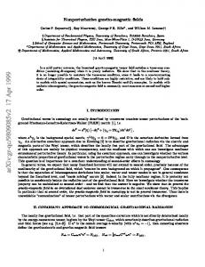
where y m is the magnetometer signal, m b is the local magnetic field expressed in the body frame. It includes the earth magnetic field and the local disturbances. The zero mean Gaussian white noise process is noted nm and characterized by a standard deviation σm . 3.2.2. Accelerometer The sensor axis is non-orthogonally calibrated using a dedicated platform for aligning each axis with the gravity field and applying a least squares based estimation. An Allan variance study [20] is applied to the accelerometer signal, which was acquired during a static phase, for inferring the noise characteristics. Figure 3 shows the Allan variance results plotted for one of the sensor axes.
Allan Variance (mg/sec/ √Hz)
Figure 3. Allan variance of the second component of the accelerometer. 10
0
10
-1
-2
10 -2 10
10
-1
10
0
10
1
10
2
10
3
10
4
Average time (sec)
Three main noise components are identified: an angular random walk, given by the −½ slope part, the bias instability, given by the 0 slope curve part and the beginning of a ½ slope curve at high average time. Consequently, the accelerometer signal is modelled by:
Sensors 2014, 14
22872
y a = fibb + ba + na
(12)
where the three dimensional sensor signal y a is composed by:
fibb the specific force of the body frame with respect to the inertial frame, expressed in the body frame; b a is the bias of the accelerometer and;
n a is a zero-mean Gaussian white noise with a standard deviation noted σ a . The bias b a is assumed to follow a Gauss-Markov model whose parameters are determined with the Allan variance study. The bias is mathematically expressed by:
b a = βb a + nba
(13)
where b a is the acceleration bias derivative, β is a constant and n ba is zero-mean Gaussian white noise with a standard deviation noted σba . The values of the accelerometer noise components are given in Table 1. Table 1. Accelerometer noise parameters.
Axis X Axis Y Axis Z
Velocity Random Walk Bias Instability Allan Deviation ( /√ ) 0.0650 0.1223 0.0717 0.0326 0.0639 0.0626
Correlated Noise Correlated Time (s) 0.1484 18.16 0.0373 48.05 0.0881 197.2
3.2.3. Gyroscope Similarly to the accelerometer signal, the gyroscope signal is studied over a long static phase and its Allan variance or spectral density is extracted. The angular rate is modeled by the following expression:
y g = ωbib + bω + nω
(14)
where:
y g , the three-dimension signal of the gyroscope, is composed with ωbib the angular rate of the body with respect to the inertial frame; bω is the gyroscope bias equivalent to an angular drift and;
nω is a zero-mean Gaussian white noise with a standard deviation noted σω . The gyroscope bias is modelled as a random walk:
b ω = nbω
(15)
where b ω is the gyroscope bias derivative and n bω is a zero-mean Gaussian white noise with standard deviation σ bω . All deviations are extracted from the Allan variance plotted in Figure 4.
Sensors 2014, 14
22873 Figure 4. Allan variance of gyroscope signal third component. -1
Allan Variance (deg/sec/ √Hz)
10
-2
10
-3
10 -2 10
-1
10
0
10
1
2
10 10 Average time (sec)
3
10
4
10
The angular rate ω bib can be decomposed in two parts Equation (16) by introducing the navigation frame, which is the plane locally tangent to the Earth. The angular rate of the body frame with respect to the navigation frame ωbnb is given by:
ωbib = ωbin + ωbnb
(16)
In the context of pedestrian navigation, the rotation of the navigation frame with respect to the inertial frame ω bin is rather small, as compared to the body dynamic expressed with ωbnb . So ω bin is assumed to be a residual part embedded in the gyroscope bias bω . The noise component values are given in Table 2. Table 2. Gyroscope noise parameters.
Axis X Axis Y Axis Z
Angular Random Walk Bias Instability Allan Deviation ( / /√ 0.00413 0.00117 0.00445 0.00121 0.00442 0.00105
Rate Random Walk ) 0.00158 0.00142 0.00157
3.3. Gyroscope Quaternion
3.3.1. Design of the Gyroscope Quaternion Model Instead of using directly the gyroscope model, the gyroscope signal is interpreted as a rotation between two successive epochs. A mathematical model of this rotation, named the quaternion gyroscope, is proposed and demonstrated. This new model results from the integration of Equation (10) using the navigation and body frames:
qbn (t + Ts ) = qbn (t ) ⊗ qω ( t ) where:
qω is the rotational quaternion between the two epochs t and t + Ts defined in (18); Ts is the sampling period and;
(17)
Sensors 2014, 14
22874
ωbnb is the angular rate of the body frame with respect to the navigation frame. The latter is assumed to be constant over the period t to t + Ts .
ωbnb cos T 2 s qω = f (ωbnb ) = ωbnb ωb Ts bnb sin ωnb 2
(18)
The gyroscope quaternion is constructed similarly to Equation (18), but instead of being composed of ωbnb , the quaternion gyroscope (noted q y g ) is composed of the gyroscope measurement (noted y g ):
qyg = f (y g )
(19)
The quaternion q y g is a rotational quaternion representing an approximation of qω , which is the rotation between two successive epochs. Following previous sensor error modelling, an Allan variance study of q y g , which has been created using all angular rates recorded during the static period, is conducted in order to assess the noise components of q y g . The same trend is observed for all four components. The low average time part corresponds to white noise. Figure 5 shows also a bias instability and a correlated or a rate random walk. Figure 5. Allan variance of the fourth dimension quaternion gyroscope. 10
Allan variance (rad/ √Hz)
10
10
10
10
10
-4
Quat.1
Quat.2
Quat.3
Quat.4
-6
-8
-10
-12
-14
10
-2
10
-1
10
0
10
1
10
2
10
3
10
4
Average time(sec)
Instead of modeling the gyroscope errors in the signal domain, it is performed in the quaternion set:
q y g = qω + bqω + nqω
(20)
where nqω is a zero-mean Gaussian white noise with standard deviation σ qω . The stochastic process chosen to model the gyroscope quaternion bias bqω is a random walk:
b qω = n bq
(21)
ω
where b qω is the gyroscope quaternion bias derivative and n bq is a zero-mean Gaussian white noise ω
with a standard deviation noted σ bq . ω
Sensors 2014, 14
22875
In order to a better understand the meaning of bqω , let us analyze the gyroscope quaternion q y g . This quaternion corresponds to a rotation that approximates the true rotation qω between two successive epochs. As a consequence, bqω appears to be the difference between both rotations. When it is small, it links the rotation qω to q y g by:
(
q y g = q ω I + q ω ⊗ b qω
(
)
(22)
)
where I + qω ⊗ b qω represents an infinitesimal rotation linking the qω to q y g . 3.3.2. Analysis of the Gyroscope Quaternion Bias MAGYQ attitude angles estimation filter is based on an Extended Kalman Filter (EKF) whose working hypothesis (H) is that only white noise components are not modeled in the state vector. Because the proposed angular rate modeling in the quaternion set is new, previous EKF working hypothesis is now demonstrated for the Model (20). Two approaches are followed for the demonstration. The first analysis studies the physical meaning of the quaternion bias term when the latter is small. The second approach exploits simulated angular rates transformed into the quaternion set for analyzing the distribution of the noise terms. Mathematical Derivation of the Gyroscope Quaternion Assuming that the angular rates and the gyroscope measurements are small (