2009 Microchip Technology Inc. DS00832B-page 1. AN832. OVERVIEW. This
application note explains methods for better tuning of resonant magnetic sensors
...
AN832 Magnetic Tuning of Resonant Sensors and Methods for Increasing Sensitivity Author:
Ruan Lourens Microchip Technology Inc.
OVERVIEW This application note explains methods for better tuning of resonant magnetic sensors typically used with Passive Keyless Entry (PKE) and RF Identification (RFID) devices. Also explained in this application note is a method to increase sensor sensitivity by means of magnetic concentration of the field.
Background A brief review of the differences between Passive Keyless Entry (PKE) and Remote Keyless Entry (RKE) is useful background information on this subject. We will use an example of PKE commonly found in the automotive industry. In this environment, PKE is bidirectional communication: magnetic from car to key fob and RF from key fob to car. An automatic challenge/ response dialog occurs when the user enters the relatively strong magnetic field surrounding the car. The magnetic field is generated in the base station (i.e., in the car) by setting up an oscillatory current at a low frequency of 125 kHz. This allows the user to unlock his/her car without pressing a button on a transmitter – very handy when carrying several items as when shopping. This method is termed “passive” keyless entry because the owner of the key fob does not have to press any buttons or take any action at all to initiate the communication between the key fob and the base station. The dialog happens automatically when the key fob enters the magnetic field of the base station. RKE is well-known in the automotive industry. This active method enables the user to unlock his/her car by pressing a button on the key fob. No magnetic field is used in this technique. Transmission is via unidirectional RF signals from the key fob to the vehicle.
Magnetic Sensor Considerations A typical magnetic low frequency (LF) sensor consists of a parallel inductor-capacitor circuit that is sensitive to an externally applied magnetic signal. This LC circuit is tuned to resonate at the source signal’s base frequency. The real-time voltage across the sensor represents the presence and strength of the surrounding magnetic field. By amplitude modulating the source’s magnetic field, it is possible to transfer data over short distances. This communication approach is successfully used with distances up to 1.8 meters, depending on transmission strengths and sensor sensitivity. Two key factors that greatly affect communication range are: 1. 2.
Sensor tuning. A properly tuned sensor’s relative sensitivity.
Magnetic tuning and magnetic concentration will be explained as influences on these two key factors. The accuracy of predicting a magnetic communication link’s behavior lies in correctly modeling the physical system. Herein lies a fundamental problem: magnetic circuits are generally not as well understood as electrical circuits. The experienced analog designer can design and analyze electronic circuits using accurate assumptions and simplifications, accurately reflecting a real system. The magnetic designer, on the other hand, quickly finds that magnetic circuit analysis simplification and modeling act merely as guidelines. One must revert back to Maxwell’s equations to account for physical manifestations observed when working with magnetic systems, but this is a tedious and complex process. A set of magnetic design guidelines and solutions will be explained in this document to accelerate the novice magnetic designer’s learning curve.
BASIC SENSOR CONCEPTS Certain fundamental concepts should be reviewed before moving to the magnetic solutions. This application note is not intended to be an in-depth study, but will merely highlight the basic concepts required. Most practical sensors consist of a small ferrite-based coil in parallel with a capacitor, with the values selected to resonate at the signal source’s frequency. This resonant tank circuit has various inherent losses such as: • Coil winding resistance • Core losses • Capacitor dissipation
© 2009 Microchip Technology Inc.
DS00832B-page 1
AN832 The combined effect of losses and load resistance can be reduced to a single resistor (see Figure 1) and the magnetic flux linkage with the coil can be represented as a current source at the carrier signal’s frequency.
FIGURE 1:
Vo is a maximum at the resonant frequency, calculated by Equation 2.
EQUATION 2:
Fo =
BASIC SENSOR CIRCUIT
+ iC
L
C
R
Vo
-
EQUATION 3:
Equation 1 expresses the absolute output value of the resonant tank circuit.
Im 2
The response is shown in Figure 2 for the following practical values: • • • •
C = 200 pF L = 8 mH R = 130 kΩ Im = 160 nA
The minimum sensitivity for an HCS473 is typically 20 mV, indicated in Figure 2. From the preceding values, one can see how sensitive the resonant tank is to resistive loading and how small the excitation current is. These considerations are more fully developed in the High-Impedance probe section of this application note.
DS00832B-page 2
1 = F2 − F1 2πRC
The quality factor, or “Q” of a resonant circuit is defined as the ratio of its resonant frequency to bandwidth, as shown in Equation 4.
EQUATION 1:
1 ⎛ 1 ⎞ + ⎜ ωC + ⎟ 2 R ⎝ ωL ⎠
2π LC
The bandwidth is the region between the -3 dB, or half power points, calculated by Equation 3.
BW =
Vo =
1
EQUATION 4:
Q=
Fo C =R L BW
The Q value is a good indication of the amount of coil losses. A low Q coil indicates that there are unnecessary losses associated with the sensor. A practical limit exists on the Q that is dictated by the tolerances of the components used. Production costs increase as tighter tolerance components are required to manufacture a properly tuned high-Q circuit. The higher the Q, the narrower the bandwidth, and the more susceptible the circuit becomes to the component tolerances shifting the resonant frequency outside the sensor’s most sensitive region.
© 2009 Microchip Technology Inc.
AN832 FIGURE 2:
FREQUENCY RESPONSE CURVE FOR RESONANT TANK CIRCUIT 35
F0
30
25
F2
V (mV rms)
F1 20
Vo -3dB 15
10
5
139600
138700
137800
136900
136000
135100
134200
133300
132400
131500
130600
129700
128800
127900
127000
126100
125200
124300
123400
122500
121600
120700
119800
118900
118000
117100
116200
115300
114400
113500
112600
111700
110800
F
0
F (Hz)
MANUFACTURING TOLERANCES A good rule of thumb is to stay within the -3 dB limits, giving component tolerances by Equation 5.
EQUATION 5:
Q≤
Tcap
1 + Tind
TCAP and TIND are the individual manufacturing tolerances for capacitance and inductance. For 2% parts, a Q of 20 works very well. Lower tolerance components may be used at the expense of sensitivity, and thus yielding a lower range. The corresponding final design must accommodate a wider bandwidth and will, therefore, have a lower response. On the other hand, to design a ferrite-based coil with reasonable dimensions and a Q of much higher than 25 soon becomes either too expensive or too impractical to implement.
ELECTROMAGNETISM BASICS It is important to note the difference between a magnetic field/electric field versus an electromagnetic wave. A magnetic field is a result of electrical charge in motion, or a magnetic dipole. One only gets magnetic dipoles and not monopoles, as is the case for electrical particles. A magnetic field can be represented by field lines that form continuous loops that never cross each other.
© 2009 Microchip Technology Inc.
Electric fields, on the other hand, are the result of a distributed electrical charge. What both magnetic and electric fields share in common is that the field strength of both fields attenuates at a rate of 1/R3 when the source geometry is assumed to be a point source. What this means is that the field intensity at a distance 2X away from the source is 1/8th of the field intensity measured at a distance X from the source. However, an electromagnetic wave reacts quite differently than the magnetic or electric field. Assuming the same point source, the electromagnetic wave propagates with a decay rate of 1/R. Thus, at a distance of 2X from the point source, the field intensity is only 1/2 compared to that which is measured at a distance of X from the source. This means that a magnetic field decays much more rapidly than an electromagnetic wave. For most RFID and PKE applications, a magnetic field is generated in the base station by setting up an oscillatory current in a series RLC network at a typical frequency of 125 kHz. The current passing through the inductor creates a surrounding magnetic field according to Ampere’s Law. Using Equation 6, one can calculate the magnetic field strength at a point P from the radiating coil, as shown in Figure 3.
EQUATION 6:
|B| p =
(
μoINa2 2
2 a +r
)
2 32
≈
μoINa2 2r 3
[Weber / m 2 ] r >> a
DS00832B-page 3
AN832 FIGURE 3:
CALCULATING MAGNETIC FIELD STRENGTH
If the signal wavelength (magnetic or electric) approaches the dimension of the antenna, the magnetic electric reinforcement gets strong enough to allow for electromagnetic wave propagation. Thus, for an antenna that is very small compared to the signal wavelength, one does not have an efficient propagating wave decaying at 1/r; instead, one has an attenuating field that falls off at 1/r.3 Higher frequency antenna dimensions are thus much more practical and a true propagating wave is easily realizable.
X
a r
P
Y
Note:
Z
Note:
For r2 > a2, the field strength falls off with 1/r3.
A component of the total energy is in the form of an electromagnetic wave, but that is negligible compared to the magnetic energy with a 125 kHz magnetic antenna.
There are practical reasons why a magnetic field is chosen for base station to key fob communications, as shown in Table 1.
The field strength is proportional to: • the number of turns (N) • the current (I) • the area of the loop (a2) The antenna coil also generates an electric field due to the induced voltage over the coil, but it is not as dominant as the magnetic effect. The electric field also falls off at a 1/r3 rate, as stated, and the electromagnetic waves decay at a 1/r rate. The question is, then, what is the link between magnetic/electric fields and electromagnetic waves? To find the answers, we need to consider some properties of both magnetic and electric fields. The first is that a time-varying electric field induces a magnetic field and, conversely, that a time-varying magnetic field induces an electric field. These are special cases of Amperes and Faraday’s laws, respectively. Therefore, a time-varying field of either kind induces and reinforces a field of the other kind. One thus gets a slightly stronger field when compared to Equation 6. The effect, however, is negligible if the antenna dimension is small relative to the wavelength of the exciting signal. The wavelength of a signal can be calculated from Equation 7, and at 125 kHz is a long length of 2.4 km.
EQUATION 7:
λ=
c (m ) c = 3x10⁸ m/s f
An antenna approaching this dimension is impractical, but at 500 MHz the wavelength is only 60 cm.
TABLE 1:
Practical Reason
Justification
Controlled Range
Magnetic fields fall off at a 1/r3 rate compared to electromagnetic waves that attenuate at a 1/r rate. This is required when communications should only happen in close proximity (i.e., busy parking lot with many cars).
Flexibility of carrier
Good field penetration compared to RF and does not require line-of-sight, as for IR.
Cost
LF components are relatively cheap due to lower speed requirements.
Low-Current Consumption
It is possible to build a LF receiver with very low biasing currents at the key fob side. An HCS473 typically consumes less than 6 μA.
However, it is practical to use true RF waves for communicating from the key fob back to the base station for the following reasons: 1.
2.
3.
DS00832B-page 4
REASONS FOR CHOOSING MAGNETIC TUNING SOLUTION
A key fob also needs RKE functions, and it would be useless if the RKE range was limited to 2 meters. The RF stage in the key fob transmits only infrequently and one can tolerate a few milliamps of power drain during transmission. A magnetic antenna draws too much current for a key fob, and the range is limited.
© 2009 Microchip Technology Inc.
AN832 WAYS OF IMPROVING MAGNETIC SENSOR SENSITIVITY There are three ways that are known to improve the sensitivity of magnetic sensors: 1.
2.
3.
Magnetic Tuning – The more precise the tuning of the sensor, the more sensitive it becomes to changes in the surrounding magnetic field. Magnetic Field Concentration – The more lines of magnetic force that can be focused through a sensor, the more sensitive it becomes and the greater the range. Limiting of Interference – The more the interference from surrounding components and circuits is reduced, the more efficient and thus more sensitive the sensors become.
Tuning Magnetic circuits PROBLEMS WITH CONVENTIONAL ELECTRICAL TUNING METHODS When using transponders and other magnetic sensor circuits, it is important to have the transmitter and receiver resonant at the same frequency. The current approach used is to electrically tune the sensor circuit to resonate at the required frequency. This method typically applies a time-varying source to the circuit and measures the output response using a bridge analyzer as shown in Figure 4.
FIGURE 4:
SOURCE
CONVENTIONAL ELECTRICAL TUNING METHOD
METER OR BRIDGE ANALYZER
L
C
R
The sensor is excited with some electrical signal to either measure its frequency response, or its inductance, yet it is used as a magnetic field sensor. The magnetic environment around the sensor is, to a large extent, ignored when driving the coil electrically. However, the environment has an enormous influence on the magnetic field which the sensor is supposed to measure. Objects such as batteries and RF circuits distort the magnetic field and absorb magnetic energy when placed in the sensor’s magnetic field path. To complicate matters further, the effects are nonlinear. The effects are nonlinear because inductance changes as a function of flux density, thus the resonant frequency is different for strong and weak signal conditions.
THE MAGNETIC TUNING SOLUTION To obtain optimal performance from a magnetic sensor, one needs an easy solution to accurately tune a magnetic resonant circuit. The solution is to excite the sensor in a time-varying magnetic field instead of driving the sensor electrically. The process requires only basic lab equipment and can be performed very quickly. A properly tuned sensor is one in which the sensor’s resonant frequency coincides with the frequency of the exciting magnetic field. Through proper tuning, the same magnetic field results in a much larger voltage across the sensor. The basic test setup for performing magnetic tuning of resonant sensors shown in Figure 5 consists of: • • • •
A signal source Two multi-meters or oscilloscopes An air coil A custom, active, high-impedance probe
FIGURE 5:
BASIC TEST SETUP Air Coil
Signal Generator What most designers currently do to ‘tune’ the sensor to resonate at a desired frequency is to very accurately measure the sensor coil’s inductance and calculate the required capacitance (taking parasitic capacitance into account). Another ‘electric’ approach is to connect the sensor to a bridge analyzer and characterize its electrical frequency response. The designer soon realizes that both approaches fail to yield repeatable, optimal solutions. There are various reasons why an ‘electric’ solution fails, but the most dominating factors can be explained briefly.
© 2009 Microchip Technology Inc.
Multimeter A
Test Coil
High Impedance Probe
Multimeter B
DS00832B-page 5
AN832 Driving a low inductance air coil directly from a signal source generates a weak magnetic field, and it is with weak field conditions that tuning is critical. The test coil is placed at such a distance from the exciting air coil as to simulate the typical trigger voltage of 15 mVRMS. The response is measured via a high-impedance probe specifically developed for this application. The probe is designed to be used either as a buffer or as a true value RMS-to-DC converter. When using a multimeter, or an oscilloscope capable of measuring at 125 kHz, one can use the probe purely as a buffer. In the ‘true value RMS-to-DC converter’ mode one can measure the response with a normal handheld DC multimeter. The latter is not as accurate, but is accurate enough for the application. The second multimeter (see Multimeter A in Figure 5) is used to ensure that the coil response is flat around the resonant frequency, since the normal 50 ohm output of the signal generator is easily loaded. The magnetic tuning approach consistently gives better results than electric tuning. In one instance, magnetic tuning improved an existing design’s sensitivity by 800%. In that instance, it was shown that the resonant frequency at low field strengths was 139 kHz instead of the desired 125 kHz, because it had been tuned electrically. A high-impedance LF probe is at the heart of tuning magnetic sensors accurately; a normal high-impedance oscilloscope probe does not work for tuning magnetic sensors due to capacitive loading of the delicate circuitry. The typically designed sensors have a resonant capacitance below 200 pF and an oscilloscope probe is at least 10 pF. To make things worse, it uses a co-axial cable to connect back to the meter (which adds more loading to the circuit).
THE MAGNETIC TUNING PROCESS The magnetic tuning process is normally done in a couple of stages to arrive at the optimal values for a specific magnetic design. In this process it is important that all the factors which may influence a design from a magnetic perspective be included. The most basic factors to consider when tuning are: • Make sure to stay within the component tolerance guidelines. • Tune the device as a system. Changing battery location or enclosures has a big influence on the sensors magnetic environment. Make sure that as many as possible of the final system conditions are met. • Tune with the device removed, because the probe simulates the influence of the device and having both present at the same time will cause the final sensor to resonate at a higher than desired frequency. • Tuning should be done in weak field conditions to simulate the field far away from the base station. These guidelines will ensure better production yields such that the units can be manufactured to give repeatable results without having to tune each specific unit. Figure 6 shows a flowchart of the procedure for performing the tuning of the magnetic sensors.
Experiments with different test setups have shown greatly varying results due to measurement equipment loading the tuned circuit. One approach used a highimpedance FET voltage follower, but even it gave inconsistent readings due to asymmetrical changes in the input capacitance. Another requirement for a good measurement probe is to simulate the end-user device environment impedance and capacitance. For the HCS473, the input impedance is very high at 1012Ω and the input capacitance is about 6 pF. The eventual solution that gave very good results was to use a high quality instrumentation amplifier with similar input characteristics. A total LF test probe design with an RMSto-DC converter schematic is shown in Appendix A.
DS00832B-page 6
© 2009 Microchip Technology Inc.
AN832 FIGURE 6:
MAGNETIC TUNING PROCESS FLOWCHART Start
1. Measure the inductance of the sensor coil without the capacitor present. 2. Using the measured inductance value, calculate the required capacitor using Equation 2. Subtract the probe capacitance (5 pF) from the calculated capacitance size and choose a capacitor to closely match this value. 3. With this known capacitance (C1) in place, start the tuning process by placing the sensor in the weak field. 4. Connect the test coil to the probe input with short wires and set the probe gain to x100, U1 to x10, and U2 to x10. 5. Place the coil under test along its sensitive axis to give an output of roughly 15 mVRMS. 6. Perform a sweep of the frequency of the field to find the sensor’s resonant frequency. 7. Once in this rough resonant frequency region, set the sweep sensitivity to 10’s of Hz and find a more accurate center frequency. 8. Log the center frequency and the eventual output voltage at resonance as F0 and VMAX. 9. Calculate the -3 dB voltage. Find the two cutoff frequencies F1 and F2 (see Figure 2). 10. With F0, F1 and F2 known, calculate the Q (see Equation 4). 11. Calculate the magnetic inductance with C1, F0 and probe capacitance (CP), replacing C with C1 + CP into Equation 2:
1 F 0 = ---------------------------------------2π L ( C1 + C P )
ADDITIONAL DETAILS OF THE TUNING PROCESS SHOWN IN FIGURE 6 • In Step 2 it is important to measure the capacitor values very carefully, in a repeatable manner, since this will determine final accuracy. Do not use flexible wires on the capacitance meter. Use a fixed test setup only. • In Step 3 the field is set up as in Figure 5 by connecting an air coil (100 H to 1 mH) to a signal generator at 125 kHz and output amplitude of 50 mV to 200 mV. A low output voltage is chosen to reduce loading effects on the signal generator’s 50 ohm output impedance. • In Step 5 with the total probe gain of x100, this translates to 1.5 VDC to keep within the requirement to have the output at 0.5 VDC to 5 VDC when using the RMS-to-DC converter stage. • In Step 6 a good guideline is to sweep the frequency in 100 Hz steps until the rough resonant frequency is located. • In Step 8 note F0 is the center of the response curve shown in Figure 2. • In Step 9 calculate the -3 dB voltage by Vm/ sqrt(2) and then find the two cutoff frequencies F1 and F2 where this amplitude coincides (see Figure 2). The cutoff frequencies can be determined more accurately than F0 that is at a flat crest, and the average of F1 and F2 is a more accurate value for F0. • When replacing capacitors, make sure to use the manufacturer-recommended solder flux and clean off the flux before testing. Incorrect flux and improper cleaning will cause inconsistency and low Q. Another practical tip on capacitors is to use good quality NPO (Panasonic) or equivalent capacitors with good temperature stability and low losses. Note:
Is F0 = required frequency?
Yes
Done
This process must be repeated only once for new designs. Once the tuning process is completed, the values can be used in production as long as the tolerances of the production units stay within specifications.
No With the newly-calculated inductance, one can calculate the second iteration capacitance C2 required to get F0 to 125 kHz. One can repeat this process across a range of samples to get to the best values to use in final production.
© 2009 Microchip Technology Inc.
DS00832B-page 7
AN832 Magnetic Field Concentration
FIGURE 7:
FIELD PATH FOR NORMAL FERRITEBASED COIL
FIGURE 8:
FIELD PATH WITH TWO PIECES OF MAGNETIC MATERIAL ADDED
To increase the range of a PKE transponder one has limited options, and the three major approaches are: • Increase the device sensitivity; to achieve higher receiver sensitivity one normally needs to increase the bias current of the receiver in Standby mode. The transponders are battery operated and clients normally require a long battery life (5-10 μA). • Increase the field strength; there are, however, regulatory limits to the field strength allowed when transmitting at 125 kHz, and these vary from country to country. • Increase magnetic receiver sensitivity; this is an often overlooked area and here one can achieve substantial gains at a relatively low cost. The basic concept behind the patent is to focus a larger-than-normal window of flux through the coil. This can be achieved by either: • Adding a flux concentration device external to an existing coil • Incorporating a flux concentration device into the coil Figure 7 shows the field path through a normal ferritebased coil when placed in an externally applied magnetic field. The result of adding two pieces of magnetic material (typically ferrite) external to the coil is shown in Figure 8. The results clearly show that it concentrates more flux through the sensor. There are limits as to how far this approach can be taken and the limiting factors are: • Inductance; the inductance of a coil increases making the resonant capacitor small. A good guideline is to try and keep the final inductance below 13 mH and above 8 mH. One should use closer tolerances as is suggested by Equation 5. • Hysteresis losses; a point is reached where adding more magnetic material increases losses more than it increases sensitivity. • Size and practicality.
DS00832B-page 8
© 2009 Microchip Technology Inc.
AN832 Limiting Magnetic Interference The following are some practical guidelines to follow that will limit interference when placing multiple sensors close to each other to cover multiple axes: • Do not place ferrite-cored sensors too close to each other. Coils placed too close to each other form a weakly-coupled transformer. The result is that one coil can cause resonance in another coil that is not in the strong field direction, and the available field energy gets shared with a resulting decrease in sensitivity. A good test for this effect is to see if a specific coil’s resonant frequency changes when short-circuiting the other coil. If so, increase the distance between coils. The effect can also be observed as double resonance and a change in Q. The process is known as ‘mutually coupled resonant circuits’ and a lot of information is available on the subject. For PKE, avoid it by increasing the inter-coil distances. • For PKE applications, one axis is normally in the form of an air coil, which can also have an influence on the ferrite-based coils. Make sure that it does not cross another coil but instead, either totally surrounds it, (as shown in Figure 9) or is completely removed from the ferrite coils (as shown in Figure 10). • A good rule of thumb for small ferrite coils is to maintain a separation distance between coils of at least 7 mm at the closest point. Figure 11 shows the optimum placement of ferrite coils for best results.
FIGURE 9:
AIR COIL SURROUNDING FERRITE COILS
FIGURE 10:
AIR COIL REMOVED FROM FERRITE COILS
Air Coil
Ferrite Coils
FIGURE 11:
OPTIMUM PLACEMENT OF FERRITE COILS
X
Y
Ferrite Coils
NOTE: For best results choose X ≅ Y
Air Coil
Ferrite Coils
© 2009 Microchip Technology Inc.
DS00832B-page 9
AN832 A CLOSER LOOK AT THE HCS473 The HCS473 is a 3-axis PKE transponder. The HCS473 combines the patented KEELOQ® code hopping technology and bidirectional transponder challenge-and-response security into a single chip solution for logical and physical access control. The three input transponder interface allows the combination of three orthogonal transponder antennas to eliminate the directionality traditionally associated with transponder systems. When the HCS473 is used as a code hopping encoder device, it is best suited for use in keyless entry systems such as vehicles and home garage door openers. It is meant to be a cost-effective, yet secure solution to such systems. The HCS473 can also be used as a secure bidirectional transponder for verification of a token. This makes the HCS473 ideal for secure access control and identification applications. A single HCS473 can be used as an encoder for Remote Keyless Entry (RKE) and a transponder for immobilization and Passive Keyless Entry (PKE) in the same circuit. This dramatically reduces the cost of hybrid transmitter/ transponder circuits. Figure 12 shows a typical model using an HCS473 when three resonant sensors are connected to the device. These are the three sensors and their associated tank capacitors shown in Figure 6, The Tuning Process Flowchart.
DS00832B-page 10
© 2009 Microchip Technology Inc.
AN832 FIGURE 12:
RESONANT SENSOR CONNECTIONS
Internal to HCS473
R1 Interpad Cap C5 4 pF
X
losses
130 kOhm C1
pad cap C9 6 pF
Interpad Cap
Internal to HCS473
External to HCS473
200 pF L1
R2
Serial Resistance
Comparator
500 ohm Y
I1
8 mH Air Coil C6 4 pF V1
X
Comparator +
Noise Source 125 kHz Signal Source R3
Y
Z
160 kOhm C2
pad cap C10 6 pF
135 pF L3
R4 100 ohm
Common
Comparator
200 KΩ
X
12 mH Ferrite Coil I3
C4/CCOMMON 1.5 NF
6 pF
±
C7 4 pF Interpad Cap
0.6 V
125 kHz Signal Source R5
Z
pad cap C11 6 pF
160 kOhm C3 135 pF L2
C8 4 pF Interpad Cap
R6 100 ohm
12 mH Ferrite Coil
I2
125 kHz Signal Source
The HCS473 is a microcontroller with an analog frontend for receiving PKE signals. The designer should be aware that the microcontroller itself can be a substantial noise source. The air coil is also a good antenna for picking up noise, and can initiate oscillation. A common pin exists for the three devices and each coil has its own input (three axes are necessary to cover 3D space). C4 is added for stability. If C4 is too small, the system becomes unstable. The value of CCOMMON will vary from design to design. The system designer needs to ensure stability under all conditions. A good start is to perform a theoretical stability analysis on the complete sensor system. One finds that the system can easily become serial resonant if C4/CCOMMON is too small.
An example of series resonance is when L1 and CCOMMON form a resonant tank circuit at a resonant frequency given by Equation 8:
EQUATION 8: 1 F 0 = -------------------------------------------------2π L1 × CCOMMON For practical verification and debugging, the HCS473 offers a raw data test. In this test, the received data is output directly and the designer should ensure that this signal is stable, without notches or glitches. Instability is more likely to occur at maximum input voltage and cold temperatures. Make sure that the CCOMMON pin is stable. The mode of instability is serial resonance with sensor coils, as stated earlier. The analog front-end circuits and microcontroller circuits of the HCS473 have separate power supplies.The designer should ensure good grounding and decoupling of all power supplies.
© 2009 Microchip Technology Inc.
DS00832B-page 11
AN832 APPENDIX A:
LF TEST PROBE
FIGURE A-1:
RMS-TO-DC SENSITIVITY PROBE SCHEMATIC
TP1
TP2 +15V
+
C1 4.7μF
TP3
+15V
+
RP1 1 2K 3
R4 9.1K
C3 0.1μF
C2 4.7μF
TP4
2
U1 1 13 JP1 *Note 1 12 x10 x100
JP2
GAIN ADJUSTMENT
C7 10pF
-15V
TP5
16 11 3 2
-
INA110KP
8 4
+VS
x10
IN ADJ
x100 x200 x500 Rg -VS
+
+15V
OUT ADJ
TP6
5 IN ADJ
10
R2 10K 1%
x1
SENS
OUT OUT REF ADJ 6 15
9
R1 4.7M
JP4*Note 2 R3 1K 1%
14
R7 24K 1%
SIGNAL
C6 0.1μF
7
-15V TP8 TP9
-15V U3
+15V C13 2200pF RP2 50K
ZERO OFFSET ADJUSTMENT
R5 2M 2
3
+ C14 3.3μF
C8 6 OUT OFFSET 3 + TRIM 10nF 5 V1 TP7 4
2 -
x10
BUFFER 1 BUF IN + 2 NC ANA 3 COM
5 CS
-15V
6 DEN IN R6 62Ω
BUF OUT 14 ABSOLUTE VALUE
7 dB
25k
12 11
+Vs
10
-Vs SQUARER/DIVIDER 25k
-
+
AD637JQ
C9 0.1μF +15V -15V C10 0.1μF
RMS OUT 9
+ FILTER CAV 8
+15V
RMS_OUT
SIG IN 13 NC
OUT BIAS 4 OFF SECTION
1
JP6
LM602BP
V+
JP3 C4 0.1μF
C5 0.1μF
U2 7
C11 680pF
+ C12 1.0μF
JP5
Note 1: No jumper is installed in JP1 to achieve unity gain. 2: A jumper selection must be made for JP4. 3: Unless otherwise specified: Resistance values are in ohms. Resistors are 5: tolerance. Capacitance values are in μF. 4: Device names and numbers shown here are for reference only and may differ from the actual number.
DS00832B-page 12
© 2009 Microchip Technology Inc.
AN832 Circuit Description U1 is an instrumentation amplifier from analog devices, and the coil under measurement is connected to JP2. As previously mentioned, the user can either use U1 as a buffer and read its output at TP6, or use the rest of the circuit as an RMS-to-DC converter. Zero offset is adjusted with RP2 and gain is set by RP1. The RMSto-DC converter must be used to give an output of between 0.5 and 5 VDC. This is accomplished by changing the gain in two stages with JP1 and JP4. JP1 can give unity gain, (no jumper present), x10 or x100. The device can handle higher gains, but linearity degrades proportionally. The second gain stage is via U2 and its gain is set to either unity or x10 gain via jumper 4. The integration period for U3 is 280 μs with JP5 and JP6 open, and about 0.5 seconds with the jumpers in place. If the probe and coil under test have isolated ground paths (as is normally the case) make sure that the jumper JP3 is in.
© 2009 Microchip Technology Inc.
DS00832B-page 13
AN832 TABLE 2:
LF TEST PROBE BILL OF MATERIALS
Qty Ref. #
Description
Value
Manufacturer
Mfr. Part Number
6
C3 C4 C5 C6 C9 C10
Cap, 0.1 μF, Ceramic, X7R, 10%, 50V
0.1 μF
BC Components K104K15X7RF5TI2
1
C8
Cap, 10 nF, Ceramic, X7R, 10%, 50V
10 nF
BC Components K103K15X7RF5TI2
1
C11
Cap, 680 pF, Ceramic, C0G, 5%, 50V
680 pF
BC Components K681J15C0GF5TL2
1
C13
Cap, 2200 pF, Ceramic, C0G, 5%, 50V
2200 pF
BC Components K222J15C0GF5TL2 BC Components K100J15C0GF5TL2
1
C7
Cap, 10 pF, Ceramic, C0G, 5%, 50V
10 pF
1
C12
Cap, 1.0 μF, Radial, Aluminum, Electrolytic, 50V
1.0 μF
1
C14
Cap, 3.3 μF, Radial, Aluminum, Electrolytic, 50V
3.3 μF
Panasonic
ECE-A1HKG3R3
2
C1 C2
Cap, 4.7 mF, Radial, Aluminum, Electrolytic, 50V
4.7 μF
Panasonic
ECE-A1HKG4R7
1
U3
IC, Wide-Band RMA-to-DC Converter, 14-CDIP
AD637JQ
1
U1
IC, FET-Input Instrumentation Amp, 16-DIP
INA110KP
Burr-Brown
INA110KP
1
U2
IC, High-Speed Precision Op Amp, 8-DIP
OPA602BP
Burr-Brown
OPA602BP
4
JP2 JP3 JP5 JP6
Con, Header Connector, 1X2, .100” Pitch
1x2
Samtec
TSW-102-07-S-S
2
JP1 JP4
Con, Header Connector, 1X3, .100” Pitch
1x3
Samtec
TSW-103-07-S-S
1
RP1
Pot, 2.0 kOhm, 1/4 Square, Cermet, Multi-turn
2.0K
Bourns
3266W-1-202
1
RP2
50K
Bourns
3266W-1-503
1
R3
Res, 1.00 kOhm, 1/4 W, 1%, Metal Film
1.00K
Yageo
MFR-25FBF-1K00
1
R5
Res, 2.0 mOhm, 1/4 W, 5%, Carbon Film
2.0M
Yageo
CFR-25JB-2M00
1
R1
Res, 4.7 mOhm, 1/4 W, 5%, Carbon Film
4.7M
Yageo
CFR-25JB-4M7
Pot, 50 kOhm, 1/4 Square, Cermet, Multi-turn
Panasonic
ECE-A1HKG010
Analog Devices AD637JQ
1
R4
Res, 9.1 kOhm
9.1K
Yageo
CFR-25JB-9K1
1
R2
Res, 10.0 kOhm, 1/4 W, 1%, Metal Film
10.0K
Yageo
MFR-25FBF-10K0
1
R7
Res, 24.3 kOhm, 1/4 W, 1%, Metal Film
24.3K
Yageo
MFR-25FBF-24K3
1
R6
Res, 62 Ohm, 1/4 W, 5%, Carbon Film
62
Yageo
CFR-25JB-62R
1
TP1
Tsp, Test Point, Multi-Purpose, Red
Red
Keystone
5010
2
TP3 TP9
Tsp, Test Point, Multi-Purpose, Black
Black
Keystone
5011
5
TP4 TP5 TP6 TP7 TP8
Tsp, Test Point, Multi-Purpose, White
White
Keystone
5012
1
TP2
Tsp, Test Point, Multi-Purpose, Yellow
Yellow
Keystone
5014
1
SU1
Soc, 16-Pin Socket, Gold, Machine Pins
16-Pin
Mill-Max
110-93-316-41-001
1
SU2
Soc, 8-Pin Socket, Gold, Machine Pins
8-Pin
Mill-Max
110-93-308-41-001
1
SU3
Soc, 14-Pin Socket, Gold, Machine Pins
14-Pin
Mill-Max
110-93-314-41-001
DS00832B-page 14
© 2009 Microchip Technology Inc.
AN832 FIGURE A-2:
LF TEST PROBE PRINTED CIRCUIT BOARD, BOTTOM VIEW
FIGURE A-3:
LF TEST PROBE PRINTED CIRCUIT BOARD, TOP VIEW
Note:
The PCB and schematics are available on the Microchip web site at www.microchip.com or by contacting Microchip.
© 2009 Microchip Technology Inc.
DS00832B-page 15
AN832 NOTES:
DS00832B-page 16
© 2009 Microchip Technology Inc.
Note the following details of the code protection feature on Microchip devices: •
Microchip products meet the specification contained in their particular Microchip Data Sheet.
•
Microchip believes that its family of products is one of the most secure families of its kind on the market today, when used in the intended manner and under normal conditions.
•
There are dishonest and possibly illegal methods used to breach the code protection feature. All of these methods, to our knowledge, require using the Microchip products in a manner outside the operating specifications contained in Microchip’s Data Sheets. Most likely, the person doing so is engaged in theft of intellectual property.
•
Microchip is willing to work with the customer who is concerned about the integrity of their code.
•
Neither Microchip nor any other semiconductor manufacturer can guarantee the security of their code. Code protection does not mean that we are guaranteeing the product as “unbreakable.”
Code protection is constantly evolving. We at Microchip are committed to continuously improving the code protection features of our products. Attempts to break Microchip’s code protection feature may be a violation of the Digital Millennium Copyright Act. If such acts allow unauthorized access to your software or other copyrighted work, you may have a right to sue for relief under that Act.
Information contained in this publication regarding device applications and the like is provided only for your convenience and may be superseded by updates. It is your responsibility to ensure that your application meets with your specifications. MICROCHIP MAKES NO REPRESENTATIONS OR WARRANTIES OF ANY KIND WHETHER EXPRESS OR IMPLIED, WRITTEN OR ORAL, STATUTORY OR OTHERWISE, RELATED TO THE INFORMATION, INCLUDING BUT NOT LIMITED TO ITS CONDITION, QUALITY, PERFORMANCE, MERCHANTABILITY OR FITNESS FOR PURPOSE. Microchip disclaims all liability arising from this information and its use. Use of Microchip devices in life support and/or safety applications is entirely at the buyer’s risk, and the buyer agrees to defend, indemnify and hold harmless Microchip from any and all damages, claims, suits, or expenses resulting from such use. No licenses are conveyed, implicitly or otherwise, under any Microchip intellectual property rights.
Trademarks The Microchip name and logo, the Microchip logo, Accuron, dsPIC, KEELOQ, KEELOQ logo, MPLAB, PIC, PICmicro, PICSTART, rfPIC, SmartShunt and UNI/O are registered trademarks of Microchip Technology Incorporated in the U.S.A. and other countries. FilterLab, Linear Active Thermistor, MXDEV, MXLAB, SEEVAL, SmartSensor and The Embedded Control Solutions Company are registered trademarks of Microchip Technology Incorporated in the U.S.A. Analog-for-the-Digital Age, Application Maestro, CodeGuard, dsPICDEM, dsPICDEM.net, dsPICworks, dsSPEAK, ECAN, ECONOMONITOR, FanSense, In-Circuit Serial Programming, ICSP, ICEPIC, Mindi, MiWi, MPASM, MPLAB Certified logo, MPLIB, MPLINK, mTouch, PICkit, PICDEM, PICDEM.net, PICtail, PIC32 logo, PowerCal, PowerInfo, PowerMate, PowerTool, REAL ICE, rfLAB, Select Mode, Total Endurance, WiperLock and ZENA are trademarks of Microchip Technology Incorporated in the U.S.A. and other countries. SQTP is a service mark of Microchip Technology Incorporated in the U.S.A. All other trademarks mentioned herein are property of their respective companies. © 2009, Microchip Technology Incorporated, Printed in the U.S.A., All Rights Reserved. Printed on recycled paper.
Microchip received ISO/TS-16949:2002 certification for its worldwide headquarters, design and wafer fabrication facilities in Chandler and Tempe, Arizona; Gresham, Oregon and design centers in California and India. The Company’s quality system processes and procedures are for its PIC® MCUs and dsPIC® DSCs, KEELOQ® code hopping devices, Serial EEPROMs, microperipherals, nonvolatile memory and analog products. In addition, Microchip’s quality system for the design and manufacture of development systems is ISO 9001:2000 certified.
© 2009 Microchip Technology Inc.
DS00832B-page 17
WORLDWIDE SALES AND SERVICE AMERICAS
ASIA/PACIFIC
ASIA/PACIFIC
EUROPE
Corporate Office 2355 West Chandler Blvd. Chandler, AZ 85224-6199 Tel: 480-792-7200 Fax: 480-792-7277 Technical Support: http://support.microchip.com Web Address: www.microchip.com
Asia Pacific Office Suites 3707-14, 37th Floor Tower 6, The Gateway Harbour City, Kowloon Hong Kong Tel: 852-2401-1200 Fax: 852-2401-3431
India - Bangalore Tel: 91-80-4182-8400 Fax: 91-80-4182-8422 India - New Delhi Tel: 91-11-4160-8631 Fax: 91-11-4160-8632
Austria - Wels Tel: 43-7242-2244-39 Fax: 43-7242-2244-393 Denmark - Copenhagen Tel: 45-4450-2828 Fax: 45-4485-2829
India - Pune Tel: 91-20-2566-1512 Fax: 91-20-2566-1513
France - Paris Tel: 33-1-69-53-63-20 Fax: 33-1-69-30-90-79
Japan - Yokohama Tel: 81-45-471- 6166 Fax: 81-45-471-6122
Germany - Munich Tel: 49-89-627-144-0 Fax: 49-89-627-144-44
Atlanta Duluth, GA Tel: 678-957-9614 Fax: 678-957-1455 Boston Westborough, MA Tel: 774-760-0087 Fax: 774-760-0088 Chicago Itasca, IL Tel: 630-285-0071 Fax: 630-285-0075 Dallas Addison, TX Tel: 972-818-7423 Fax: 972-818-2924 Detroit Farmington Hills, MI Tel: 248-538-2250 Fax: 248-538-2260 Kokomo Kokomo, IN Tel: 765-864-8360 Fax: 765-864-8387 Los Angeles Mission Viejo, CA Tel: 949-462-9523 Fax: 949-462-9608 Santa Clara Santa Clara, CA Tel: 408-961-6444 Fax: 408-961-6445 Toronto Mississauga, Ontario, Canada Tel: 905-673-0699 Fax: 905-673-6509
Australia - Sydney Tel: 61-2-9868-6733 Fax: 61-2-9868-6755 China - Beijing Tel: 86-10-8528-2100 Fax: 86-10-8528-2104 China - Chengdu Tel: 86-28-8665-5511 Fax: 86-28-8665-7889
Korea - Daegu Tel: 82-53-744-4301 Fax: 82-53-744-4302
China - Hong Kong SAR Tel: 852-2401-1200 Fax: 852-2401-3431
Korea - Seoul Tel: 82-2-554-7200 Fax: 82-2-558-5932 or 82-2-558-5934
China - Nanjing Tel: 86-25-8473-2460 Fax: 86-25-8473-2470
Malaysia - Kuala Lumpur Tel: 60-3-6201-9857 Fax: 60-3-6201-9859
China - Qingdao Tel: 86-532-8502-7355 Fax: 86-532-8502-7205
Malaysia - Penang Tel: 60-4-227-8870 Fax: 60-4-227-4068
China - Shanghai Tel: 86-21-5407-5533 Fax: 86-21-5407-5066
Philippines - Manila Tel: 63-2-634-9065 Fax: 63-2-634-9069
China - Shenyang Tel: 86-24-2334-2829 Fax: 86-24-2334-2393
Singapore Tel: 65-6334-8870 Fax: 65-6334-8850
China - Shenzhen Tel: 86-755-8203-2660 Fax: 86-755-8203-1760
Taiwan - Hsin Chu Tel: 886-3-572-9526 Fax: 886-3-572-6459
China - Wuhan Tel: 86-27-5980-5300 Fax: 86-27-5980-5118
Taiwan - Kaohsiung Tel: 886-7-536-4818 Fax: 886-7-536-4803
China - Xiamen Tel: 86-592-2388138 Fax: 86-592-2388130
Taiwan - Taipei Tel: 886-2-2500-6610 Fax: 886-2-2508-0102
China - Xian Tel: 86-29-8833-7252 Fax: 86-29-8833-7256
Thailand - Bangkok Tel: 66-2-694-1351 Fax: 66-2-694-1350
Italy - Milan Tel: 39-0331-742611 Fax: 39-0331-466781 Netherlands - Drunen Tel: 31-416-690399 Fax: 31-416-690340 Spain - Madrid Tel: 34-91-708-08-90 Fax: 34-91-708-08-91 UK - Wokingham Tel: 44-118-921-5869 Fax: 44-118-921-5820
China - Zhuhai Tel: 86-756-3210040 Fax: 86-756-3210049
01/02/08
DS00832B-page 18
© 2009 Microchip Technology Inc.