2.2.2 Fading Channel. 8. 2.3 Channel Model and it's statistical Characterization. 11. 2.3.1 The Linear Channel. 11. 2.3.2 RF Spectrum and Autocorrelation of the ...
M A T C H E D F I L T E R BOUNDS F O R F A S T F A D I N G RICIAN C H A N N E L S by VAIBHAV DINESH B. E. (Electronics and Communications), Guru Jambheshwar University, India, 1998 A THESIS SUBMITTED IN PARTIAL FULFILLMENT OF THE REQUIREMENTS FOR THE DEGREE OF MASTER OF APPLIED SCIENCE in THE FACULTY OF GRADUATE STUDIES DEPARTMENT OF ELECTRICAL AND COMPUTER ENGINEERING
We accept this thesis as conforming to the required standard
THE UNIVERSITY OF BRITISH COLUMBIA March 2002 © Vaibhav Dinesh, 2002
In
presenting
degree freely
at
this
the
available
copying
of
department publication
of
in
partial
fulfilment
of
the
University
of
British
Columbia,
I
agree
for
this or
thesis
reference
thesis by
this
for
his thesis
and
study.
scholarly
or for
her
I further
purposes
gain
that
agree
may
be
It
is
representatives.
financial
requirements
shall
not
that
the
Library
permission
granted
by
understood
be
for
allowed
the
The University of British Columbia Vancouver, Canada
Date
DE-6
(2/88)
O S M A R C H 200Z .
COMPUTER
for
make
it
extensive
head
without
EN6/NEE.RiN°°)
7 1
Appendix C : Solving the Integral
74
Appendix D: Calculating the Errors in Amplitude and Phase estimation
77
Bibliography
79
N
iv
L i s t of Figures Figure 1.1
Received signal corresponding to slow and fast fading channels
2
Figure 2.1
Continuously Dispersive and Discrete Path channel outputs
9
Figure 2.2
Linear System model
Figure 2.3
3-D view of the continuous-time impulse response, \z(t, x)|
14
Figure 2.4
3-D view of the discrete-time impulse response, \z(t, x)\
17
Figure 2.5
Power Spectrum of an unmodulated CW carrier
19
Figure 3.1
System Model
22
Figure 3.2
The Transformed System
23
Figure 4.1
BER as a function of f
Figure 4.2
BER as a function of the Rician factor and f
47
Figure 4.3
Effect of the Rician factor for f
47
Figure 4.4
Effect of pulse shape in fast fading Rician channel, K
Figure 4.5
Channel averaging ability of different pulse shapes
Figure 4.6
Effect of the roll-off factor on the system performance, K
Figure 4.7
Two-beam frequency selective fading, K
Figure 4.8
Three-beam frequency selective fast fading, f
Figure 4.9
Three-beam frequency selective very-slow fading, a = 0
53
Figure 4.10
Three-beam frequency selective fast fading, f
54
Figure 4.11
Three-beam frequency selective very-slow fading, a > 0
55
Figure 4.12
Three-beam fast fading, K
56
Figure 4.13
Three-beam slow fading, K
= 0 dB
56
Figure 4.14
Three-beam fast fading as a function of K; [a;p] :[0.0;0.0],[1.0;1.0]
57
12
N
for the Rician channel, K
= 0 dB
dB
N
N
= 1.28 dB
= 0 dB
N
dB
dB
= 0 dB
= 0 dB N
= 0 dB and f
N
48 49
dB
dB
46
= 0.64 and a = 0
= 0.64 and a > 0
= 0.64
50 51 52
Figure 4.15
Three-beam fast fading as a function of K; [a;p] :[0.0;1.0],[1.0;0.0]
Figure 4.16
Three-beam slow fading as a function of K; [a;p] :[0.0;0.0],[1.0;1.0] ....58
Figure 4.17
Three-beam slow fading as a function of K; [a;p] :[0.0;1.0],[1.0;0.0] ....59
Figure 4.18
Performance degradation in a flat fading Rician channel
60
Figure 4.19
Performance degradation in a flat fading Rayleigh channel
61
Figure 4.20
Effect of mis-match in phase on the BER in a Rician channel
62
Figure 4.21
Effect of mis-match in phase on the BER in a Rayleigh channel
62
Figure 4.22'
Effect of mis-match in amplitude on the BER in a Rician channel
63
Figure 4.23
Effect of mis-match in amplitude on the BER in a Rayleigh channel
64
Figure D. 1
Resolution of the fading sample with/without error
77
vi
58
Glossary Acronyms
ASK AWGN
Amplitude Shift Keying Additive White Gaussian Noise
BER
Bit Error Rate
BFSK
Binary Frequency Shift Keying
BPSK
Binary Phase Shift Keying
BS
Base Station
CD
Continuously Dispersive
CW
Continuous Wave
DP
Discrete Path
EFD
Intrinsic Frequency Diversity
ISI
Inter-Symbol Interference
LOS
Line Of Sight
MFB
Matched Filter Bound
MS
Mobile Station
MSE
Mean Square Error
OFDM
Orthogonal Frequency Division Multiplexing
PAM
Pulse Amplitude Modulation
PSK
Phase Shift Keying
RRC
Root Raised Cosine
SNR
Signal to Noise Ratio
vii
Symbols
a
roll-off factor of the root raised cosine pulse
A
transmitted signal amplitude
c
speed of light
D
rms
rms delay spread
E
b
bit energy
f
carrier frequency
c
Af
Coherence bandwidth
f
d
maximum Doppler frequency
f
N
maximum normalized Doppler rate
f(t)
received pulse shape corresponding to the diffused channel
f (y)
pdf of Y
h(t)
impulse response of the receive filter
J (.)
zeroth order Bessel function of the first kind
K
Rician factor of the channel
c
Y
0
K
Rician factor (in dB)
N
total number of paths in the discrete channel model
N
noise component at the matched filter output
dB
N
power spectral density of AWGN
n(t)
AWGN noise
P
probability of bit error
p(t)
transmitted pulse shape
Q(v, w)
Marcum's (2-ftmction
r(t)
received (faded and noisy) signal
r {t)
received signal (for a CD channel)
r (t)
received signal (for a DP channel)
0
b
cd
dp
Rf(tj, t )
autocorrelation of the process f(t)
fad^
faded signal at the channel output
r (t)
received signal without noise (for the DP channel)
S(f)
power spectrum density of the Rayleigh fading process
2
r
s
viii
s(t)
transmitted signal
SfadW
r e c e i v e d pulse shape
T
r e c e i v e d s i g n a l duration
Ar
s a m p l i n g interval
Af„
Coherence time
T
delay spread o f the c h a n n e l
T
pulse duration
v
m a x i m u m velocity of M S
c
M
p
v
(z)
Whittaker function
X
m a t c h e d filter output after s a m p l i n g
x(t)
m a t c h e d filter output
Y
s i g n a l c o m p o n e n t at the m a t c h e d filter output
z(t, x)
i m p u l s e response o f a linear c h a n n e l ( g e n e r a l i z e d notation)
cd(t> ) x
z
i m p u l s e response o f a C D channel
ray(t' )
i m p u l s e response o f the d i f f u s e d c h a n n e l
rice(t> )
i m p u l s e response o f the R i c i a n c h a n n e l
z {t)
c o m p l e x f a d i n g process c o r r e s p o n d i n g to the «th b e a m
x
z
x
z
n
ix
Greek Symbols
diffused beam strength
a
2
a
attenuation corresponding to the direct/specular path
0
strength of the nth faded beam
«„
nth path attenuation characteristic function 8(r)
delta function
r(z)
Gamma function
„C) • e~ ° m
• s(t-x transmitted at time t , may arrive in con2
2
junction with another component of phase (pi transmitted at time tj, resulting in constructive or
Chapter 2 The Wireless Channel
10
destructive interference between the two. We can characterize signal dispersion in terms of Delay Viewed in the frequency domain, signal dispersion is expressed in terms of Coher-
Spread (T ). M
ence Bandwidth (Af
less than Af
c
c
) which implies that the signal components having frequency separation
are treated alike by the channel. It can be shown [12] that Af = c
M
. Based on
this, we can further classify fading as: • Flat or frequency non-selective fading: When A f
c
is large relative to the signal bandwidth,
the channel is said to be flat. Viewed in the time domain, the channel ideally causes no delay spread in the transmitted signal, i.e. T
M
= 0.
• Frequency Selective fading: If the coherence bandwidth is small compared to the signal bandwidth, the channel is said to be frequency selective. The attendant delay spreading causes inter-symbol interference (ISI). Frequency-spreading of the signal is a direct consequence of the spatial changes of the receiver relative to its surroundings, accounting for propagation path changes. As a result, the channel offers a time-variant response. This is characterized by the Coherence Time At , which is c
defined as the duration over which the channel's impulse response can be considered as timeinvariant. Coherence time is inversely proportional to the Doppler Spread, At
c
«*= 4- [12]. The id
Doppler spread is a function of the MS velocity, v, and signal wavelength, X, and is a measure of the spectral broadening of the signal / „ = /Vcos(e„)
where f
(2.2.3)
is the Doppler shift [15] for the n wave arriving at an angle 0 with respect to the th
n
n
Chapter 2 The Wireless Channel
11
direction of motion of the MS and / . (f
d
= ^) is the maximum Doppler frequency.
Depending on the channel's coherence time with respect to the signal duration, the Doppler spreading results in: • Fast Fading: The channel exhibits a rapidly time-varying impulse response relative to the symbol duration and the signal experiences spectral broadening. Fast fading often causes the occurrence of frequent deep fades in the received signal. • Slow Fading: When the channel's coherence time is long compared to the symbol duration, the channel is considered as slowly fading. Equivalently, the Doppler spread is small. It is important to understand that the time-spreading and frequency-spreading are independent phenomenons. A wireless channel may exhibit any combinations of Flat/Frequency Selective and Fast/Slow fading. 2.3 Channel Model and its Statistical Characterization 2.3.1 The Linear Channel In terms of the complex lowpass equivalent form of a bandpass system [12], we can express the impulse response of the channel as z(t, x), which represents the response of the channel at time t to an impulse applied at time t-x. In this section an expression for z(t, x) applicable for both flat and frequency selective fading channels is obtained. In doing so, we follow an approach similar to that of [12]. The general expression of the impulse response is given as z(t, x) = X « „ ( 0 • e~
J2nfMt)
(2.3.1)
• 6(T-T„(0)
n
where f is the carrier frequency of the bandpass signal; oc„(0 and x (t) are the attenuation and c
n
12
Chapter 2 The Wireless Channel
delay of the n ray at time t, respectively. th
Equation (2.3.1) is a general expression from the point of view that it accounts for both Rician and Rayleigh fading channels and accommodates for all types of fading discussed in Section 2.2.2. Since the specular path is a non-fading component of the channel, we can implement the impulse response of a Rician fading channel, z {t, x), by taking a constant attenuation, a , and rice
0
associated delay, x , for thefirstarriving ray 0
z (t, x) = 0 C Q • erice
j 2 n f
^ • 8(t - 1 ) 0
+ Xa„(0 • e-
]lKfMt)
• 8(t - x (t)) n
(2.3.2)
Figure 2.2 shows the block diagram representation of the response r(f) of a fading channel z(t, x), corrupted with noise n(t), to an input s{t).
Channel
n{t)
AWGN Figure 2.2 Linear System model The signal r(t) can be written as
r(t) = J z(t,x)s(t-x)dx
+ n(t)
(2.3.3)
Substituting (2.3.1) in (2.3.3) and neglecting the noise term for the moment, the received signal,
Chapter 2 The Wireless Channel
13
r {t), is given as s
•',(*) = 5>«C) • e~
J2KfMt)
.
• s(t-x (t)) n
(2.3.4)
n
T h e a u t o c o r r e l a t i o n f u n c t i o n o f z(t, x) i s defined as [12]
SR (Af z
JCCJ, x )) = | • E[z*(t, Tj) • z(f + A / , x ) ] . 2
(2.3.5)
2
A s s u m i n g u n c o r r e l a t e d s c a t t e r i n g , i.e. i n d e p e n d e n c e o f attenuation a n d phase s h i f t s a s s o c i a t e d w i t h different path delays, a n d letting
At - 0, (2.3.5) c a n be re-written as
SR (0;(T!, x )) = 9t(x,) • 8(T! - x ) . z
2
(2.3.6)
2
T h e f u n c t i o n SR(x), k n o w n as the d e l a y p o w e r s p e c t r u m o f the c h a n n e l , represents the average p o w e r output o f the c h a n n e l as a f u n c t i o n o f the t i m e d e l a y x . I n u r b a n e n v i r o n m e n t s , 9t(x) c a n be a p p r o x i m a t e d b y the c o n t i n u o u s one-sided e x p o n e n t i a l f u n c t i o n [13], i.e.
SR(x) = ^ - • e x p f - - M rms
where
D
rms
^ rms'
x >0
is the r m s d e l a y spread. In some p r e v i o u s w o r k s
(2.3.7)
[6], the class o f t w o - s i d e d c o n t i n u -
ous spectra i s c o n s i d e r e d b y a s s u m i n g the G a u s s i a n s p e c t r u m . H o w e v e r , f o r s i m p l i c i t y , w e c o n f i n e o u r a n a l y s i s t o o n e a n d t w o b e a m cases ( D o u b l e - S p i k e s p e c t r u m
(2.3.8)) w h i c h
can easily be
extended t o a s y s t e m w i t h N , ( N > 2), beams b y a p p l y i n g a s i m i l a r p r o c e d u r e .
= ^(8(x) + 8 ( x - a ) )
(2.3.8)
A snapshot o f the i m p u l s e response w i t h c o n t i n u o u s o n e - s i d e d e x p o n e n t i a l d e l a y p o w e r s p e c t r u m is s h o w n i n F i g u r e
2.3.
T h e f i g u r e is p l o t t e d a s s u m i n g
D
rms
= 0.1 sec a n d
a Doppler
14
Chapter 2 The Wireless Channel
frequency of 10 Hz. One needs to be careful while comparing Figure 2.1, pertaining to the response of the fading channel to an impulse, with the three-dimensional plot of the impulse response, \z(t, x)|; since z(t, x) is a function of two time variables, t and x, whereas the response of the channel is a function of t only. It is, however, possible to trace the channel's response to an impulse from the three-dimensional plot of it's impulse response.
0.2 x [sec]
0.3 0.4
0
Figure 2.3 3-D view of the continuous-time impulse response, \z(t, x)| It should be noted that the terms 'one beam' and 'two beam' models do not simply refer to the arrival of one and two rays at the mobile; rather each beam may be interpreted as a collection of several rays with varying path-delays closely distributed about the mean delays x, and x , 2
respectively [14]. Thus, on splitting the second term in (2.3.2) into two parts (summation series) each reflecting the case of a single Rayleigh faded beam and denoting their respective indices by n and n , {
2
Chapter 2 The Wireless Channel
15
with each ray in the group having an associated delay of x„ (0 and ^(0, respectively, where x (0 Bi
=
x,+Ax (0,
AT
Bi
B i
(o«r
p
(2.3.9)
T is the transmitted signal block/pulse duration, we obtain p
z {t,i) = a -e~
-Hi-* )+z (t,T)
+ z (t,%)
J2nfcXo
rice
0
0
l
(2.3.10)
2
where z {t,x) = e
J
/c
x
'X n,(0^ a
-/27C/-T,
z (r,t) = e
;
/ c 2
1
1
-7'2TC/ AT C
X « „ *2W ~
g
n
n |
(2.3.11)
(0
•8(T-(f +
2
2
•8(T-(f +AT (0))
2
AT (0)). ll2
2
An upper-bound on At (r) can be obtained by realizing [14] that the greatest change in n
the path length occurs when the mobile is directly in line with the direction of arrival of the signal. Over the duration T , this would correspond to a change in path-length of v • T for a mobile p
moving at velocity v. Therefore the change in delay (Ax (t)) n
associated with the change in
path-length would be v • T /c, where c is the speed of light. Since (Ax (t)) n
max
is much smaller
than the pulse duration, we can drop the Ax (t) factor from the delta functions in (2.3.11). n
However, the same cannot be neglected in the exponential terms due to the large value of f . c
Assuming that each of the two beams consists of a large number of independent rays and
Chapter 2 The Wireless Channel
16
the phases of the rays are uniformly distributed from 0 to 2n [15], the Central Limit Theorem [16] can be applied to (2.3.11). Taking Xj = 0 and x = a, (2.3.10) simplifies to 2
t r i c e d * )
=
OL -e~
-Hx-x )
+ (t)-d(x) + e~
i2nfeXo
0
z (t)-^-o)
i2lifea
0
Zl
2
(2.3.12)
where z (t) and z (t) are complex Gaussian random processes accounting for the attenuation x
2
and phase of the two independent beams. Since the direct/specular path is assumed to have the shortest path-length and the first Rayleigh faded component arrives with negligible delay, we have x = 0. Normalizing the two 0
random processes such that i^z^r)! ] = £[|z (0| ] = 1 and explicitly specifying the 2
2
2
strengths of the two Rayleigh faded beams as 0Cj and oc respectively, we can re-write (2.3.12) as 2
z {t,x) rice
=
a -5(x) + a z (0-5(x) + a z (0-6(x-a) 0
1
1
2
2
(2.3.13)
Equation (2.3.13) is a general expression for the impulse response of a time-varying, frequency selective channel. The impulse response corresponding to a flat fading channel is z (t,x) rice
= a -8(x) + a z (r)-5(x) 0
1
1
(2.3.14)
Figure 2.4 illustrates the impulse response corresponding to (2.3.13) assuming a unity gain channel with a Rician factor of 1. The figure is plotted with a Doppler frequency of 20 Hz and a delay(a) of 0.2 sec.
17
Chapter 2 The Wireless Channel
0.20 0
Figure 2.4 3-D view of the discrete-time impulse response, \z{t, %)\ The Rician factor K is defined as the power of the specular component relative to the power in the Rayleigh faded or diffused component and is often expressed in dB. Thus («o)
(
K
dB
where ^f d (^) a
e
= 10-log (£) = 10 log 10
2
1
10
(2.3.15)
is the average delay power spectrum of the fading component of the channel,
( a ) is the power of the specular path and the power of the diffused component is obtained by 2
0
integrating the average delay power spectrum i.e. J'iKf j (t)dx. ac e
2.3.2 RF Spectrum and Autocorrelation of the Fading Process The present work is based on Clarke's model [17] which assumes a fixed transmitter with
18
Chapter 2 The Wireless Channel
a v e r t i c a l l y p o l a r i z e d antenna. T h e statistical characteristics o f the r a n d o m process z (t) t
are based
o n i s o t r o p i c s c a t t e r i n g o f the c o m p o n e n t s / r a y s r a n d o m l y a r r i v i n g at the r e c e i v e r at u n i f o r m l y distributed angles a n d e x p e r i e n c i n g s i m i l a r attenuation over s m a l l - s c a l e distances.
F i g u r e 2.5 d e p i c t s the s p e c t r a l b r o a d e n i n g o f an u n m o d u l a t e d c o n t i n u o u s w a v e ( C W ) c a r r i e r at f r e q u e n c y f
c
due to D o p p l e r shift c a u s e d b y the R a y l e i g h c h a n n e l . T h u s e a c h o f the
rays arrives at the M S i n its o w n frequency, offset f r o m f
c
s p e c t r u m d e n s i t y S(f)
w i t h i n ±f .
a n d a u t o c o r r e l a t i o n f u n c t i o n §(t)
d
The corresponding power
o f the R a y l e i g h f a d i n g p r o c e s s z-(r)
f o r the case o f a v e r t i c a l w h i p antenna o n the M S are g i v e n b y [15]
S(f)
=
3b
(2.3.16)
w h e r e b is the average p o w e r r e c e i v e d b y an i s o t r o p i c antenna a n d (O
d
= 2nf , d
f
d
b e i n g the
m a x i m u m D o p p l e r frequency, and