USING THE VECTOR ANALYSIS PACKAGE. As we begin our class discussion of
grad, div, curl and Laplacian, let us also review how to work with these ...
USING THE VECTOR ANALYSIS PACKAGE As we begin our class discussion of grad, div, curl and Laplacian, let us also review how to work with these concepts in Mathematica. For most vector calculus applications, we will need to load the VectorAnalysis package; we do this via : In[276]:=
Needs"VectorAnalysis`"
Please note carefully the syntax of the call and remember to hit "Shift-enter" to execute the command. Once we have the VectorAnalysis program loaded, we can investigate its use in various applications. Grad, Div, Curl Consider a function of x, y, z :
f x, y, z = x2 y3 sin z
We can find the gradient of this scalar field using : In[285]:=
Out[287]=
Clearf f x ^ 2 y ^ 2 Sinz; Gradf, Cartesianx, y, z 2 x y2 Sinz, 2 x2 y Sinz, x2 y2 Cosz
The function "Grad" has two parts. This first is the function to be evaluated, the second specifies the coordinate system. The output gives us the list of components of the vector of grad f. We can find the divergence and curl of this gradient vector : In[288]:= Out[288]=
In[289]:= Out[289]=
Div, Cartesianx, y, z 2 x2 Sinz 2 y2 Sinz x2 y2 Sinz
Curl, Cartesianx, y, z 0, 0, 0
(We will show in class that curl grad f = 0 for all scalar fields f.) Plotting Vector Fields
2
graddivcurl.nb
It is often very useful to visualize the nature of the vector field. Let' s illustrate this by considering a hill whose elevation at any (x, y) point is : h x, y = 10 2 x y - 3 x^2 - 4 y^2 - 18 x + 28 y + 112
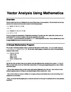
We can produce a topographical map of this region using ContourPlots : In[308]:=
Clearh, x, y hx_, y_ : 10 2 x y 3 x ^ 2 4 y ^ 2 18 x 28 y 112 ContourPlothx, y, x, 5, 2, y, 0, 8
Out[310]=
(Type this into your notebook and play with the image a bit; try the plot with different limits for x and y; scroll your mouse over the contour lines; read the classnote on gradient to see how to add contour lines to your own program.) We know that the gradient of h (x, y) will give us the magnitude and direction of increase at any point on the hill. Let' s compute grad h, and then plot the corresponding vector field : In[314]:= Out[314]=
Gradhx, y, Cartesianx, y, z 10 18 6 x 2 y, 10 28 2 x 8 y, 0
graddivcurl.nb
In[315]:=
3
VectorPlot1, 2, x, 5, 3, y, 0, 8 8
6
Out[315]=
4
2
0 -4
-2
0
2
The length and direction of each arrow shows the properties of the gradient at each point in the plotted region. Notice that the gradient seems to approach zero in the region of (-2, 3). What is the physical meaning of this? Let' s see if we can verify your answer doing the calculation : In[316]:=
Out[316]=
SolveDhx, y, x 0, Dhx, y, y 0, x, y x 2, y 3
We use Solve to solve two equations simultaneously; we use braces since we have a list of two equations. Each equation derives from applying the conditions for finding an extremum to our h (x, y) function; in other words, we take the partial derivates of h with respect to x and y respectively, set both equations to zero, and find that the peak of the hill occurs at coordinates (-2, 3). If you are not familiar with taking derivatives using Mathematica, use the doc center to learn more about differentiation in Mathematica. Finally, let' s consider a three dimensional flow field and study its vector properties. Consider a river flowing between parallel banks that are two units apart; consider also the depth of the river is 1/2 unit. A semi - realistic description of the velocity vector of this river is : ` v = -y^2 + 2 y 2 z x
4
graddivcurl.nb
Here, we are defining downstream as the x direction; the velocity is all downstream, but the magnitude of velocity depends on the y and z coordinates of the fluid position. We can plot this vector field : In[322]:=
VectorPlot3Dy^2 2 y z, 0, 0, x, 0, 2, y, 0, 2, z, 0, 1 2 2
1
0
0.6
0.4 Out[322]=
0.2
0.0 -0.2 0 1
2
This is a vector field that has a curl, meaning a small paddlewheel or leaf will spin in this flow field : curl Curl y ^ 2 2 y z, 0, 0, Cartesianx, y, z
Out[323]=
0, 2 y y2 , 2 2 y z
and we plot the curl field :
graddivcurl.nb
In[328]:=
VectorPlot3D0, 2 y y ^ 2, 2 2 y z, x, 0, 2, y, 0, 2, z, 0, 0.5 2
1
0
0.6
0.4 Out[328]=
0.2
0.0
-0.2 0
1
2
Can you explain why the direction of the angular velocity points in opposite directions on the opposite banks?
5