We describe four MATLAB classes for tensor manipulations that can be used for
fast algorithm prototyping. The tensor class extends the functionality of ...
MATLAB Tensor Classes for Fast Algorithm Prototyping BRETT W. BADER and TAMARA G. KOLDA Sandia National Laboratories
Tensors (also known as multidimensional arrays or N -way arrays) are used in a variety of applications ranging from chemometrics to psychometrics. We describe four MATLAB classes for tensor manipulations that can be used for fast algorithm prototyping. The tensor class extends the functionality of MATLAB’s multidimensional arrays by supporting additional operations such as tensor multiplication. The tensor as matrix class supports the “matricization” of a tensor, i.e., the conversion of a tensor to a matrix (and vice versa), a commonly used operation in many algorithms. Two additional classes represent tensors stored in decomposed formats: cp tensor and tucker tensor. We describe all of these classes and then demonstrate their use by showing how to implement several tensor algorithms that have appeared in the literature. Categories and Subject Descriptors: G.4 [Mathematics of Computing]: Mathematical Software—Algorithm Design and Analysis; G.1.m [Mathematics of Computing]: Numerical Analysis—Miscellaneous General Terms: Algorithms Additional Key Words and Phrases: Higher-Order Tensors, Multilinear Algebra, N-Way Arrays, MATLAB
1.
INTRODUCTION
A tensor is a multidimensional or N -way array of data; Figure 1 shows a 3way array of size I1 × I2 × I3 . Tensors arise in many applications, including chemometrics [Smilde et al. 2004], signal processing [Chen et al. 2002], and image processing [Vasilescu and Terzopoulos 2002]. In this paper, we describe four MATLAB classes for manipulating tensors: tensor, tensor as matrix, cp tensor, and tucker tensor. MATLAB is a high-level computing environment that allows users to develop mathematical algorithms using familiar mathematical notation. In terms of higherorder tensors, MATLAB supports multidimensional arrays (MDAs). Allowed opAuthors’ address: Sandia National Laboratories, Albuquerque, NM 87185 and Livermore, CA 94551. Authors’ emails: {bwbader,tgkolda}@sandia.gov. This research was sponsored by the Mathematical, Information, and Computational Sciences Division at the United States Department of Energy and by Sandia National Laboratory, a multiprogram laboratory operated by Sandia Corporation, a Lockheed Martin Company, for the United States Department of Energy under contract DE–AC04–94AL85000. Permission to make digital/hard copy of all or part of this material without fee for personal or classroom use provided that the copies are not made or distributed for profit or commercial advantage, the ACM copyright/server notice, the title of the publication, and its date appear, and notice is given that copying is by permission of the ACM, Inc. To copy otherwise, to republish, to post on servers, or to redistribute to lists requires prior specific permission and/or a fee. c 20YY ACM 0098-3500/20YY/1200-0001 $5.00
ACM Transactions on Mathematical Software, Vol. V, No. N, Month 20YY, Pages 1–0??.
2
·
B. W. Bader and T. G. Kolda
Fig. 1.
i3
=
1, .
..
,I
3
i1 = 1, . . . , I1 i2 = 1, . . . , I2
A 3-way array
erations on MDAs include elementwise operations, permutation of indices, and most vector operations (like sum and mean) [The MathWorks, Inc. 2004b]. More complex operations, such as the multiplication of two MDAs, are not supported by MATLAB. This paper describes a tensor datatype that extends MATLAB’s MDA functionality to support tensor multiplication and more through the use of MATLAB’s class functionality [The MathWorks, Inc. 2004a]. Basic mathematical notation and operations for tensors, as well as the related MATLAB commands, are described in §2. Tensor multiplication receives its own section, §3, in which we describe both notation and how to multiply a tensor times a vector, a tensor times a matrix, and a tensor times another tensor. Conversion of a tensor to a matrix (and vice versa) via the tensor as matrix class is described in §4. A tensor may be stored in factored form as a sum of rank-1 tensors. There are two commonly accepted factored forms. The first was developed independently under two names: the CANDECOMP model of Carroll and Chang [1970] and the PARAFAC model of Harshman [1970]. Following the notation in Kiers [2000], we refer to this decomposition as the CP model. The second decomposition is the Tucker [1966] model. Both models, as well as the corresponding MATLAB classes cp tensor and tucker tensor, are described in §5. We note that these MATLAB classes serve a purely supporting role in the sense that these classes do not contain high-level algorithms—just the data types and their associated member functions. Thus, we view this work as complementary to those packages that provide algorithms for use with tensor data, e.g., the N -way toolbox for MATLAB by Andersson and Bro [2000]. We use the following notational conventions. Indices are denoted by lowercase letters and span the range from 1 to the uppercase letter of the index, e.g., n = 1, 2, . . . , N . We denote vectors by lowercase boldface letters, e.g., x; matrices by uppercase boldface, e.g., U; and tensors by calligraphic letters, e.g., A. Notation for tensor mathematics is still sometimes awkward. We have tried to be as standard as possible, relying on Harshman [2001] and Kiers [2000] for some guidance in this ACM Transactions on Mathematical Software, Vol. V, No. N, Month 20YY.
Tensor Classes
·
3
regard. Throughout the paper, we refer to numbered examples that the reader should run in MATLAB. These examples are located in the examples directory. Before running the examples, the user should change directories to the examples directory and run the setup script to set the path. The script runall runs all example scripts in sequence, and the file runall.out is a text file that shows sample output, useful for those who do not have MATLAB at hand or who wish to compare their output to ours. These methods have been tested on MATLAB version 7.0.1.24704 (R14) Service Pack 1. 2.
BASIC NOTATION & MATLAB COMMANDS FOR TENSORS
Let A be a tensor of dimension I1 × I2 × · · · × IN . The order of A is N . The nth dimension (or mode or way) of A is of size In . A scalar is a zeroth-order tensor. An n-vector is a first-order tensor of size n. An m × n matrix is a second-order tensor of size m × n. Of course, a single number could be a scalar, a 1-vector, a 1 × 1 matrix, etc. Similarly, an n-vector could be viewed as an n×1 matrix, or an m×n matrix could be viewed as a m×n×1 tensor. It depends on the context, and our tensor class explicitly tracks the context, as described in §2.2. We denote the index of a single element within a tensor by either subscripts or parentheses. Subscripts are generally used for indexing on matrices and vectors but can be confusing for the complex indexing that is sometimes required for tensors. In general, we use A(i1 , i2 , . . . , iN ) rather than Ai1 i2 ···iN . We use colon notation to denote the full range of a given index. The ith row of a matrix A is given by A(i, :), and the jth column is A(:, j). For higher-order tensors, the notation is extended in an obvious way, but the terminology is more complicated. Consider a 3rd-order tensor. In this case, specifying a single index yields a slice [Kiers 2000], which is a matrix in a specific orientation. So, A(i, :, :) yields the ith horizontal slice, A(:, j, :) the jth lateral slice, and A(:, :, k) the kth frontal slice; see Figure 2.
Horizontal A(i, :, :)
Lateral A(:, j, :) Fig. 2.
Frontal A(:, :, k)
Slices of a 3rd-order tensor.
On the other hand, A(:, j, k) yields a column vector, A(i, :, k) yields a row vector, and A(i, j, :) yields a so-called tube vector [Kroonenberg 2004]; see Figure 3. AlterACM Transactions on Mathematical Software, Vol. V, No. N, Month 20YY.
·
4
B. W. Bader and T. G. Kolda
natively, these are called column fibers, row fibers, and depth fibers, respectively [Kiers 2000]. In general, a mode-n fiber is specified by fixing all dimensions except the nth.
Mode-1 — Columns A(:, j, k)
Mode-2 — Rows A(i, :, k) Fig. 3.
2.1
Mode-3 — Tubes A(i, j, :)
Fibers of a 3rd-order tensor.
Creating a tensor object
In MATLAB, a higher-order tensor can be stored as an MDA. Our tensor class extends the capabilities of the MDA datatype. An array or MDA can be converted to a tensor as follows. T = tensor(A) or T = tensor(A,DIM) converts an array (scalar, vector, matrix, or MDA) to a tensor. Here A is the object to be converted and DIM specifies the dimensions of the object. A = double(T) converts a tensor to an array (scalar, vector, matrix, or MDA).
Run the script ex1 to see an example of converting an MDA to a tensor. 2.2
Tensors and size
Out of necessity, the tensor class handles sizes in a different way than the MATLAB arrays. Every MATLAB array has at least 2 dimensions; for example, a scalar is an object of size 1 × 1 and a column vector is an object of size n × 1. On the other hand, MATLAB drops trailing singleton dimensions for any object of order greater than 2. Thus, a 4 × 3 × 1 object has a reported size of 4 × 3. Our MATLAB tensor class explicitly stores trailing singleton dimensions; run the script ex2 to illustrate this. Furthermore, the tensor class allows for tensors of order zero (for a scalar) or one (for a vector); run the script ex3 to see this behavior. The function order returns the mathematical concept of order for a tensor, while the function ndims returns an algorithmic notion of the dimensions of a tensor, which is useful ACM Transactions on Mathematical Software, Vol. V, No. N, Month 20YY.
Tensor Classes
·
5
for determining the number of subscripts capable of accessing all of the elements in the data structure (i.e., 1 for the case of a scalar or vector). Note that the script ex3 also shows that the whos command does not report the correct sizes in the zero- or one-dimensional cases. The tensor constructor argument DIM must be specified whenever the order is intended to be zero or one or when there are trailing singleton dimensions. 2.3
Accessors
In MATLAB, indexing a tensor is the same as indexing a matrix:
A(i1,i2,...,iN) returns the (i1 , i2 , . . . , iN ) element of A.
Recall that A(:, :, k) denotes the kth frontal slice. straightforward:
The MATLAB notation is
A(:,:,k) returns the kth submatrix (as a tensor) along the third dimension of the tensor A.
The script ex4 shows that the accessors for a tensor work generally the same as they would for an MDA. 2.4
General functionality
In general, a tensor object will behave exactly as an MDA for all functions that are defined for an MDA; a list of these functions is provided in Figure 4.
• • • • • • • •
A + B or plus(A,B) A - B or minus(A,B) -A or uminus(A) +A or uplus(A) A.*B or times(A,B) A./B or rdivide(A,B) A.\B or ldivide(A,B) A.^B or power(A,B)
Fig. 4.
• • • • • • • • •
A < B or lt(A,B) A > B or gt(A,B) A = B or ge(A,B) A ~= B or ne(A,B) A == B or eq(A,B) A & B or and(A,B) A | B or or(A,B) ~A or not(A)
Functions that behave identically for tensors and multidimensional arrays.
ACM Transactions on Mathematical Software, Vol. V, No. N, Month 20YY.
·
6
3.
B. W. Bader and T. G. Kolda
TENSOR MULTIPLICATION
Notation for tensor multiplication is very complex. The issues have to do with specifying which dimensions are to be multiplied and how the dimensions of the result should be ordered. We approached this problem by developing notation that can be expressed easily by MATLAB. We describe three types of tensor multiplication: tensor times a matrix (§3.1), tensor times a vector (§3.2), and tensor times a tensor (§3.3). Both tensor times a matrix and tensor times a vector provide special instances of the functionality that is provided by the tensor times tensor case. 3.1
Multiplying a tensor times a matrix
The first question we consider is how to multiply a tensor times a matrix. With matrix multiplication, the specification of which dimensions should be multiplied is straightforward—it is always the inner product of the rows of the first matrix with the columns of the second matrix. A transpose on an argument swaps the rows and columns. Because tensors may have an arbitrary number of dimensions, the situation is more complicated. In this case, we need to specify which dimension of the tensor is multiplied by the columns (or rows) of the given matrix. The adopted solution is the n-mode product [De Lathauwer et al. 2000a]. Let A be an I1 × I2 × · · · × IN tensor, and let U be an Jn × In matrix. Then the n-mode product of A and U is denoted by A ×n U, and defined (elementwise) as (A ×n U)(i1 , . . . , in−1 , jn , in+1 , . . . , iN ) =
In X
A(i1 , i2 , . . . , iN ) B(jn , in ).
in =1
The result is a tensor of size I1 × · · · × In−1 × Jn × In+1 × · · · × IN . Some authors call this operation the mode-n inner product and denote it as A •n U (see, e.g., Comon [2001]). To understand n-mode multiplication in terms of matrices (i.e., order-2 tensors), suppose A is m × n, U is m × k, and V is n × k. It follows that A ×1 UT = UT A
and A ×2 VT = AV.
Further, the matrix SVD can be written as A = UΣVT = Σ ×1 U ×2 V. The following MATLAB commands can be used to calculate n-mode products.
B = ttm(A,U,n) calculates “tensor times matrix” in mode-n, i.e., B = A ×n U. B = ttm(A,{U,V},[m,n]) calculates two sequential n-mode products in the specified modes, i.e., B = A ×m U ×n V. ACM Transactions on Mathematical Software, Vol. V, No. N, Month 20YY.
Tensor Classes
·
7
The n-mode product satisfies the following property [De Lathauwer et al. 2000a]. Let A be a tensor of size I1 × I2 × · · · × IN . If U ∈ RJm ×Im and V ∈ RJn ×In , then A ×m U ×n V = A ×n V ×m U.
(1)
Run the script ex5 to see n-mode products that demonstrates this property, and run ex6 to revisit the same example using cell arrays to calculate the n-mode products. It is often desirable to calculate the product of a tensor and a sequence of matrices. Let A be an I1 × I2 × · · · × IN tensor, and let U(n) denote a Jn × In matrix for n = 1, . . . , N . Then the sequence of products B = A ×1 U(1) ×2 U(2) · · · ×N U(N )
(2)
is of size J1 × J2 × · · · × JN . We propose new, alternative notation for this operation that is consistent with the MATLAB notation for cell arrays: B = A × {U}. This mathematical notation will prove useful in presenting some algorithms, as shown in §6. The following equivalent MATLAB commands can be used to calculate n-mode products with a sequence of matrices. B = ttm(A,{U1,U2,...,UN}, [1:N]) calculates B = A ×1 U(1) ×2 U(2) · · · ×n U(N ) . Here Un is a MATLAB matrix representing U(n) . B = ttm(A,U) calculates B = A × {U}. Here U = {U1,U2,. . . ,UN} is a MATLAB cell array and Un is as described above.
Another frequently used operation is multiplying by all but one of a sequence of matrices: B = A ×1 U(1) · · · ×n−1 U(n−1) ×n+1 U(n+1) · · · ×N U(N ) . We propose new, alternative notation for this operation: B = A ×−n {U}. This notation will prove useful in presenting some algorithms in §6. The following MATLAB commands can be used to calculate n-mode products with all but one of a sequence of matrices. B = ttm(A,U,-n) calculates B = A ×−n {U}. Here U = {U1,U2,. . . ,UN} is a MATLAB cell array; the nth cell is simply ignored in the computation. Note that B = ttm(A,{U1,. . . ,U4,U6,. . . ,U9},[1:4,6:9]) is equivalent to B = ttm(A,U,-5) where U={U1,. . . ,U9} ; both calculate B = A ×−5 {U}. ACM Transactions on Mathematical Software, Vol. V, No. N, Month 20YY.
8
·
3.2
Multiplying a tensor times a vector
B. W. Bader and T. G. Kolda
In our opinion, one source of confusion in n-mode multiplication is what to do to the singleton dimension in mode n that is introduced when multiplying a tensor times a vector. If the singleton dimension is dropped (as is sometimes desired), then the commutativity of the multiplies (1) outlined in the previous section no longer holds because the order of the intermediate result changes and ×n or ×m applies to the wrong mode. Although one can usually determine the correct order of the result via the context of the equation, it is impossible to do this automatically in MATLAB in any robust way. Thus, we propose an alternate name and notation in the case when the newly introduced singleton dimension indeed should be dropped. Let A be an I1 × I2 × · · · × IN tensor, and let b be an In -vector. We propose that the contracted n-mode product, which drops the nth singleton dimension, be denoted by ¯ n b. A× The result is of size I1 × · · · × In−1 × In+1 × · · · × IN . Note that the order of the result is N − 1, one less than the original tensor. The entries are computed as: ¯ n u)(i1 , . . . , in−1 , in+1 , . . . , iN ) = (A ×
In X
A(i1 , i2 , . . . , iN ) u(in ).
in =1
The following MATLAB command computes the contracted n-mode product. B = ttv(A,u,n) calculates “tensor times vector” in mode-n, i.e., ¯ n u. B = A× ¯ n u and A ×n uT produce identical results except for the order Observe that A × ¯ n u is of size I1 × · · · × In−1 × In+1 × · · · × IN , and shape of the results; that is, A × T whereas A ×n u is of size I1 × · · · × In−1 × 1 × In+1 × · · · × IN . Run ex7 for a comparison of ttv and ttm. Because the contracted n-mode product drops the nth singleton dimension, it is no longer true that multiplication is commutative; i.e., ¯ m u) × ¯ n v 6= (A × ¯ n v) × ¯ m u. (A × However, a different statement about commutativity may be made. If we assume m < n, then ¯ m u) × ¯ n−1 v = (A × ¯ n v) × ¯ m u. (A × For the sake of clarity in a sequence of contracted n-mode products, we assume that the order reduction happens after all products have been computed. This assumption obviates the need to explicitly place parentheses in an expression and appropriately decrement any n-mode product indices. In other words, ( ¯ m u) × ¯n v (A × : m > n, ¯m u× ¯n v ≡ A× (3) ¯ ¯ (A ×m u) ×n−1 v : m < n. ACM Transactions on Mathematical Software, Vol. V, No. N, Month 20YY.
Tensor Classes
·
9
As before with matrices, it is often useful to calculate the product of a tensor and a sequence of vectors; e.g., ¯ 1 u(1) × ¯ 2 u(2) · · · × ¯ N u(N ) B = A× or ¯ 1 u(1) · · · × ¯ n−1 u(n−1) × ¯ n+1 u(n+1) · · · × ¯ N u(N ) . B = A× We propose the following alternative notation for these two cases: ¯ {u} B = A× and ¯ −n {u}, B = A× respectively. In practice, one must be careful when calculating a sequence of contracted n-mode products to perform the multiplications starting with the highest mode and proceed sequentially to the lowest mode. The following MATLAB commands automatically sort the modes in the correct order. ¯ 1 u(1) × ¯ 3 u(3) where u1 and B = ttv(A, u1,u3, [1,3]) computes B = A × (1) (3) u3 correspond to vectors u and u , respectively. ¯ {u} where u is a cell array whose nth B = ttv(A,u) computes B = A × entry is the vector u(n) . ¯ −n {u}. B = ttv(A,u,-n) computes B = A ×
Note that the result of the second expression is a scalar, and the result of the third expression is a vector of size In ; run ex8 for examples of a tensor times a sequence of vectors. 3.3
Multiplying a tensor times another tensor
The last category of tensor multiplication to consider is the product of two tensors. We consider three general scenarios for tensor-tensor multiplication: outer product, contracted product, and inner product. The outer product of two tensors is defined as follows. Let A be of size I1 × · · · × IM , and let B be of size J1 × · · · × JN . The outer product A ◦ B is of size I1 × · · · × IM × J1 × · · · × JN and is given by (A ◦ B)(i1 , . . . iM , j1 , . . . , jN ) = A(i1 , . . . , iM )B(j1 , . . . , jN ). In MATLAB, the command is as follows.
C= ttt(A,B) computes “tensor times tensor”; i.e., the outer product C = A ◦ B. ACM Transactions on Mathematical Software, Vol. V, No. N, Month 20YY.
10
·
B. W. Bader and T. G. Kolda
Run ex9 to see an example the outer product. The contracted product of two tensors is a generalization of the tensor-vector and tensor-matrix multiplications discussed in the previous two subsections. The key distinction is that the modes to be multiplied and the ordering of the resulting modes is handled specially in the matrix and vector cases. In this general case, let A be of size I1 ×· · ·×IM ×J1 ×· · ·×JN and B be of size I1 ×· · ·×IM ×K1 ×· · ·×KP . We can multiply both tensors along the first M modes, and the result is a tensor of size J1 × · · · × JN × K1 × · · · × KP , given by hA, Bi{1,...,M ;1,...,M } (j1 , . . . jN , k1 , . . . , kP ) = I1 X
IM X
···
A(i1 , . . . , iM , j1 , . . . , jN ) B(i1 , . . . , iM , k1 , . . . , kP ).
iM =1
i1 =1
With this notation, the modes to be multiplied are specified in the subscripts that follow the angle brackets. The remaining modes are ordered such that those from A come before B, which is different from the tensor-matrix product case considered above where the leftover matrix dimension of B replaces In rather than moved to the end. In MATLAB, the command for the tensor contracted product is as follows. C = ttt(A,B,[1:M],[1:M]) computes C = hA, Bi{1,...,M ;1,...,M } .
The arguments specifying the modes of A and the modes of B for contraction need not be consecutive, as shown in the previous example. However, the sizes of the corresponding dimensions must be equal. That is, if we call ttt(A,B,ADIMS,BDIMS) then size(A,ADIMS) and size(B,BDIMS) must be identical. Run ex10 to see examples of contracted products. The inner product of two tensors requires that both tensors have equal dimensions. Assuming both are of size I1 × I2 × · · · × IN , their inner product is given by hA, Bi =
I1 X I2 X
···
i1 =1 i2 =1
IN X
A(i1 , i2 , . . . , iN ) B(i1 , i2 , . . . , iN ).
iN =1
In MATLAB this is accomplished via either of the following commands. ttt(A,B,[1:N]) or A*B calculates hA, Bi; the result is a scalar.
See ex11 for examples of using each notation. Using this definition of inner product, the Frobenius norm of a tensor is then given by 2
kAkF = hA, Ai =
I1 X I2 X i1 =1 i2 =1
···
IN X
A(i1 , i2 , . . . , iN )2 .
iN =1
ACM Transactions on Mathematical Software, Vol. V, No. N, Month 20YY.
Tensor Classes
·
11
In MATLAB the norm can be calculated as follows. norm(A) calculates kAkF , the Frobenius norm of a tensor.
4.
MATRICIZE: TRANSFORMING A TENSOR INTO A MATRIX
It is often useful to rearrange the elements of a tensor so that they form a matrix. Although many names for this process exist, we call it “matricizing,” following Kiers [2000], because matricizing a tensor is analogous to vectorizing a matrix. De Lathauwer et al. [2000a] call this process “unfolding.” It is sometimes also called “flattening” (see, e.g., [Vasilescu and Terzopoulos 2002]). 4.1
General Matricize
Let A be an I1 × I2 × · · · × IN tensor, and suppose we wish to rearrange it to be a matrix of size J1 × J2 . Clearly, the number of entries QN in the matrix must equal the number of entries in the tensor; in other words, n=1 In = J1 J2 . Given J1 and J2 satisfying the above property, the mapping can be done any number of ways so long as we have a one-to-one mapping π such that π : {1, . . . , I1 } × {1, . . . , I2 } × · · · × {1, · · · , IN } → {1, . . . , J1 } × {1, . . . , J2 }. The tensor as matrix class supports the conversion of a tensor to a matrix as follows. Let the set of indices be partitioned into two disjoint subsets: {1, . . . , N } = {r1 , . . . , rK } ∪ {c1 , . . . , cL }. The set {r1 , . . . , rK } defines those indices that will be mapped to the row indices of the resulting matrix and the set {c1 , . . . , cL } defines those indices that will likewise be mapped to the column indices. In this case, J1 =
K Y k=1
Irk
and J2 =
L Y
Ic` .
`=1
Then we define π(i1 , i2 , . . . , iN ) = (j1 , j2 ) where K k−1 L `−1 X Y X Y (irk − 1) (ir` − 1) j1 = 1 + Irkˆ and j2 = 1 + Ir`ˆ . k=1
ˆ k=1
`=1
ˆ `=1
Note that the sets {r1 , . . . , rK } and {c1 , . . . , cL } can be in any order and are not necessarily ascending. The following MATLAB commands convert a tensor to a matrix, and ex12 shows some examples. A = tensor as matrix(T,RDIMS) matricizes T such that the dimensions (or modes) specified in RDIMS map to the rows of the matrix (in the order given), and the remaining dimensions (in ascending order) map to the columns. A = tensor as matrix(T,RDIMS,CDIMS) matricizes T such that the dimensions specified in RDIMS map to the rows of the matrix, and the dimensions specified in CDIMS map to the columns, both in the order given. ACM Transactions on Mathematical Software, Vol. V, No. N, Month 20YY.
·
12
B. W. Bader and T. G. Kolda
A tensor as matrix object can be converted to a matrix as follows. B = double(A) converts the tensor as matrix object to a matrix.
Also, the size of the corresponding tensor, the tensor indices corresponding to the matrix rows, and tensor indices corresponding to the matrix columns can be extracted as follows. sz = A.tsize gives the size of the corresponding tensor. ridx = A.rindices gives the indices that have been mapped to the rows, i.e., {r1 , . . . , rK }. cidx = A.cindices gives the indices that have been mapped to the columns, i.e., {c1 , . . . , cL }.
With overloaded functions in MATLAB, the tensor as matrix class allows multiplication between tensors and/or matrices. More precisely, mtimes(A,B) is called for the syntax A * B when A or B is a tensor as matrix object. The result is another tensor as matrix object that can be converted back into a tensor object, as described below. The multiplication is analogous to the functionality provided by ttt for multiplying two tensor objects. Run ex13 to see tensor-tensor multiplication using tensor as matrix objects. Given a tensor as matrix object, we can automatically rearrange its entries back into a tensor by passing the tensor as matrix object into the constructor for the tensor class. The tensor as matrix class contains the mode of matricization and original tensor dimensions, making the conversion transparent to the user. The following MATLAB command can convert a matrix to a tensor, and ex14 shows such a conversion. tensor(A) creates a tensor from A, which is a tensor as matrix object.
4.2
Mode-n Matricize
Typically, a tensor is matricized so that all of the fibers associated with a particular single dimension are aligned as the columns of the resulting matrix. In other words, we align the fibers of dimension n of a tensor A to be the columns of the matrix. This is a special case of the general matricize where only one dimension is mapped to the rows, so K = 1 and {r1 } = {n}. The resulting matrix is typically denoted by A(n) . The columns can be ordered in any way. Two standard, but different, orderings are used by De Lathauwer et al. [2000a] and Kiers [2000]. Both are cyclic, but ACM Transactions on Mathematical Software, Vol. V, No. N, Month 20YY.
Tensor Classes
·
13
the order is reversed. For De Lathauwer et al. [2000a], the ordering is given by {c1 , . . . , cL } = {n −1, n −2, . . . , 1, N, N −1, . . . , n + 1}, and we refer to this ordering as backward cyclic or “bc” for short. For Kiers [2000], the ordering is given by {c1 , . . . , cL } = {n + 1, n + 2, . . . , N, 1, 2, . . . , n − 1}, and we refer to this ordering as forward cyclic or “fc” for short. Figure 5 shows the backward cyclic ordering and Figure 6 shows the forward cyclic ordering. I2
A(1)
A I1
I3
I1 I2
I3
I3
A(2)
A I2
I3
I1 I2
I1
I1
A(3)
A I3
I3
I1 I2 Fig. 5.
I2 Backward cyclic matricizing a 3-way tensor.
The following MATLAB commands can convert a tensor to a matrix according to the two definitions above, and ex15 shows two examples of matricizing a tensor.
tensor as matrix(T,n,’bc’) computes T(n) , i.e., matricizing T using a backward cyclic ordering. The equivalent general command is tensor as matrix(T,n, [n-1:-1:1 ndims(T):-1:n+1]). tensor as matrix(T,n,’fc’) computes T(n) , i.e., matricizing T using a forward cyclic ordering. The equivalent general command is tensor as matrix(T,n, [n+1:ndims(T) 1:n-1]).
One benefit of matricizing is that tensors stored in matricized form may be manipulated as matrices, reducing n-mode multiplication, for example, to a matrix-matrix operation. If B = A ×n M, then B(n) = MA(n) . ACM Transactions on Mathematical Software, Vol. V, No. N, Month 20YY.
14
·
B. W. Bader and T. G. Kolda I3
A(1)
A I1
I3
I1 I2
I2
I1
A(2)
A I2
I3
I1 I2
I3
I2
A(3)
A I3
I3
I1 I2 Fig. 6.
I1 Forward cyclic matricizing a 3-way tensor.
Moreover, the series of n-mode products in (2), when written as a matrix formulation, can be expressed as a series of Kronecker products involving the U matrices. Consider the ordering of the tensor dimensions that map to the column space of the matrix (e.g., for forward cyclic ordering about mode-3 on a 4th-order tensor; then {r1 } = {3} and {c1 , c2 , c3 } = {4, 1, 2}). The series of n-mode products in (2) is given by � �T B(n) = U(n) A(n) U(cn−1 ) ⊗ U(cn−2 ) ⊗ · · · ⊗ U(c1 ) . The script ex16 shows an example of computing the series of n-mode products using tensor as matrix and Kronecker products. The tensor as matrix object is converted into a standard MATLAB matrix for matrix-matrix multiplication, and the result must be converted back to a tensor with further matrix manipulations. Because this approach requires that the user code some lower level details, this example highlights the simplicity of the tensor class, which accomplishes the same computation in one function call to ttm. 5.
DECOMPOSED TENSORS
As mentioned previously, we have also created two additional classes to support the representation of tensors in decomposed form, that is, as the sum of rank-1 tensors. A rank-1 tensor is a tensor that can be written as the outer product of vectors, i.e., A = λ u(1) ◦ u(2) ◦ · · · ◦ u(N ) , where λ is a scalar and each u(n) is an In -vector, for n = 1, . . . , N . The ◦ symbol denotes the outer product; so, in this case, the (i1 , i2 , . . . , iN ) entry of A is given ACM Transactions on Mathematical Software, Vol. V, No. N, Month 20YY.
Tensor Classes
·
15
by (1)
(2)
(N )
A(i1 , i2 , . . . , iN ) = λ ui1 ui2 · · · uiN , where ui denotes the ith entry of vector u. We focus on two different tensor decompositions: CP and Tucker. 5.1
CP tensors
Recall that “CP” is shorthand for CANDECOMP [Carroll and Chang 1970] and PARAFAC [Harshman 1970], which are identical decompositions that were developed independently for different applications. The CP decomposition is a weighted sum of rank-1 tensors, given by A=
K X
(1)
(2)
(N )
λk U:k ◦ U:k ◦ · · · ◦ U:k .
(4)
k=1
Here λ is a vector of size K and each U(n) is a matrix of size In ×K, for n = 1, . . . , N . (n) Recall that the notation U:k denotes the kth column of the matrix U(n) . The following MATLAB command creates a CP tensor. T = cp tensor(lambda,U) creates a cp tensor object. Here lambda is a K-vector and U is a cell array whose nth entry is the matrix U (n) with K columns. T = cp tensor(U) creates a cp tensor object where all the λk ’s are assumed to be one. A CP tensor can be converted to a dense tensor as follows, and ex17 provides an example. B = full(A) converts a cp tensor object to a tensor object.
Addition and subtraction of CP tensors is handled in a special manner. The λ’s and U(n) ’s are concatenated. To add or subtract two CP tensors (of the same order and size), use the + and - signs. An example is shown in ex18 A + B computes the sum of two CP tensors. A - B computes the difference of two CP tensors.
To determine the value of K for a CP tensor, execute the following MATLAB command. r = length(T.lambda) returns the number of components of the tensor T.
ACM Transactions on Mathematical Software, Vol. V, No. N, Month 20YY.
·
16
5.2
B. W. Bader and T. G. Kolda
Tucker tensors
The Tucker decomposition [Tucker 1966], also called a Rank-(K1 , K2 , . . . , KN ) decomposition [De Lathauwer et al. 2000b], is another way of summing decomposed tensors and is given by A=
K2 K1 X X k1 =1 k2 =1
···
KN X
(1)
(2)
(N )
λ(k1 , k2 , . . . , kN ) U:k1 ◦ U:k2 ◦ · · · ◦ U:kN .
(5)
kN =1
Here λ is itself a tensor of size K1 × K2 × · · · × KN , and each U(n) is a matrix (n) of size In × Kn , for n = 1, . . . , N . As before, the notation U:k denotes the kth (n) column of the matrix U . The tensor λ is often called the “core array” or “core tensor.” A Tucker tensor can be created in MATLAB as follows, and ex19 shows an example.
T = tucker tensor(lambda,U) where lambda is a K1 × K2 × · · · × KN tensor and U is a cell array whose nth entry is a matrix with Kn columns.
A Tucker tensor can be converted to a dense tensor as follows. B = full(A) converts a tucker tensor object to a tensor object.
6.
EXAMPLES
We demonstrate the use of the tensor, cp tensor, and tucker tensor classes for algorithm development by implementing the higher-order generalizations of the power method and orthogonal iteration presented by De Lathauwer et al. [2000b]. The first example is the higher-order power method, Algorithm 3.2 of De Lathauwer et al. [2000b], which is a multilinear generalization of the best rank-1 approximation problem for matrices. This is also the same as the Alternating Least Squares algorithm for fitting a rank-1 CP model. The best rank-1 approximation problem is that, given a tensor A, we want to find a B of the form B = λ u(1) ◦ u(2) ◦ · · · ◦ u(N ) , such that k A−B k is as small as possible. The higher-order power method computes a B that approximately solves this problem. Essentially, this method works as follows. It fixes all u-vectors except u(1) and then solves for the optimal u(1) , likewise for u(2) , u(3) , and so on, cycling through the indices until the specified number of iterations is exhausted. In Figure 7, we show the algorithm using our new notation, and the file examples/hopm.m shows the MATLAB code that implements the algorithm. Run ex20 to find a rank-1 CP approximation to a tensor using the higher-order power method ACM Transactions on Mathematical Software, Vol. V, No. N, Month 20YY.
Tensor Classes
·
17
Higher-Order Power Method In: A of size I1 × I2 × · · · × IN . Out: B of size I1 × I2 × · · · × IN , an estimate of the best rank-1 approximation of A. (n)
(1) Compute initial values: Let u0 be the dominant left singular vector of A(n) for n = 2, . . . , N . (2) For k = 0, 1, 2, . . . (until converged), do: For n = 1, . . . , N , do: (n) ¯ −n {uk }. ˜ k+1 = A × u
˜ k+1 λk+1 = u (n)
(n)
(n)
(n)
(n)
˜ k+1 /λk+1 uk+1 = u (3) Let λ = λK and {u} = {uK }, where K is the index of the final result of step 2. (4) Set B = λ u(1) ◦ u(2) ◦ · · · ◦ u(n) .
Fig. 7. Higher-order power method algorithm of De Lathauwer, De Moor, and Vandewalle using the proposed notation. In this illustration, subscripts denote iteration number.
The second example is the higher-order orthogonal iteration, which is the multilinear generalization of the best rank-R approximation problem for matrices. Algorithm 4.2 in [De Lathauwer et al. 2000b] is the higher-order orthogonal iteration and finds the best rank-(R1 , R2 , . . . , RN ) approximation of a higher-order tensor. We have reproduced this algorithm in Figure 8 using our new notation. Our corresponding MATLAB implementation is listed in examples/hooi.m. Run ex21 to generate a rank-(1,1,1) Tucker approximation to the same tensor used in ex20 , and note that the answers are identical. Run ex22 to generate a rank-(2,2,1) Tucker approximation and note that the quality of the approximation has improved. Run ex23 to generate a model with a core array that is the same size as the original tensor and observe that the approximation is equal to the original tensor. 7.
CONCLUSIONS
We have described four new MATLAB classes for manipulating dense and factored tensors. These classes extend MATLAB’s built-in capabilities for multidimensional arrays in order to facilitate rapid algorithm development when dealing with tensor datatypes. The tensor class simplifies the algorithmic details for implementing numerical methods for higher-order tensors by hiding the underlying matrix operations. It was previously the case that users had to know how to appropriately reshape the tensor into a matrix, execute the desired operation using matrix commands, and then appropriately reshape the result into a tensor. This can be nonintuitive and cumbersome, and we believe using the tensor class will be much simpler. The tensor as matrix class offers a way to convert a higher-order tensor into a matrix. Many existing algorithms in the literature that deal with tensors rely on matrix-matrix operations. The tensor as matrix functionality offers a means ACM Transactions on Mathematical Software, Vol. V, No. N, Month 20YY.
18
·
B. W. Bader and T. G. Kolda
Higher-Order Orthogonal Iteration In: A of size I1 × I2 × · · · × IN and desired rank of output. Out: B of size I1 × I2 × · · · × IN , an estimate of the best rank-(R1 , R2 , . . . , RN ) approximation of A. (n)
(1) Compute initial values: Let U0 ∈ RIn ×Rn be an orthonormal basis for the dominant Rn -dimensional left singular subspace of A(n) for n = 2, . . . , n. (2) For k = 0, 1, 2, . . . (until converged), do: For n = 1, . . . , N , do: U˜ = A ×−n {UT k} Let W
of size In × Rn solve:
max U˜ ×n WT subject to WT W = I. (n)
Uk+1 = W. (3) Let {U} = {UK }, where K is the index of the final result of step 2. (4) Set λ = A × {UT }. (5) Set B = λ × {U}.
Fig. 8. Higher-order orthogonal iteration algorithm of De Lathauwer, De Moor, and Vandewalle using the proposed notation. In this illustration, subscripts denote iteration number.
to implement these algorithms more easily, without the difficulty of reshaping and permuting tensor objects to the desired shape. The tucker tensor and cp tensor classes give users an easy way to store and manipulate factored tensors, as well as the ability to convert such tensors into non-factored (or dense) format. At this stage, our MATLAB implementations are not optimized for performance or memory usage; however, we have striven for consistency and ease-of-use. In the future, we plan to further enhance these classes and add additional functionality. Over the course of this code development effort, we have relied on published notation, especially from Kiers [2000] and De Lathauwer et al. [2000b]. To address ambiguities that we discovered in the class development process, we have proposed extensions to the existing mathematical notation, particularly in the area of tensor multiplication, that we believe more clearly denote mathematical concepts that were difficult to write succinctly with the existing notation. We have demonstrated our new notation and MATLAB classes by revisiting the higher-order power method and the higher-order orthogonal iteration method from [De Lathauwer et al. 2000b]. In our opinion, the resulting algorithm and code is more easily understood using our consolidated notation and MATLAB classes. Acknowledgments For their many helpful suggestions, we gratefully acknowledge the participants at the Tensor Decompositions Workshop held at the American Institute of Mathematics (AIM) in Palo Alto, CA on July 19–23, 2004. We also thank AIM and the National Science Foundation for sponsoring the workshop. We also thank the refACM Transactions on Mathematical Software, Vol. V, No. N, Month 20YY.
Tensor Classes
·
19
erees for carefully reading the manuscript and code and for suggesting many useful improvements and corrections. REFERENCES Andersson, C. A. and Bro, R. 2000. The N -way toolbox for MATLAB. Chemometrics & Intelligent Laboratory Systems 52, 1, 1–4. http://www.models.kvl.dk/source/nwaytoolbox/. Carroll, J. D. and Chang, J. J. 1970. Analysis of individual differences in multidimensional scaling via an n-way generalization of ’Eckart-Young’ decomposition. Psychometrika 35, 283– 319. Chen, B., Petropolu, A., and De Lathauwer, L. 2002. Blind identification of convolutive mim systems with 3 sources and 2 sensors. Applied Signal Processing (Special Issue on Space-Time Coding and Its Applications, Part II) 5, 487–496. Comon, P. 2001. Tensor decompositions. In Mathematics in Signal Processing V, J. G. McWhirter and I. K. Proudler, Eds. Oxford University Press, Oxford, UK, 1–24. De Lathauwer, L., De Moor, B., and Vandewalle, J. 2000a. A multilinear singular value decomposition. SIAM J. Matrix Anal. Appl. 21, 4, 1253–1278. De Lathauwer, L., De Moor, B., and Vandewalle, J. 2000b. On the best rank-1 and rank(R1 , R2 , . . . , RN ) approximation of higher-order tensors. SIAM J. Matrix Anal. Appl. 21, 4, 1324–1342. Harshman, R. A. 1970. Foundations of the PARAFAC procedure: Models and conditions for an “explanatory” multi-modal factor analysis. UCLA working papers in phonetics 16, 1–84. Harshman, R. A. 2001. An index formulism that generalizes the capabilities of matrix notation and algebra to n-way arrays. J. Chemometrics 15, 689–714. Kiers, H. A. L. 2000. Towards a standardized notation and terminology in multiway analysis. J. Chemometrics 14, 105–122. Kroonenberg, P. 2004. Applications of three-mode techniques: Overview, problems, and prospects. Presentation at the 2004 AIM Tensor Decompositions Workshop, Palo Alto, California, July 19-23, 2004. http://csmr.ca.sandia.gov/∼tgkolda/tdw2004/Kroonenberg%20-% 20Talk.pdf. Smilde, A., Bro, R., and Geladi, P. 2004. Multi-way Analysis: Applications in the Chemical Sciences. Wiley. The MathWorks, Inc. 2004a. Documentation: MATLAB: Programming: Classes and objects. http://www.mathworks.com/access/helpdesk/help/techdoc/matlab prog/ch11 mat.html. The MathWorks, Inc. 2004b. Documentation: MATLAB: Programming: Multidimensional arrays. http://www.mathworks.com/access/helpdesk/help/techdoc/matlab prog/ch dat32. html#39663. Tucker, L. R. 1966. Some mathematical notes on three-mode factor analysis. Psychometrika 31, 279–311. Vasilescu, M. A. O. and Terzopoulos, D. 2002. Multilinear analysis of image ensembles: Tensorfaces. In Proc. 7th European Conference on Computer Vision (ECCV’02), Copenhagen, Denmark, May 2002. Lecture Notes in Computer Science, vol. 2350. Springer-Verlag, 447–460.
ACM Transactions on Mathematical Software, Vol. V, No. N, Month 20YY.