Matrix Ansatz, lattice paths and rook placements

S. Corteel1 and M. Josuat-Vergès1† and T. Prellberg 2 and M. Rubey‡3 1

LRI, CNRS and Université Paris-Sud, Bâtiment 490, 91405 Orsay, France

2

School of Mathematical Sciences, Queen Mary, University of London, Mile End Road, London E1 4NS, United Kingdom 3

Institut für Algebra, Zahlentheorie und Diskrete Mathematik, Leibniz Universität Hannover, Welfengarten 1, 30167 Hannover, Deutschland

We give two combinatorial interpretations of the Matrix Ansatz of the PASEP in terms of lattice paths and rook placements. This gives two (mostly) combinatorial proofs of a new enumeration formula for the partition function of the PASEP. Besides other interpretations, this formula gives the generating function for permutations of a given size with respect to the number of ascents and occurrences of the pattern 13-2, the generating function according to weak exceedances and crossings, and the nth moment of certain q-Laguerre polynomials. Résumé. Nous donnons deux interprétations combinatoires du Matrix Ansatz du PASEP en termes de chemins et de placements de tours. Cela donne deux preuves (presque) combinatoires d’une nouvelle formule pour la fonction de partition du PASEP. Cette formule donne aussi par exemple la fonction génératrice des permutations de taille donnée par rapport au nombre de montées et d’occurrences du motif 13-2, la fonction génératrice par rapport au nombre d’éxcédences faibles et de croisements, et le nième moment de certains polynômes de q-Laguerre. Keywords: Enumeration, Permutation tableaux, Rook placements, Lattice paths

1 Introduction In recent work of Postnikov [15], permutations were given a new description as pattern-avoiding fillings of Young diagrams. More precisely, Postnikov made a correspondence between positive Grassmann cells, pattern-avoiding fillings called -diagrams, and decorated permutations (which are permutations where the fixed points are bi-coloured). In particular, the usual permutations are in bijection with permutation tableaux, a subclass of -diagrams. Permutation tableaux have subsequently been studied by Steingr`ımsson, Williams, Burstein, Corteel, Nadeau [4, 7, 8, 18], and proved to be very useful for working on permutations. Γ

Γ

arXiv:0811.4606v1 [math.CO] 27 Nov 2008

Matrix Ansatz, lattice paths and rook placements

† Partially

supported by an Erwin Schrödinger fellowship and the ANR Jeune Chercheur IComb Rubey acknowledges partial support by the Austrian FWF-National Research Network Analytic Combinatorics and Probabilistic Number Theory, project S9607. ‡ M.

c 2008 Discrete Mathematics and Theoretical Computer Science (DMTCS), Nancy, France 1365–8050

38

S. Corteel and M. Josuat-Vergès and T. Prellberg and M. Rubey

Rather surprisingly, Corteel and Williams established a link between permutation tableaux and the stationary distribution of a classical process studied in statistical physics, the Partially Asymmetric Exclusion Process (PASEP). This process is described in [8, 9]. Briefly, the stationary probability of a given state in the process is proportional to the sum of weights of permutation tableaux of a given shape. The factor behind this proportionality is the partition function, which is the sum of weights of permutation tableaux of a given half-perimeter. An alternative way of finding the stationary distribution of the PASEP is given by the Matrix Ansatz [9]. Suppose that we have operators D and E, a row vector hW | and a column vector |V i such that: DE − qED = D + E,

hW |E = hW |,

D|V i = |V i,

and hW ||V i = 1.

(1)

Then, coding any state of the process by a word w of length n in D and E, the probability of the state w is given by hW |w|V i normalised by the partition function hW |(D + E)n |V i. We briefly describe how the Matrix Ansatz is related to permutation tableaux [8]. First, notice that there are unique polynomials ni,j ∈ Z[q] such that X (D + E)n = ni,j E i Dj i,j≥0

This sum is called the normal form of (D+E)n . It is useful since, for example, the sum of coefficients ni,j gives an evaluation of hW |(D + E)n |V i. Each coefficient ni,j is a generating function for permutation tableaux satisfying certain conditions, or equivalently, alternative tableaux as defined by Viennot [25]. We give here two combinatorial interpretations of the Matrix Ansatz in terms in lattice paths and rook placements, and get two semi-combinatorial proofs of the following theorem: Theorem 1 For any n > 0, we have: n−1

hW |(yD+E)

|V i =

1 y(1−q)n

n X

k=0

k



(−1) 

n−k X j=0

y

n j j

n j+k

−

n j−1

n j+k+1

 

k X

i i(k+1−i)

yq

i=0

!

.

The combinatorial interpretation of this polynomial, in terms of permutations, is given in Proposition 1. For y = 1 this specialises to: Corollary 1 For any n > 0, we have: n X 1 k hW |(D + E)n−1 |V i = (−1) (1 − q)n

2n n−k

k=0

−

2n n−k−2

k X

!

q i(k+1−i) .

i=0

Besides the references mentioned earlier, we have to point out an article of Williams [27], where we find the following formula for the coefficient of y m−1 in hW |(yD + E)n |V i: Em,n (q) =

m−1 X i=0

(−1)i [m − i]nq q mi−m

2

n m−i + i q

n i−1

.

(2)

Γ

It was obtained by enumerating -diagrams of a given shape and then computing the sum of all possible shapes. Until now it was the only known polynomial formula for the distribution of a permutation pattern


39 Γ

of length greater than two (See Proposition 1). Although the article [27] focuses on -diagrams, Williams and her coauthors sketched in Section 4 of [14] how this could have been done directly on permutation tableaux. Recently, Williams’s formula has been obtained also by Kasraoui, Stanton and Zeng in their work on orthogonal polynomials [12]. We will show in the last section how our formula can be applied to prove and extend a conjecture presented in [27]. The polynomial yhW |(yD + E)n−1 |V i was already heavily studied. Proposition 1 For any n ≥ 1 the following polynomials are equal: • yhW |(yD + E)n−1 |V i, • the generating function for permutation tableaux of size n, the number of lines counted by y and the number of superfluous 1’s counted by q [8, 26], • the generating function for permutations of size n, the number of ascents counted by y and the number of 13-2 patterns counted by q [7, 18], • the generating function for permutations of size n, the number of weak exceedances counted by y and the number of crossings counted by q [6, 18], • the generating function of PDSAWs (partially directed self-avoiding walks) in the asymmetric wedge of length n where the number of descents is counted by y and the number of north steps is counted by q [21], • the nth moment of the q-Laguerre polynomials [12, 21]. Remark. We can view the formula in Corollary 1 as an analog of the Touchard-Riordan formula [22] for the number of matchings of 2n according to the number of crossings: X

M matching of 2n

q cr(M) =

n X k(k+1) 1 2n 2n k − q 2 . (−1) n (1 − q) n−k n−k−1 k=0

We remark that this formula also gives the 2nth moment of the q-Hermite polynomials. In [20], Penaud gave a combinatorial proof of this formula. By generalising Penaud’s method we conjectured Theorem 1 and were hoping for a completely combinatorial proof thereof. However, at the time of writing the last step of this combinatorial proof is still missing. This article is organised as follows: we first show how the Matrix Ansatz is naturally related to lattice paths. Then we give two proofs of our main Theorem, one based on lattice paths and the other one based on rook placements. We end with a discussion and some applications.

2 A first proof using lattice paths and functional equations 2.1 The Matrix Ansatz and lattice paths We follow the ideas developed in [2, 3]. Looking for a solution of the system defined in Equation (1) we find:

40


Proposition 2 Let D = (Di,j )i,j≥0 and E = (Ei,j )i,j≥0 such that 1 + . . . + q i if i equals j − 1 or j, Di,j = 0 otherwise, i 1 + . . . + q if i equals j or j + 1, Ei,j = 0 otherwise, hW |

|V i

= (1, 0, 0, . . .), and = (1, 0, 0, . . .)T .

Then these matrices and vectors satisfy the Ansatz of Equation (1). We can interpret yhW |(yD + E)n−1 |V i as the generating polynomial of paths of length n − 1. The weight of a path is the product of the weight of its steps and the weight of the starting and ending points. If a path starts (resp. ends) at (0, i) (resp. (n − 1, i)) the weight of the starting (resp. ending) point is Wi (resp. Vi ). The weight of a step going from (x, i) to (x + 1, j) is Di,j + Ei,j . We call i the starting height of the step. See [2, 3] for details. Proposition 2 implies that the paths we are dealing with here are bi-coloured Motzkin paths, i.e., paths that start and end at height zero and consist of north-east, south-east and two types of east steps. Using a classical bijection we can transform these paths of length n − 1 into Motzkin paths of length n where east steps of type 2 can not appear at height zero. Proposition 3 yhW |(yD + E)n−1 |V i is the generating polynomial of weighted bi-coloured Motzkin paths of length n such that the weight of steps starting at height i is i+1

• y + yq + . . . + yq i = y 1−q 1−q for north-east steps and east steps of type 1, and • 1 + q + . . . + q i−1 =

1−qi 1−q

for south-east steps and east steps of type 2.

This can also be done combining results in [6, 8, 18].

2.2 The proof The method used in this subsection is inspired by an article of Penaud [20]. We extract a factor of (1 − q)n from the generating polynomial of the weighted bi-coloured Motzkin paths from Proposition 3 and obtain that X 1 w(p), yhW |(yD + E)n−1 |V i = (1 − q)n p∈P (n)

where P (n) is the set of labelled bi-coloured Motzkin paths of length n such that the weight of steps starting at height i is either • y or −yq i+1 for north-east steps or east steps of type 1. • 1 or −q i for south-east steps or east steps of type 2. Let M (n) be the subset of the paths in P (n) such that the weight of any east step and the weight of any peak (a north-east step followed by a south-east step) is neither 1 nor y. Let Mn,k,j be the number of left factors of bi-coloured Motzkin paths of length n, final height k, and with j south-east and east steps of type 1.


41

Lemma 1 There is a bijection between paths in P (n) and pairs of paths such that • the first path is a left factor of a bi-coloured Motzkin path of length n and final height k • the second path is in M (k), for some k between 0 and n. In particular, we have X

p∈P (n)

w(p) =

n n−k X X k=0 j=0

Mn,k,j y j

X

w(k).

p∈M(k)

Proof: Let p be a path in P (n). We decompose p into a sequence m1 q1 m2 q2 . . . mk qk mk+1 such that • the mi are maximal (but possibly empty) sub-paths of p with all steps having weight 1 or y, and returning to their starting height, • the qi are single steps. It follows that q1 q2 . . . qk is a path in M (k). Replacing in the sequence m1 q1 m2 q2 . . . mk qk mk+1 each step qi by a north-east step, and taking into account the number of south-east steps and east steps of type 1, we obtain a path in Mn,k,j of weight y j . 2 P It remains to compute Mn,k,j and Mk = p∈M(k) w(k).

Proposition 4 The number Mn,k,j of left factors of bi-coloured oflength n, final height n Motzkin paths n n k, and with j south-east steps and east steps of type 1, is nj j+k − j−1 j+k+1 .

Proof: We note that the formula can be seen as a 2 × 2 determinant. By the Lindström-Gessel-Viennot lemma, this equals the number of pairs of non-intersecting lattice paths taking north and east steps from (1, 0) to (n − j, j) and (0, 1) to (n − j − k, j + k) respectively. We transform such a pair of paths step by step into a single Motzkin path according to the following translation table: ith step of

lower path north east north east

upper path north east east north

Motzkin path east type 1 east type 2 north-east south-east.

It is easy to see that the condition that the two lattice paths do not intersect corresponds to the condition that the Motzkin path does not run below the x-axis. Furthermore, we see that the number of east and south-east steps equals j, the number of north steps of the lower path. 2 Proposition 5 The generating polynomial Mk equals

Pk

i=0

y i q i(k+1−i) .

Proof: We add an extra parameter on the paths in M (n), that marks the number of steps that have a weight different from 1 and y. More precisely, the weight of steps starting at height i is • y or −yzq i+1 for north-east steps or east steps of type 1, and

42


• 1 or −zq i for south-east steps or east steps of type 2. P P Let M (z) = n≥0 tn p∈M(n) w(p). We can obtain a functional equation for M (z) by considering the following decomposition: A path is either (a) empty, (b) a north-east step of weight 1, followed by a path, followed by a south east step of weight −qyz, followed by another path, (c) a north-east step of weight −qz, followed by a path, followed by a south east step of weight −qyz, followed by another path, (d) a north-east step of weight −qz, followed by a path, followed by a south east step of weight y, followed by another path, (e) a north-east step of weight 1, followed by a non-empty path, followed by a south east step of weight y, followed by another path, (f) an east step of type 1 followed by another path, or (g) an east step of type 2 followed by a path. The corresponding weight is (a) 1, (b) −M (qz)qyzM (z)t2, (c) qzM (qz)qyzM (z)t2, (d) −qzM (qz)yM (z)t2, (e) (M (qz) − 1) yM (z)t2 , (f) −qyzM (z)t, or (g) −zM (z)t, respectively. Thus, we have: M (z) = 1 − (qyzt + zt + yt2 )M (z) + yt2 (1 − qz)2 M (z)M (qz) .

Proceeding similar to [16], we use the linearising Ansatz M (z) =

1 H(qz) 1 − z H(z)

to obtain H(z) − (1 + yt2 )H(qz) + yt2 H(q 2 z) = z H(z) + (1 + qy)tH(qz) + qyt2 H(q 2 z) . P∞ Solving recursively for the coefficients cn of H(z) = n=0 cn z n , we obtain a solution in terms of a basic hypergeometric series, H(z) = 2 φ1 (−t, −tqy; t2 qy; q, z) =

∞ X (−t, −tqy; q)n n z . (t2 qy, q; q)n n=0

Note that we are dealing with a series of the type 2 φ1 (a, b; ab; q, z) where a = −t and b = −tqy. In order to take the limit z → 1, we need to transform using Heine’s transformation 2 φ1 (a, b, ab; q, z)

We find that M (z) = and therefore M (1) =

=

(az, b; q)∞ 2 φ1 (a, z; az; q, b) . (ab, z; q)∞

1 2 φ1 (a, qz; aqz; q, b) 1 − az 2 φ1 (a, z, az; q, b)

∞ X bn 1 . φ (a, q; aq; q, b) = 2 1 1−a 1 − aq n n=0

Changing back to a = −t and b = −tqy,

Mk = (−1)k [tk ]M (1) =

X

y n q n(m+1) =

m+n=k

Combining the previous results, we get a proof of Theorem 1.

k X

y i q i(k−i+1) .

i=0

2


43

3 A second proof using the Matrix Ansatz and rook placements For further details about material in this section, see [11]. One of the ideas at the origin of this proof is ˆ and E ˆ as the following. From D and E of the Matrix Ansatz, we define new operators D ˆ = q − 1D + 1, D q q

q−1 1 Eˆ = E+ . q q

An immediate consequence is that Ê ˆ − qE ˆD ˆ = 1 − q, D q2

hW |Eˆ = hW |,

ˆ i = |V i. and D|V

(3)

This commutation relation is somewhat simpler than the one satisfied by D and E, as it has no terms ˆ or E. ˆ Moreover, we have q(y D ˆ + E) ˆ + (1 − q)(yD + E) = 1 + y, for any parameter y. Using linear in D ˆ + E) ˆ n: this identity, we obtain the following inversion formulae between (yD + E)n and (y D n X n ˆ + E) ˆ k , and (1 + y)n−k (−1)k q k (y D k k=0 n X n n n ˆ ˆ q (y D + E) = (1 + y)n−k (−1)k (1 − q)k (D + E)k . k

(1 − q)n (yD + E)n =

(4)

(5)

k=0

In particular, the first formula means that in order to compute the coefficients of the normal form of ˆ + E) ˆ k for all 0 ≤ k ≤ n (as taking the normal (yD + E)n , it is sufficient to compute the ones of (y D form is a linear operation). ˆ and E ˆ are also defined in [23] and [1]. In the first refExcept for a q-dependent factor, the operators D ˆ and E ˆ to find explicit erence, Uchiyama, Sasamoto and Wadati used the commutation relation between D ˆ ˆ matrices for these operators. They derive the eigenvalues and eigenvectors of D+ E, and consequently the ones of D + E, in terms of orthogonal polynomials. In the second reference, Blythe, Evans, Colaiori and Essler also use these eigenvalues and obtain an integral form for hW |(D + E)n |V i. They also provide an exact integral-free formula of this quantity, although quite complicated since it contains three summations and several q-binomial coefficients. ˆ and E ˆ and their eigenvalues, we study the In this article, instead of working on representations of D n ˆ ˆ ˆ + E) ˆ n for combinatorics of the rewriting in the normal form of (D + E) , and more generally (y D ˆ ˆ some parameter y. In the case of D and E, the objects that appear are the rook placements in Young diagrams, long-known by combinatorists since the results of Kaplansky, Riordan, Goldman, Foata and Schützenberger (see [17] and references therein). This method is described in [24], and is the same that the one leading to permutation tableaux or alternative tableaux in the case of D and E. Definition 1 Let λ be a Young diagram. A rook placement of shape λ is a partial filling of the cells of λ with rooks (denoted by a circle ◦), such that there is at most one rook per row (resp. per column). For convenience, we distinguish with a cross (×) each cell of the Young diagram that is not below (in the same column) or to the left (in the same row) of a rook (we are using the French convention). The number of crosses is an important statistic on rook placements, which was introduced in [10] as a generalisation of the inversion number for permutations. Indeed, if λ is a square of side length n, a rook placement R with n rooks may be visualised as the graph of a permutation σ ∈ Sn , and in this interpretation the number of crosses in R is the inversion number of σ.

44


Definition 2 The weight of a rook placement R with r rooks, s crosses and t columns is w(R) = pr q s y t , where p = 1−q q2 . With the definition of rook placements and their weights we can give the combinatorial interpretation ˆ + E) ˆ n |V i. of hW |(y D ˆ + E) ˆ n |V i is equal to the sum of weights of all rook placements of Proposition 6 For any n, hW |(y D half-perimeter n. ˆ E) ˆ n−1 |V i, hence of hW |(yD+ The enumeration of rook placements leads to an evaluation of hW |(y D+ n−1 E) |V i via the inversion formula (4).

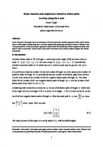
3.1 Rook placements and involutions Given a rook placement R of half-perimeter n, we define an involution α(R) by the following construction: label the north-east boundary of R with integers from 1 to n. This implies that each column or row has a label between 1 and n. If a column, or row, is labelled by i and does not contain a rook, it is a fixed point of α(R). Also, if there is a rook at the intersection of column i and row j, then α(R) sends i to j (and j to i). Given a rook placement R of half-perimeter n, we also define a Young diagram β(R) by the following construction: if we remove all rows and columns of R containing a rook, the remaining cells form a Young diagram, which we denote by β(R). We also define φ(R) = (α(R), β(R)). See Figure 1 for an example. ×× ◦ ××× ◦× R= ◦ × × ×

φ(R) =

b b b b b b b b b b,

!

Fig. 1: Example of a rook placement and its image by the map φ.

Proposition 7 The map φ is a bijection between rooks placements in Young diagrams of half-perimeter n, and ordered pairs (I, λ) where I is an involution on {1, . . . , n} and λ a Young diagram of half-perimeter |Fix(I)|. If φ(R) = (I, λ), the number of crosses in R is the sum of |λ| and some parameter µ(I). Proof: This kind of bijection rather classical, see for instance [4, 13]. Note that the pairs (I, λ) may be seen as involutions on {1, . . . , n} with a weight 2 on each fixed point. For the second part of the proposition, we just have to distinguish different kinds of crosses in the rook placement R. For example, the crosses with no rook in the same line and column are enumerated by |λ|. 2 Corollary 2 Let Tj,k,n be the sum of weights of rook placements of half perimeter n, with k lines and j lines without rooks. Then for any j,k,n, we have: n − 2k + 2j Tj,k,n = y j T0,k−j,n . (6) j q Proof: The previous proposition means that the number of crosses is an additive parameter with respect to the decomposition R 7→ (I, λ). This naturally lead to a factorisation of the generating function. 2


45

3.2 The recurrence Proposition 8 We have the following recurrence relation: T0,k,n = T0,k,n−1 + py[n + 1 − 2k]q T0,k−1,n−1 .

(7)

Proof: We have the relation: T0,k,n = T0,k,n−1 + pT1,k,n−1 .

(8)

Indeed, we can distinguish two cases, whether a rook placement enumerated by T0,k,n has a rook in its first column or not. These two cases give respectively the two terms of the previous identity. To end the proof we can apply identity (6) to the second term. 2 The recurrence (7) is solved by the following formula. Proposition 9 T0,k,n = q

−2k

k X n − 2k + i n n i i(i+1) 2 − . (−1) q i k−i k−i−1 q i=0

(9)

From this proposition, identity (6), and a q-binomial identity, we derive a formula for Tj,k,n . Proposition 10 k X j=0

Tj,k,n =

k X n j

j=0

−

n j−1

q(k+1−j)(n−k−j) −q(k−j)(n−k−j) +q(k−j)(n+1−k−j) −q(k+1−j)(n+1−k−j) (1−q)qn

.

Summing this identity over k gives the following result. Proposition 11 ˆ + E)|V ˆ hW |(y D i = (1 + y)G(n) − G(n + 1), ⌊n 2⌋

where

G(n) =

X n j=0

j

(10)

n−2j X n y i+j−1 q i(n+1−2j−i) . − j−1 i=0

Pk This formula is a linear combination of the polynomials Pk = i=0 y i q i(k+1−i) , the coefficients being polynomials in y, just as in Theorem 1. With this result and the inversion formula (4), we can prove Theorem 1: the last step is a simple binomial simplification.

4 Applications Among all the objects of the list in Proposition 1, the most studied are probably permutations and the pattern 13-2, see for example [5, 7, 18, 19]. In particular, in [5, 19] we can find methods for obtaining, as a function of n for a given k, the number of permutations of size n with exactly k occurrences of pattern 13-2. By taking the Taylor series of (1), we obtain direct and quick proofs for these results. As an illustration we give the formulae for k ≤ 3 in the following proposition.

46


Proposition 12 The order 3 Taylor series of hW |(D + E)n−1 |V i is: (n + 1)(n + 2) 2n n 2n 2n 2 n−1 q + q 3 + O(q 4 ), hW |(D + E) |V i = Cn + q+ 2 n−4 6 n−5 n−3 where Cn is the nth Catalan number. More generally, a computer algebra system can provide higher order terms, for example it takes no more than a few seconds to obtain the following closed formula for [q 10 ]hW |(D + E)n−1 |V i: (2n)! 13 + 70 n12 + 2093 n11 + 32354 n10 + 228543 n9 − 318990 n8 10!(n+12)!(n−8)! n −17493961 n7 − 104051458 n6 − 6828164 n5 + 2022876520 n4 +6310831968 n3 + 5832578304 n2 + 14397419520 n + 5748019200 ,

which is quite an improvement compared to the methods of [19]. In addition to exact formula, we can give asymptotic estimates, for example for the number of permutations with a given number of occurrences of pattern 13-2. Theorem 2 For any fixed m ≥ 0, 3

4n nm− 2 [q m ]hW |(D + E)n−1 |V i ∼ √ πm!

as n → ∞.

2n 2n 2n 1 Proof: When n → ∞, the numbers n−k − n−k−2 are dominated by the Catalan number n+1 n . This implies that in (1 − q)n hW |(D + E)n−1 |V i, each higher order term grows at most as fast as the constant term Cn . On the other side, the coefficient of q m in (1 − q)−n is asymptotically nm /m!. 2 Since any occurrence of the pattern 13-2 in a permutation is also an occurrence of the pattern 1-3-2, a permutation with k occurrences of the pattern 1-3-2 has at most k occurrences of the pattern 13-2. So we get the following corollary. Corollary 3 Let ψk (n) be the number of permutations in Sn with at most k occurrences of the pattern 1-3-2. For any constant C > 1 and k ≥ 0, we have 3

4n nk− 2 ψk (n) ≤ C √ πk! when n is sufficiently large. So far we have only used Corollary 1. Now we illustrate what can be done with the refined formula given in Theorem1. For example, when q = 0 then the coefficient of y m is given by the expres n Pn n n n sion k=0 (−1)k m . This is equal to the Narayana number N (n, m) = m+k − m−1 m+k+1 n 1 n n m m−1 (see [27] for a combinatorial proof). We can also get the coefficients for higher powers of q. For it is conjectured in [27] that the example n n coefficient of qy m in hW |y(yD + E)n−1 |V i is equal to m+1 . Applying our results we can prove: m−2


47

Proposition 13 The coefficients of qy m and q 2 y m in hW |y(yD + E)n−1 |V i are respectively: n n n+1 n + 1 nm + m − m2 − 4 . and 2(n + 1) m+1 m−2 m−2 m+2 Proof: A naive expansion of the Taylor series in q gives a lengthy formula, which is simplified easily after n 2 noticing that it is the product of m and a rational fraction of n and m. 2

Acknowledgements The authors want to thank Lauren Williams for her interesting discussions and suggestions.

References [1] R. A. Blythe, M. R. Evans, F. Colaiori and F. H. L. Essler, Exact solution of a partially asymmetric exclusion model using a deformed oscillator algebra, J. Phys. A: Math. Gen. Vol. 33, (2000), 23132332. [2] R. Brak, S. Corteel, J. Essam, R. Parviainen and A. Rechnitzer, A combinatorial derivation of the PASEP stationary state. Electron. J. Combin. 13 (2006), no. 1, 108, 23 pp. [3] R. Brak, and J.W. Essam, Asymmetric exclusion model and weighted lattice paths. J. Phys. A 37 (2004), no. 14, 4183–4217. [4] A. Burstein, On some properties of permutation tableaux, Ann. Combin. 11(3-4), (2007), 355-368. [5] A. Claesson, T. Mansour, Counting Occurrences of a Pattern of Type (1,2) or (2,1) in Permutations, Adv. in App. Maths. 29, (2002), 293-310. [6] S. Corteel, Crossings and alignments of permutations, Adv. in App. Maths. 38(2), (2007), 149-163. [7] S. Corteel and P. Nadeau, Bijections for permutation tableaux, Eur. Jour. of Comb 30(1), (2009), 295-310. [8] S. Corteel and L. K. Williams, Tableaux combinatorics for the asymmetric exclusion process, Adv. in App. Maths. 39(3), (2007), 293-310. [9] B. Derrida, M. Evans, V. Hakim, V. Pasquier, Exact solution of a 1D asymmetric exclusion model using a matrix formulation, J. Phys. A: Math. Gen. 26 (1993), 1493-1517. [10] A. Garsia and J. Remmel, q-Counting rook configurations and a formula of Frobenius. J. Combin. Theory, Ser. A 41, (1986), 246-275. [11] M. Josuat-Vergès, Rook placements in Young diagrams and permutation enumeration, submitted (2008). arXiv:0811.0524 [12] A. Kasraoui, D. Stanton, J. Zeng, The combinatorics of Al-Salam-Chihara q-Laguerre polynomials, preprint (2008). arXiv:0810.3232v1.

48


[13] S. Kerov, Rooks on Ferrers Boards and Matrix Integrals, Zapiski. Nauchn. Semin. POMI, v.240 (1997), 136-146. [14] J.C. Novelli, J-Y. Thibon and L.K. Williams, Combinatorial Hopf algebras, noncommutative HallLittlewood functions, and permutation tableaux, preprint (2008). arXiv:0804.0995 [15] A. Postnikov, Total positivity, arxiv:math.CO/0609764.

Grassmannians,

and

networks,

Preprint

(2006).

[16] T. Prellberg and R. Brak, Critical Exponents from Non-Linear Functional Equations for Partially Directed Cluster Models, J. Stat. Phys., Vol. 78 (1995), 701-730. [17] R. P. Stanley, Enumerative combinatorics Vol. 1, Cambridge university press (1986). [18] E. Steingr´ımsson, L. K. Williams, Permutation tableaux and permutation patterns, J. Combin. Theory Ser. A, Vol. 114(2), (2007), 211-234. [19] R. Parviainen, Lattice path enumeration of permutations with k occurrences of the pattern 2-13, Journal of Integer Sequences, Vol. 9 (2006), Article 06.3.2. [20] J.-G. Penaud, A bijective proof of a Touchard-Riordan formula, Disc. Math., Vol. 139 (1995), 347360. [21] M. Rubey, Nestings of Matchings and Permutations and North Steps in PDSAWs, FPSAC2008 (2008). arXiv:0712.2804 [22] J. Touchard, Sur un problème de configurations et sur les fractions continues, Can. Jour. Math., Vol. 4 (1952), 2-25. [23] M. Uchiyama, T. Sasamoto, M. Wadati, Asymmetric simple exclusion process with open boundaries and Askey-Wilson polynomials, J. Phys. A: Math. Gen. 37 (2004), 4985-5002. [24] A. Varvak, Rook numbers and the normal ordering problem, J. Combin. Theory Ser. A, Vol. 112(2), (2005), 292-307. [25] X.G. Viennot, Alternative tableaux and permutations, in preparation (2008). [26] X.G. Viennot, Alternative tableaux and partially asymmetric exclusion process, in preparation (2008). [27] L. K. Williams, Enumeration of totally positive Grassmann cells, Adv. Math., Vol. 190(2), (2005), 319-342.