Measuring Network Security Using Dynamic Bayesian
Network
Marcel Frigault and Lingyu Wang Concordia Institute for Information Systems Engineering Concordia University Montreal, QC H3G 1M8, Canada
Anoop Singhal
Sushil Jajodia
Computer Security Division National Institute of Standards and Technology Gaithersburg, MD 20899, USA
Center for Secure Information Systems George Mason University Fairfax, VA 22030-4444, USA
[email protected]
[email protected]
{m_frig,wang}@encs.concordia.ca ABSTRACT Given the increasing dependence of our societies on networked in formation systems, the overall security of these systems should be measured and improved. Existing security metrics have generally focused on measuring individual vulnerabilities without consider ing their combined effects. Our previous work tackle this issue by exploring the causal relationships between vulnerabilities encoded in an attack graph. However, the evolving nature of vulnerabilities and networks has largely been ignored. In this paper, we propose a Dynamic Bayesian Networks (DBNs)-based model to incorpo rate temporal factors, such as the availability of exploit codes or patches. Starting from the model, we study two concrete cases to demonstrate the potential applications. This novel model provides a theoretical foundation and a practical framework for continuously measuring network security in a dynamic environment.
Categories and Subject Descriptors D.4.6 [Security and Protection]: Invasive software (e.g., viruses, worms, Trojan horses); K.6.5 [Security and Protection]: Unau thorized access (e.g., hacking, phreaking)
General Terms Security
1.
INTRODUCTION
Our society has become increasingly dependant on the reliabil ity and proper functioning of a vast number of interconnected in formation systems. To improve the security of these systems, it is necessary to measure the amount of security provided by differ ent configurations since you cannot improve what you cannot mea sure [12]. The aim of our research is to develop coherent, logical and applicable security metrics for computer networks.
Permission to make digital or hard copies of all or part of this work for personal or classroom use is granted without fee provided that copies are not made or distributed for profit or commercial advantage and that copies bear this notice and the full citation on the first page. To copy otherwise, to republish, to post on servers or to redistribute to lists, requires prior specific permission and/or a fee. QoP’08, October 27, 2008, Alexandria, Virginia, USA. Copyright 2008 ACM 978-1-60558-321-1/08/10 ...$5.00.
There exist considerable research and standard techniques for measuring individual vulnerabilities, such as the Common Vulner ability Scoring System (CVSS) [7]. However, by considering vul nerabilities on an individual basis, a network security administra tor could be misled in a situation where individual vulnerabilities scores are low but these vulnerabilities can be combined to com promise a critical resource. Our previous research explores the causal relationships between vulnerabilities encoded in an attack graph to model the overall security of a network, which includes a general framework [26], a real-valued metric [28], a probabilistic metric [24], and a Bayesian Network (BN)-based approach [8].
Problem Statement and Success Criteria. The main problem solved in this paper is the following. The evolving nature of vulnerabilities has largely been ignored in most existing work on network security metrics. The main hypothesis is that the threat posed by a vulnerability may change over time in to day’s dynamic network environment. When more technical details of a vulnerability become available, its exploitability or severity may need to be adjusted; when patches are released by vendors to counter an exploit, the vulnerability may become less severe; on the other hand, when exploit codes become more widely spread, the severity of a vulnerability may increase. Therefore, it is insuf ficient to rate vulnerabilities with fixed scores. In our understanding, a successful solution to network security metrics should meet following criteria. First, it should model var ious temporal aspects of a vulnerability. The temporal scores in CVSS [7] provide a partial solution. Second, the solution should combine the temporal scores of individual vulnerabilities into a global rating of security of the whole network at any given time. CVSS lacks such a capability as it does not take into considera tion the interplay of vulnerabilities in a given network. Third, it is also desirable that temporal trends and patterns can be discovered and used for reasoning about future security scores based on past incidents or observations. In this paper, we propose a Dynamic Bayesian Network (DBN) based model to incorporate relevant temporal factors, such as the availability of exploit codes or patches, into attack graph-based se curity metrics. As we shall show, our model meets all aforemen tioned success criteria of a network security metric. More specif ically, we first show how to interpret an attack graph as a special DBN; we then combine individual base scores of CVSS using their causal relationships; finally, we integrate the effect of temporal
scores of CVSS to derive the final measurement of security. To demonstrate potential applications of our model, we discuss two concrete cases where either the exploitability or the temporal score of a vulnerability is unobservable and can be derived through rea soning with the proposed model. The main contribution of the paper is two fold. First, by mod eling attack graphs as special DBNs, we devise a sound theoretic foundation for the development and application of security metrics in a dynamic environment. Second, by binding our model to the CVSS standard, we provide a practical way for deriving actionable knowledge about the overall security of a network. The rest of the paper is organized as follows. Section 2 reviews relevant concepts of attack graph and DBN. Section 3 describes the proposed model and discusses two concrete cases. Section 4 studies two cases of applying the model. Section 5 reviews related work. Section 6 discusses future work and concludes the paper.
2.
PRELIMINARIES
To be self-contained, this section reviews relevant concepts of the attack graph model and DBN.
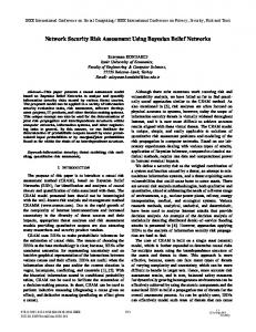
2.1 Attack Graph Model Attack graphs model the knowledge about how multiple vulner abilities may be combined for an attack. The model represents sys tem states using security-related conditions, such as the existence of vulnerabilities on a host or the connectivity between hosts, and state transitions using exploits of vulnerabilities. For our purposes, an attack graph is a directed graph with conditions and exploits as vertices, and their relationships as edges [1]. Figure 1 shows a toy example of network configuration on the left-hand side and the cor responding attack graph on the right-hand side. user(0) ftp_rhosts(0,1) host 0
trust(0,1) sshd_bof(0,1)
rsh(0,1) firewall
host 1
host 2
ftp
rsh
ssh
ftp rsh
user(1) ftp_rhosts(0,2)
ftp_rhosts(1,2)
trust(0,2)
trust(1,2)
rsh(0,2)
rsh(1,2) user(2) local_bof(2,2)
root(2)
Figure 1: Network Configuration and Attack Graph
Figure 1 depicts a simple scenario where a file server (host 1) of fers the File Transfer Protocol (ftp), secure shell (ssh), and remote shell (rsh) services; a database server (host 2) offers ftp and rsh ser vices. The firewall only allows ftp, ssh, and rsh traffic from a user workstation (host 0) to both servers. In the attack graph, exploits of vulnerabilities are depicted as predicates in ovals and conditions as predicates in clear texts. The two numbers inside parentheses denote the source and destination host, respectively. The attack
graph represents three self-explanatory sequences of attacks (at tack paths). For example, the right path is: sshd_bof (0, 1) → f tp_rhosts(1, 2) → rsh(1, 2) → local_bof (2).
2.2
Dynamic Bayesian Network
BNs offer a compact means to encode the entire range of condi tional relationships, which is particularly suitable for representing security metrics based on attack graphs. In [24], we calculate a probability value for each vertex to represent the likelihood of an average attacker reaching that vertex. A major assumption here is that exploits of different vulnerabilities are independent unless those exploits are related in the attack graph, which is not always true. For example, exploits of the same vulnerability may become easier on subsequent attempts, even though those exploits are not directly related in an attack graph [26]. Our recent BN-based attack graph approach eliminates this limitation by encoding such depen dencies among exploits as conditional probabilities in a BN [8]. It is also important to distinguish our BN-based attack graph from that by Liu et al. [13]. The key difference lies in that our approach assigns probabilities to exploits while their model assigns probabil ities to edges. Our approach is more practical in the sense that our vertex probability assignment is based on widely available standard measures, such as CVSS, whereas the edge probability assignment has little solid ground in [13]. In contrast to BN, Dynamic Bayesian Network (DBN) is a graph ical model for probabilistic inferences in dynamic domains that can enable users to monitor and update the system as time proceeds, and even predict further behaviors of the system [16]. Today’s net works are certainly dynamic environments, and the security of such an environment involves many temporal factors, such as the avail ability of exploit codes, the availability of patches or fixes, the con fidence in reported vulnerabilities, and so on. To incorporate such temporal factors in measuring network security, we extend our pre vious BN-based model to DBNs. In a typical DBN model, the system is represented as a sequence of BNs. Each BN represents a time slice of the DBN corresponding to a particular instant of time. As with the BN, arcs exists between the vertices within each time slice. In addition, the DBN will have arcs between certain vertices of successive time slices. In a DBN model, it can be assumed that the Markovian property is satisfied which implies that the state of the system depends only on the previous state. In addition, it is as sumed that the conditional dependencies among the vertices across the time slices are the same. Therefore, the system can be modeled with only 2 time slices (more strictly speaking, the first 1.5 slices). In DBNs, the vertices can be classified as either observable or un observable. The value of observable vertices are known a prior during the analysis process, whereas that of unobservable are not available but can be inferred. In order to provide the required links between the time slices, arcs can be introduced between a set of unobservable vertices and the necessary CPDs can be developed to encode the relationships existing between successive time slices.
3.
THE MODEL
This section introduces the proposed models in three steps. We first describe the value assignment for individual exploits based on CVSS scores; we then describe the model for static domain; finally, we discuss the models for dynamic domain in two cases.
3.1
CVSS-Based Individual Value Assignment
There are two inputs to our model, namely, attack graph and CVSS scores. First, we assume the attack graph of a given net work can be obtained using existing tools, such as the Topological Vulnerability Analysis (TVA) system, which can generate attack
graphs for more than 37,000 vulnerabilities taken from 24 infor mation sources including X-Force, Bugtraq, CVE, CERT, Nessus, and Snort [11]. Second, we assume the CVSS scores of vulnera bilities in the given attack graph can be obtained from existing vul nerability databases, such as the National Vulnerability Database (NVD) [18]. To facilitate further discussions, we review relevant CVSS concepts in the following. • The Base Score (BS) for each vulnerability quantifies its in trinsic and fundamental properties that are supposed to be constant over time and independent of user environments. The value of BS ranges from 0 to 10. • The Temporal Metric Values quantify a vulnerability when considering properties of the vulnerability that may change over time. The three temporal metric values used in CVSS are Exploitability (E), Remediation Level (RL), and Report Confidence (RC). In particular, the Exploitability (E) can take one of the four annotated values: 0.85 (U), 0.9 (PoC), 0.95 (F), and 1.00 (H). • For convenience, we name the product T GS = (E × RL × RC) as the Temporal Group Score (TGS). Based on the pos sible values of E, RL and RC [7], the value of TGS ranges from 0.67 to 1.0. • The Temporal Score (TS) is the product of BS and TGS: T S = round_to_1_decimal(BS × T GS)
3.2
We are now ready to use Bayesian network(BN) to represent at tack graph-based probabilistic metrics in the static case. The ver tices of the BN represent exploits derived from the attack graph. Each vertex is annotated with a probability assigned according to Equation 2. The CPD tables can then be developed to encode the probability values for each vertex and its conditional dependencies. Such a BN-based model allows propagating probabilities of an at tacker reaching each condition. In particular, we are interested in the goal state (the final conditions), which can be used as an indi cator about the overall security of the network. More formally, given an attack graph G(E ∪ C, Rr ∪ Ri ), we represent the attack graph using a Bayesian network which is a pair B = (G, Q) where G is the directed graph corresponding to the attack graph but with a different semantics, that is, the vertices rep resent the binary variables of the system and the edges represent the conditional relationships among the variables. Q is the set of parameters that quantify the BN such as the conditional distribu tion values for each variable (vertex). The joint distribution for a Bayesian network is represented in the standard � way as (the nota tions are self-explanatory): P (X1 ...Xn ) = n i=1 P (Xi |parents(Xi )). The unique aspect of this BN representation is the following. In an attack graph, the causal relationships between exploits can be disjunctive or conjunctive based on how they are related through conditions [8]. Such relationships are represented in our BN rep resentation using conditional probabilities of 0 or 1. More specifi cally, • We say a disjunctive relationship exists between any exploits e1 , e2 , . . . , en with respect to en+1 when ej Ri c holds for all j = 1, 2, . . . , n and some condition c, and cRr en+1 is true. In such a case, the probability assignment based on Equation 2 will satisfy P (en+1 = T |X) = 1 for all X that has ej = T hold for at least one j ∈ [1, n].
(1)
TS ranges from 0 to 10. We convert CVSS scores of a vulnerability to probabilities as follows. First, we convert the score BS (or TS in the dynamic case) to a probability using a simple approach of diving it by the do main size 10. We then associate this probability to all the exploits that has this vulnerability (recall that an exploit is a vulnerability bound to specific source and destination hosts). Second, CVSS scores are proposed for quantifying individual vulnerabilities only. Those scores ignore the causal relationships between exploits in the context of a given network, which is modeled in attack graphs. Therefore, we define the probability converted from a score as the conditional probability of an exploit when all of its preconditions in the attack graph are already satisfied (by other exploits that imply those conditions). More formally, consider an attack graph G as a directed graph G(E ∪ C, Rr ∪ Ri ) where E is a set of exploits, C a set of condi tions, and Rr ⊆ C × E and Ri ⊆ E × C are two relations. We regard each exploit as a binary variable that can take discrete values of T (True), which signifies the exploit has been successfully per formed by the attacker, or F (False) indicating the converse. Given any exploit e ∈ E, and its corresponding score BS (or T S in the dynamic case), we assign conditional probabilities as follows: P (e = T |∀c ∈ Rr (e) c = T ) = BS/10
(2)
For example, in Figure 1, we have P (rsh(0, 1) = T |trust(0, 1) = T ) = BSrsh(0,1) /10. Since the condition trust(0, 1) can only be satisfied by one exploit f tp_rhosts(0, 1), we can relate probabil ities of the two exploits as P (rsh(0, 1) = T |trust(0, 1) = T ) = P (rsh(0, 1) = T |f tp_rhosts(0, 1) = T ) = BSrsh(0,1) /10.
Static Domain
• We say a conjunctive relationship exists between exploits e1 , e2 , . . . , en with respect to en+1 when ej Ri cj and cj Rr en+1 both hold for all j = 1, 2, . . . , n and some conditions cj ’s. In such a case, we have P (en+1 = T |X) = 0 whenever X has ej = F hold for at least one j ∈ [1, n]. For example, Figure 2 shows a BN with three exploits A, B, and C in which an attacker can achieve the goal state by following one of either two paths (for simplicity, we shall omit conditions from now on). The probabilities are converted from BS scores (by dividing them by 10). Using Equation 2, we can construct the CPDs for each vertex as shown on the right-hand side of Figure 2. From the CPD tables, we can observe that C is true as long as at least one of A and B is true. This indicates a disjunctive relationship between A and B with respect to C. .3
.3 A
B
C .4
A
B
C
T
F
T
F
A
B
T
.3
.7
.3
.7
F
F
0
F 1
F
T
.4
.6
T
F
.4
.6
T
T
.4
.6
Goal State
Figure 2: Representing Attack Graphs as BNs The CPDs allow us to calculate the joint probability function for any exploit or condition in the given network. In this case,
we are interested in the probability that C = T (that is, vulnera bility C has been successfully exploited). This can be calculated � as P (C = T ) = A,B∈{T,F } P (C = T, A, B) = 0.204. As an example application, this calculation can be applied to different network configurations in order to compare their relative security.
3.3 Dynamic Domain As described in Section 3.1, CVSS provides several temporal scores in addition to base scores in order to model the time variant factors in determining the severity of a vulnerability. Such scores are, however, still intended for individual vulnerabilities instead of the overall security of a network. Our objective is to evolve the aforementioned BN-based model to DBNs such that we can model the security of dynamically changing networks. The temporal links between time slices of the DBN will be established between the unobservable variables of the model. Those links will then enable the inference of unknown values based on the previous slice of the DBN. We introduce two additional sets of vertices into the previous BN model. The first is the collection of BS vertices that corre spond to the base score of vulnerabilities. The second is the collec tion of TGS vertices that correspond to the temporal group scores as defined in Section 3.1. The existing exploit vertices will then carry the final metric score TS (instead of the BS in the static case), which has a similar role as the calculated scores in the case of static domain (as described in Section 3.2). However, in the static do main, the final score is calculated based on the base score and the causal relationship between this exploit and others, whereas in the dynamic domain, the final score of each exploit will depend on four factors: The base score, the temporal score, the causal relationship between exploits and others, and the previous time slice (this will become clearer later when we discuss the two concrete cases). Formally, given an attack graph G as a directed graph G(E ∪ C, Rr ∪ Ri ), we define EBS and ET GS with the same cardinality as E to represent the set of BS and TGS nodes. We then obtain an enriched set of nodes as E ' = E ∪ EBS ∪ ET GS . Let G' be the directed graph corresponding to E ' in which the relations Rr and Ri remain the same. Then we can have the one slice BN as a pair (G' , Q) where Q represents the conditional probabilities assigned as before. We then define a DBN as a pair (B0 , Bd ), where B0 defines the prior P (X1 ), and Bd is a two-slice temporal Bayes net(2TBN) that defines P (Xt |Xt−1 ) by means of a DAG: � i i P (Xt |Xt−1 ) = N i=1 P (Xt |parents(Xt )). For B0 , conditional probabilities are assigned in a similar way as in the static case except that now we use the TS scores instead of the BS scores. More specifically, the TS scores are derived as the product of BS and TGS using Equation 1. The derived TS scores are then assigned as conditional probabilities based on Equation 2. For Bd , the assignment of interslice conditional probabilities will depend on specific needs of applications, since different variables in a time slice may be regarded as unobservable, and the effect of a previous slice will depend on the semantics of the variables in question. To make our discussions more concrete, we shall discuss two cases to illustrate the potential of our model. First, the TS score of each vulnerability is of interest (for exam ple, to security administrators of a network) and needs to be derived from the base scores, temporal scores, and interslice dependency. More formally, our DBN (B0 , Bd ) will be a two-slice temporal Bayes net(2TBN) that defines a DAG including only arcs between nodes in E. In this case, we assign conditional probabilities as fol lows. When a vulnerability has been successfully exploited in one time slice, then its probability of being exploited in the next time slice is equal to “1”, otherwise the probability assigned to the ex
ploit vertex is the same as in the case of B0 (that is, the previous slice has no effect). This simple choice reflects the intuition that a successful exploit will lead to more exploits of the same vulnera bility (more realistic ways for assigning such probabilities certainly exist). Second, the temporal score of a vulnerability is of interest (for example, to security vendors who maintain those scores) and needs to be derived from base scores and the observed TS scores (esti mated from the amount of reported security incidents involving that vulnerability). More formally, in this case, our DBN (B0 , Bd ) will be a two-slice temporal Bayes net(2TBN) that defines a DAG in cluding only arcs between nodes in T GS (or its components). For this case, the conditional probabilities can be assigned to reflect the temporal trends in those scores. In next section, we shall rely on a simple choice that if the E (Exploitability) score is confirmed to be one of the four discrete levels (U=0.85, PoC=0.9, F=0.95, or H=1.0 [7]), then its calculated value will be rounded to the same level in the next slice. For example, if without considering interslice conditional probabilities we can calculate E as 0.94, then the conditional probability that E is rounded to PoC (instead of F) given E=PoC in the preceding slice will be assigned as 1 (again, this is only an illustrative example and other temporal trends can certainly be used here).
4.
CASE STUDY This section studies two examples of applying the proposed model.
4.1
Case 1: Exploit Scores Are Unobservable
To security administrators, the final score of each exploit is usu ally unobservable, whereas the BS and TGS vertices are observ able. The observable values for the BS vertices can be obtained from NVD and the observable values for the TGS vertices can be calculated using CVSS equations described in section 3.1. To model the temporal dependency between time slices, arcs linking the time slices are introduced between the exploit vertices since they are unobservable. Our objective is to infer their values and eventually calculate the likelihood of attackers in reaching the goal state. Figure 3 shows our DBN model in this case through a toy ex ample of two exploits. In our model, we define the exploit vertices (“addusrphp” and “sunvect” in this example) to be conditionally dependant on their respective BS and TGS vertex values as repre sented graphically in Figure 3. In the example, the value of ex ploit “sunvect” is conditionally dependant on the value of exploit vertex “addusrphp”. This causal relationship implies that vulnera bility “addusrphp” must be exploited first in order for vulnerability “sunvect” to be exploited. In this example, the goal state is the successful exploitation of vulnerability “sunvect”. To model the temporal dependency, arcs linking the time slices are introduced between “addusrphp” and “sunvect”. To complete the model, we need to develop the CPDs for the intraslice rela tionships (within the same time slice) and the interslice relation ships (from one time slice to the next). Suppose our objective is to calculate the probability value of an attacker successfully ex ploiting “sunvect” for any time slice. From NVD we obtain the BS for each vulnerability as follows: BS(addusrphp) = 7.5 and BS(sunvect) = 10.0. For simplicity, we will consider only the E temporal metric and will assume initially the E metric is Unproven (U). We compute T GS = 0.85 ∗ 1.0 ∗ 1.0. We can then derive the probability for “addusrphp” as 0.64 and that for “sunvect” as 0.85. Figure 4 illustrates the intraslice CPDs. We can then compute that P (sunvect = T ) = 0.54 for the first slice. Figure 5 illustrates how the interslice CPD can be calculated for later slices (in this
addusrphpi
addusrphp1
addusrphp0
addusrphpn
BS1
BS0
TGS0
1
0
F
(BSaddusrphp*TGSaddusrphp)/10
1-(BSaddusrphp*TGSaddusrphp)/10
TGSn
sunvectn
BS1
F
sunvecti
sunvect1
EB0
T
T
BSn
TGS1
sunvect0
addusrphpi-1
sunvecti-1
T
T
1
F 0
F
(BSsunvect*TGSsunvect)/10
1-(BSsunvect*TGSsunvect)/10
BSn
Figure 5: Interslice CPDs TGS1
BBase0
Time 0
TGSn
Time 1
Time n
Figure 3: DBN Model for the First Case
particular example the values do not change in the 2nd slice so we omit the table).
based on the DBN model. Figure 6 illustrates the DBN model for this case where only the unobservable E metric vertices are linked from one time slice to the next. The interpretation is that the value of the E metric in the previous time slice will have an impact on determining the likelihood of which state the E metric vertex will be in during the subsequent time slices. Figure 7 shows the intraslice CPDs while Figure 8 shows the interslice CPDs (we only show the results since the calculation is similar to the previous case).
addusrphp T
F
(BSaddusrphp*TGSaddusrphp)/10
1-(BSaddusrphp*TGSaddusrphp)/10
BS0
sunvect A
T
T
T
(BSsunvect*TGSsunvect)/10
1-(BSsunvect*TGSsunvect)/10
F
0
1
addusrphp
addusrphp0
BS1
addusrphp1
BSn
TGS0
TGS1
TGSn
E0
E1
En
BS0
sunvect0
BS1
sunvect1
addusrphpn
BSn sunvectn
T
F
0.64
0.36
TGS0
TGS1
TGSn
E0
E1
En
sunvect A
T
T
T
0.85
0.15
F
0
1
Time 0
To vendors that create and maintain the CVSS databases, tempo ral scores are unobservable and must be estimated from base scores and reported security incidents. We now consider the case where the Exploitability (E) temporal metric vertices for each vulnerabil ity are unobservable. In the previous case, we were able to observe the E metric value and then compute the TGS value. In this case, we have the reverse situation. The goal in this case is to update the E Temporal Metric values for maintaining the CVSS databases
Time n
Figure 6: DBN Model for Case 2
Figure 4: Intraslice CPDs
4.2 Case 2: Temporal Scores Are Unobserv able
Time 1
We now discuss an example analysis using the model. Suppose reported security incidents show that the likelihood that “addusr php” will be exploited in “Time 0” is 0.66 and that the likelihood of “sunvect” being exploited is 0.94. We can calculate the TGS vertex scores for each exploit as 0.66/0.75 = 0.88 and 0.94/1 = 0.94, respectively. We then need to map these calculated scores to one of the four discrete levels given by CVSS (U=0.85, POC=0.9, F=0.95 and H=1.0). The DBN model will allow us to base such a map ping on the previous slice, since a previously confirmed level will support mapping the calculated value to the same level.
5.
RELATED WORK
P(E0=column value|TGS0)
TGSi Round to {0.85, 0.9, 0.95,1.0) U
POC
F
0.85
1.0
0
0
H 0
0.9
0
1.0
0
0
0.95
0
0
1.0
0
1.0
0
0
0
1.0
Figure 7: Intraslice CPDs
P(Ei=column value|Ei-1)
Ei-1
TGSi Round to {0.85, 0.9, 0.95,1.0) U
POC
F
H
U
0.85
1.0
0
0
0
0.9
.3
.7
0
0
0.95
0
.3
.7
0
1.0
0
0
0
1.0
0.85
1.0
0
0
0
0.9
0
1.0
0
0
0.95
0
.3
.7
0
1.0
0
0
0
1.0
0.85
1.0
0
0
0
0.9
0
1.0
0
0
0.95
0
0
1.0
0
POC
F
H
1.0
0
0
0
1.0
0.85
1.0
0
0
0
0.9
0
1.0
0
0
0.95
0
0
1.0
0
1.0
0
0
0
1.0
Figure 8: Interslice CPDs
The idea of using BNs to model network vulnerabilities and de termine a quantitative value representing the security of a network has been explored by Liu and Man [13]. A BN is used to model all potential atomic attack steps in a network. Each vertex represents a single security property violation state and each edge corresponds to an exploitation of one or more exhibited vulnerabilities. They assign edge weights to represent the probability of successful ex ploits. The difference between their work and ours is detailed in Section 3. Our application of DBN is inspired by the work by An et al. [2] for privacy intrusion detection. They employ DBN to re late a database operator’s intention to observable factors, such as the time spent on a certain operation. The issue of security metrics has recently attracted much atten tion [4, 15]. The NIST’s efforts on standardizing security metrics are reflected in [17] and more recently in [23]. Another overview of many aspects of network security metrics is given in [10]. Based the exploitability concept, a qualitative measure of risk is given in [5]. Another approach measures the relative risk of different configurations using the weakest attacker model, that is the least conditions under which an attack is possible [19]. Yet another se ries of work measures how likely a software is vulnerable to at tacks using a metrics called attack surface [14]. These work allow a partial order to be established on different network configurations based on their relative security. However, the treatment of many aspects of security is still qualitative in nature. For example, the resources are still treated equally important (no explicit evaluation
of damages) and the resistance to attacks is regarded as binary (an attack is either impossible or trivial). Relevant work exist in other areas, such as the study of trust in distributed systems. Beth et al. proposed a metrics for measuring the trust in an identity that has been established through overlap ping chains of certificates [6]. The way they combine values of trust in certificates into an overall value of trust proves to be use ful in our study. Similarly, the design principles given by Reiter et al. are intended for developing metrics of trust, but we found these principles applicable to our study [20]. Structures similar to attack graphs are used for risk analysis in safety-critical systems although the focus is not on vulnerabilities but on trust relationships [3]. Our model, used as a monitoring system, shares similarity with the tech nique for testing whether a finite execution of events generated by a program violates a linear temporal logic (LTL) formula [9]. To generate attack graphs, topological vulnerability analysis enumer ates potential multi-step intrusions based on prior knowledge about vulnerabilities and their relationships [21, 22]. Wang et al. [26] proposed a framework for using combining functions to determine the combined effect of vulnerabilities in a network. They proposed the idea of using an analogy to the resis tance of electrical circuits in [27] and address the issue of additional dependency between exploits although the solution is not entirely satisfactory since cycles in attack graphs are largely ignored. Wang et al. also proposed a probabilistic network security metric based on attack graphs [24]. They propose the use of probability scores for each vulnerability to represent the likelihood that one attacker will exploit the vulnerability or the percentage of attackers that suc cessfully exploit the vulnerability. Our work adopt this same con cept but will use it to develop conditional probability tables for each exploit and then demonstrate how the use of DBNs can be used to determine network security. The work on minimum-cost network hardening represents an early effort toward the quantitative study of network security [25]. This work quantifies the cost of remov ing vulnerabilities in hardening a network, but it does not consider other hardening options, such as modifying the connectivity. It also has the limitation of adopting a qualitative view of damages (that is, all the given critical resources are equally important) and of attack resistance (that is, attacks on critical resources are either impossible or trivial).
6.
CONCLUSION AND FUTURE WORK
This paper has pointed out the lack of consideration for temporal factors in previous work on measuring network security. This paper then proposes a novel DBN-based model for capturing the evolv ing nature of vulnerabilities in a computer network. We show that DBN can be derived from attack graphs and standard metric val ues and the derived model can be used for analyzing the constantly changing security aspects of a network. We develop our model in close association with the standard CVSS scores in order to ensure the model can lead to actionable knowledge. As future work, we are implementing a practical tool for measur ing network security by integrating attack graphs generated by the TVA system [11] with CVSS scores provided by NVD. Based on such a tool, we plan to conduct real-world experiments to evaluate our methods. We will continue to refine our approach using DBNs to encompass more properties of the temporal metrics established in the CVSS in order to develop a more accurate model. We will examine how the model can be refined to take into consideration the environmental factors of CVSS. We will also study the appli cation of the proposed model for hardening a vulnerable network with the least cost. In our model, we made the assumption that the Markovian Property applied. It would be interesting to explore the
usefulness of a model where this is not necessarily the case.
Acknowledgements The authors thank the anonymous reviewers and the shepherd Fabio Massacci for their valuable comments. This material is based upon work supported by National Institute of Standards and Technology Computer Security Division; by Homeland Security Advanced Re search Projects Agency under the contract FA8750-05-C-0212 ad ministered by the Air Force Research Laboratory/Rome; by Army Research Office under grant W911NF-05-1-0374, by Federal Avia tion Administration under the contract DTFAWA-04-P-00278/0001, by the National Science Foundation under grants CT-0627493, IIS 0242237 and IIS-0430402, by Natural Sciences and Engineering Research Council of Canada under Discovery Grant N01035, and by Fonds de recherche sur la nature et les technologies. Any opin ions, findings, and conclusions or recommendations expressed in this material are those of the authors and do not necessarily reflect the views of the sponsoring organizations.
7.
REFERENCES
[1] P. Ammann, D. Wijesekera, and S. Kaushik. Scalable, graph-based network vulnerability analysis. In Proceedings of the 9th ACM Conference on Computer and Communications Security (CCS’02), 2002. [2] X. An, D. Jutla, and N. Cercone. Privacy intrusion detection using dynamic bayesian networks. In Proceedings of the 8th International Conference for Electronic Commerce (ICEC’06), pages 208–215, 2006. [3] Y. Asnar, P. Giorgini, F. Massacci, and N. Zannone. From
trust to dependability through risk analysis. In Proceedings
of ARES’07, 2007.
[4] Applied Computer Security Associates. Workshop on. In
Information Security System Scoring and Ranking, 2001.
[5] P. Balzarotti, M. Monga, and S. Sicari. Assessing the risk of using vulnerable components. In Proceedings of the 2nd ACM workshop on Quality of protection, 2005. [6] T. Beth, M. Borcherding, and B. Klein. Valuation of trust in open networks. In Proceedings of the Third European Symposium on Research in Computer Security (ESORICS’94), pages 3–18, 1994. [7] Common vulnerability scoring system - SIG. available at:
http://www.first.org/cvss/, Accessed May 2008.
[8] M. Frigault and L. Wang. Measuring network security using bayesian network-based attack graphs. In Proceedings of the 3rd IEEE International Workshop on Security, Trust, and Privacy for Software Applications (STPSA’08), 2008. [9] Klaus Havelund and Grigore Roşu. Efficient monitoring of safety properties. Int. J. Softw. Tools Technol. Transf., 6(2):158–173, 2004. [10] K.S. Hoo. Metrics of network security. White Paper, 2004. [11] S. Jajodia, S. Noel, and B. O’Berry. Topological analysis of network attack vulnerability. In V. Kumar, J. Srivastava, and A. Lazarevic, editors, Managing Cyber Threats: Issues, Approaches and Challenges. Kluwer Academic Publisher, 2003. [12] A. Jaquith. Security Metrics Replacing Fear, Uncertainty, and Doubt. AddisonWesley, 2007. [13] Y. Liu and H. Man. Network vulnerability assessment using bayesian networks. In Proceedings of SPIE - Data Mining, Intrusion Detection, Information Assurance and Data Networks Security (SPIE’05), pages 61–71, 2005.
[14] K. Manadhata, J.M. Wing, M.A. Flynn, and M.A. McQueen. Measuring the attack surfaces of two ftp daemons. In Quality of Protection Workshop, 2006. [15] John McHugh. Quality of protection: Measuring the unmeasurable? In Proceedings of QoP (QoP’06), 2006. [16] V. Mihajlovic and M Petkovic. Dynamic bayesian networks: A state of the art. available at: http://doc.utwente.nl/36632/1/0000006a.pdf. [17] National Institute of Standards and Technology. Technology assessment: Methods for measuring the level of computer security. NIST Special Publication 500-133, 1985. [18] National vulnerability database. available at: http://www.nvd.org, May 9, 2008. [19] J. Pamula, S. Jajodia, P. Ammann, and V. Swarup. A weakest-adversary security metric for network configuration security analysis. In Proceedings of the 2nd ACM workshop on Quality of protection, pages 31–38, New York, NY, USA, 2006. ACM Press. [20] M.K. Reiter and S.G. Stubblebine. Authentication metric analysis and design. ACM Transactions on Information and System Security, 2(2):138–158, 5 1999. [21] R. Ritchey and P. Ammann. Using model checking to analyze network vulnerabilities. In Proceedings of the 2000 IEEE Symposium on Research on Security and Privacy (S&P’00), pages 156–165, 2000. [22] O. Sheyner, J. Haines, S. Jha, R. Lippmann, and J.M. Wing. Automated generation and analysis of attack graphs. In Proceedings of the 2002 IEEE Symposium on Security and Privacy (S&P’02), 2002. [23] M. Swanson, N. Bartol, J. Sabato, J. Hash, and L. Graffo. Security metrics guide for information technology systems. NIST Special Publication 800-55, 2003. [24] L. Wang, T. Islam, T. Long, A. Singhal, and S. Jajodia. An attack graph-based probabilistic security metric. In Proceedings of The 22nd Annual IFIP WG 11.3 Working Conference on Data and Applications Security (DBSEC’08), 2008. [25] L. Wang, S. Noel, and S. Jajodia. Minimum-cost network hardening using attack graphs. Computer Communications, 29(18):3812–3824, 11 2006. [26] L. Wang, A. Singhal, and S. Jajodia. Measuring network security using attack graphs. In Proceedings of the 3rd ACM workshop on Quality of protection (QoP’07), New York, NY, USA, 2007. ACM Press. [27] L. Wang, A. Singhal, and S. Jajodia. Measuring the overall security of network configurations using attack graphs. In Proceedings of 21th IFIP WG 11.3 Working Conference on Data and Applications Security (DBSEC’07), 2007. [28] L. Wang, C. Yao, A. Singhal, and S. Jajodia. Interactive analysis of attack graphs using relational queries. In Proceedings of 20th IFIP WG 11.3 Working Conference on Data and Applications Security (DBSEC’06), pages 119–132, 2006.