Mechanical Engineering Journal - Tohoku University

Bulletin of the JSME

Vol.4, No.2, 2017

Mechanical Engineering Journal Phase-field topology optimization model that removes the curvature effects Tomohiro TAKAKI* and Junji KATO** * Faculty of Mechanical Engineering, Kyoto Institute of Technology Matsugasaki, Sakyo, Kyoto 606-8585, Japan E-mail: [email protected] ** Mechanics of Materials Laboratory, Tohoku University 6-6, Aoba, Aramaki, Aoba, Sendai 980-8579, Japan

Received: 2 August 2016; Revised: 15 October 2016; Accepted: 7 February 2017

Abstract The conventional phase-field topology optimization (PFTO) models minimize not only the objective function but also the interface energy. In the present study, a new PFTO model, which minimizes only the objective function, is developed by removing the curvature effect from the conventional PFTO model. Simulations of elastic strain energy minimization under a constant-volume constraint condition of a cantilever are performed using the developed and conventional PFTO models. From the simulation results, we confirm that the developed PFTO model that removes the curvature effects can efficiently optimize only the objective function. Key words : Phase-field method, Finite element method, Topology optimization, Maximum stiffness, Curvature

1. Introduction The phase-field method has emerged as a powerful numerical tool to simulate the formation process of complicated material microstructures (Chen, 2002). The successful work of Kobayashi to simulate the complicated and beautiful dendrite growth during solidification opened the phase-field study area (Kobayashi, 1993; Kobayashi, 1994). Since then, in the solidification field (Asta et al., 2009; Steinbach, 2009; Takaki, 2014), the phase-field model has been applied to binary alloys (Warren and Boettinger, 1995; Wheeler et al., 1992), polycrystals (Miyoshi and Takaki, 2016; Steinbach and Pezzolla, 1999), quantitative models (Karma and Rappel, 1996; Ohno and Matsuura, 2009), multi-component alloys (Ohno et al., 2012), coupled models with convection (Beckermann et al., 1999; Rojas et al., 2015; Takaki et al., 2015b), and large-scale computations (Sakane et al., 2015; Shibuta et al., 2015; Takaki et al., 2014; Takaki et al., 2013; Yamanaka et al., 2011). The great success of the phase-field method in material science is due to the advantages of the phase-field method: tracking the interface position is not necessary, the curvature effects are included in the model, the evolution equations can be derived from the free-energy functional based on the second law of thermodynamics, the discretization of the time evolution equations is easy, and so on. Even with the exception of material microstructures, the phase-field method is widely used in surface morphology (Takaki et al., 2006; Takaki et al., 2008), dislocation dynamics (Wang and Li, 2010), crack propagation (Ambati et al., 2015; Oshima et al., 2014), biomechanics (Lee et al., 2016; Takaki et al., 2015a), multiphase flow (Takada et al., 2006), and so on. The phase-field method has also been successfully applied to the topology optimization problem. Here and in the rest of this paper, we call the topology optimization model using the phase-field method as the phase-field topology optimization (PFTO) model. To the best of our knowledge, the first application of the phase-field method to topology optimization was performed by Bourdin and Chambolle (Bourdin and Chambolle, 2003; Bourdin and Chambolle, 2006). For a while since then, the Cahn–Hilliard (CH) model has been widely applied to topology optimization (Burger and Stainko, 2006; Dedè et al., 2012; Wang and Zhou, 2004a; Wang and Zhou, 2004b; Zhou and Wang, 2007; Zhou and Wang, 2006). The CH model can conserve the volume without any operation. However, it needs a very small time increment because the time evolution equation becomes a fourth-order partial differential equation. The first successful application of the Allen–Cahn (AC) equation to topology optimization was performed by Takezawa et al. (Takezawa et al., 2010) in a minimum compliance problem. Because the model is very simple and therefore has wide versatility and applicability, it was employed in many subsequent studies. Choi et al. (Choi et al., 2011) enabled spontaneous nucleation of holes using a reaction–diffusion equation without a double-well potential in the phase-field model. Yamada et al. (Yamada et al., 2010) developed a level set method incorporating a fictitious interface energy, which is a similar idea to Paper No.16-00462 J-STAGE Advance Publication date: 16 February, 2017 [DOI: 10.1299/mej.16-00462]

© 2017 The Japan Society of Mechanical Engineers

1

Takaki and Kato, Mechanical Engineering Journal, Vol.4, No.2 (2017)

the phase-field method. Lim et al. (Lim et al., 2011) also developed a level set topology optimization method based on the concept of the phase-field method and applied it to a magnetic actuator. Wallin and Ristinmaa (Wallin and Ristinmaa, 2013) applied the Takezawa model to the minimum compliance problem under a constant-volume problem. Recently, the model has been applied to various problems: nonlinear elasticity (Penzler et al., 2012), structure design in electromagnetic fields (Lim et al., 2014), electromagnetic wave propagation problem (Takezawa and Kitamura, 2014), Stokes flow (Garcke and Hecht, 2015), finite strain (Wallin and Ristinmaa, 2015), and multi-materials (Tavakoli, 2014). As a numerical scheme, unstructured polygonal mesh (Gain and Paulino, 2012) and adaptive mesh (Wallin and Ristinmaa, 2015) are employed to the PFTO model. In the phase-field method, the time evolution equation is reduced to a reaction–diffusion equation, where the interface migration is derived by the balance of the reaction and diffusion terms. Takezawa et al. (Takezawa et al., 2010) insisted that a structure with reasonable complexity can be computed by adjusting the gradient coefficient, which controls the contribution of the Laplacian operator, in the phase-field equation because the structures computed by the conventional optimization methods such as the homogenization (Bendsøe and Kikuchi, 1988; Bourdin, 2001) and level-set (Allaire et al., 2004; Osher and Santosa, 2001; Sethian and Wiegmann, 2000; Wang et al., 2003) methods are too fine, which cannot be manufactured. When the phase-field method is employed in topology optimization, an objective to reduce the interface perimeter is added to the objective function, which is caused by the curvature driving of the interface migration due to the presence of Laplacian operator in the phase-field equation. The curvature effect is very important in material microstructures. However, the curvature effect should be omitted from the phase-field time evolution equation in the PFTO, and only the original objective function should be minimized. Recently, a conserved AC equation that removes the curvature effects from a conventional AC equation has been well studied in the area of computational fluid dynamics (Chiu and Lin, 2011; Sun and Beckermann, 2007; Takada et al., 2014). In the present study, we propose a PFTO model which has no curvature effect. Specifically speaking, we introduce a new time evolution law by removing the interface motion driven by the curvature from the conventional PFTO model. As far as we know, this is the first attempt in the PFTO model and we believe it to be the novelty of the present study. Here, we treat a strain energy minimization problem as a sample problem and employ our previous PFTO model (Takaki, 2011). Through a series of simulations of a cantilever using the new and previous PFTO models, the fundamental characteristics of the developed model are investigated in detail. This model was derived so that the free-energy functional is reduced depending on the second law of thermodynamics, which is the same as the phase-field method in material science (Takaki, 2014).

2. Model Here, we first derive our previous PFTO model to aim for maximum stiffness while maintaining a constant volume (Takaki, 2011). Then, we propose a new PFTO model by removing the curvature effect from the conventional model. In this study, we consider an optimization problem where the elastic strain energy of a system is minimized under a constant volume. The objective function is the elastic strain energy and the design variable is the phase-field variable. In our problem setting, the minimization of elastic strain energy as the objective function is equivalent to the maximization of stiffness problem.

2.1 PFTO model

Phase-field variable  is defined as  = 1 in a solid (material) and  = 0 in gas (hole), and it smoothly changes at the solid–gas interface. Using the phase-field variable, the solid density is defined as p    3 10  15  6 2 . The freeenergy functional F is expressed as



F  Fm  Fp  F f ,



(1)

where Fm is the free-energy functional of a material, Fp is the penalty energy to maintain a constant volume, and Ff is the potential of the external force. Fm is expressed by

Fm   fdV , V

(2)

where f is the free-energy density expressed as

f  f grad  f doub  f elast .

(3)

Here, the gradient energy density fgrad, the double-well potential fdoub, and the elastic strain energy density felast are expressed by the following equations:

[DOI: 10.1299/mej.16-00462]


2


f grad 

a2 2  , 2

(4)

f doub  Wq   W 2 1    , 2

f elast 

(5)

1 Cijkl  ij  kl p   , 2

(6)

where a is the gradient coefficient, W is the height of the double-well potential, Cijkl is the elastic coefficient tensor, and

ij is the strain tensor. To maintain a constant volume, Fp, which is expressed as

Fp  k V  V0 ,

(7)

is introduced into the free-energy functional, namely, Eq. (1), where k is the penalty coefficient, V0 is the predetermined constant solid volume, and V is the current volume of the solid computed by V  p  dV . When traction vector ti is



V

applied to the structure, Ff, which is expressed as

Ff   uiti dS ,

(8)

S

is added to the free-energy functional in Eq. (1), where ui is the displacement vector and S is the outer surface of the material. The point of this PFTO model is that the signs of Ff and felast in Eqs. (1) and (3), respectively, are opposite to those of the conventional phase-field model used to simulate the material microstructure evolution, where the material microstructures evolve to reduce the elastic strain energy (Chen, 2002; Takaki et al., 2008; Tsukada et al., 2014; Tsukada et al., 2011; Wang and Li, 2010; Yamanaka et al., 2010). By substituting Eqs. (2), (7), and (8) into Eq. (1), we can obtain the following equation:

 a2 1 2 2   F      W  2 1     dV    ui ti dS   Cijkl  ij kl p   dV   k V  V0 . V S V 2    2 

(9)

This is the objective function in the formulation and is minimized by solving the following phase-field equation. Meanwhile, actual objective function is the second term in the right side of Eq. (9). This means that the displacement ui is minimized in a condition applying an external force, which indeed corresponds to the stiffness maximization, or the elastic strain energy is minimized. Consequently, it is a key on how to remove the contribution of the interface energy from the objective function in the formulation. However, the first term at the right-hand side of Eq. (9) is needed to derive the following time evolution equation of the phase-field variable. By substituting the free-energy functional, Eq. (1), into the AC equation

 F ,  M  t 

(10)

and considering the following relationship (Takaki, 2014):

a

2W b 3 6b , W  , and M   M M, b  6a 3

(11)

the phase-field equation can be obtained, i.e.,

  5 1 5 1   2 2 Cijkl ij kl 1     k 1    . ~  2     1       4b 2 4b 2  t 8b  

(12)

Here, F/ is the functional derivative of F,  is the interface thickness,  is the interface energy, M is the interface mobility, and b = 2tanh-1(1-20) is a constant that determines the interface region and is usually set as 0 = 0.1. Time ~ t ~ is a nondimensional time expressed as ~ t  t 2 8b 2M , and t is expressed by t here and in the rest of this paper. Equation (12) determines the morphology due to the balance between the elastic strain energy and the interface energy under a constant volume. In other words, the structure changes to reduce the elastic strain energy and the interface energy.



[DOI: 10.1299/mej.16-00462]




23


Because the actual objective function is only the elastic strain energy, Eq. (12) is modified as follows to increase the contribution of the strain energy as much as we possibly can (Takaki, 2011):

1   2 2    2     1        , 2 t 8b  

(13)

with

 e  1  4 1    2  e   e      e  ,  1  4 1    2  e   e  

(14)

where

e  

1 C ijkl  ij  kl 1    , 2

e  



1 N 2 e   N

(15)

.

(16)

Here, ||e()|| is the root mean square of e() in the interface region, and N is the number of lattices in 0 ≦  ≦ (1-0).  is the driving force to determine the rate and direction of the interface migration, and should be in the range -0.5 ≦  ≦ 0.5 to stably compute Eq. (13). 1 and 2 are positive constants expressing the contribution of the elastic strain energy and volume conservation, respectively, in  with constraint 1 + 2 ≦ 0.5. 2' is determined at in every time step to accurately maintain a constant volume (or V = V0) in -2 < 2' < 2. Equation (14) means that, in the case of a high elastic strain energy condition with e() ≧ ||e()||, the interface migrates so as to increase the solid with a maximum driving force, and, in the case of e() < ||e()||, the interface migration direction is determined depending on the amount of e(). The other details are explained in (Takaki, 2011).

2.2 Curvature effects In Eq. (13), we have tried to maximize the contribution of the objective function (or the elastic strain energy) within the condition in which the computation of Eq. (13) can be stably performed by properly designing the driving force  expressed by Eq. (14). However, even if we make an increase the contribution of the strain energy, the curvature-driven interface migration cannot be removed. In other words, the objective function includes the contribution of the interface energy. Therefore, to minimize only the actual objective function in the PFTO method, the curvature effect should be removed from the phase-field equation. In the phase-field equation, the curvature effect is included in the diffusion term or Laplacian. Considering a local coordinate on the interface, the Laplacian can be expressed as  2 

 2  ,  2 r r

(17)

where r is the coordinate in the normal direction of the interface and  is the curvature of the interface. Here, the derivation with respect to the tangential direction is neglected. To remove the curvature effect, we must remove the second term in the right-hand side of Eq. (17) from the Laplacian. By considering the unit interface normal vector n = -/||, /r and  can be expressed as follows:

     x  y     ,      n       r x r y r    

(18)

   .     

    n    

(19)

Consequently, the second term in the right-hand side of Eq. (17) is expressed as

[DOI: 10.1299/mej.16-00462]


24




    .       r    

(20)

2.3 Development of new PFTO model For the rest of this paper, the following two models, namely, Models A and B, are compared by simulations. Model A:

1      2 2   1         2 t  

(21)

Model B:

      2   2       t   



     1      1     2   

(22)



Here, we use    2 2b . Model A, expressed by Eq. (21), is the conventional model identical to Eq. (13). Model B is the proposed model in this paper and is obtained by subtracting Eq. (20) from the Laplacian in Eq. (21). In other words, Eq. (22) can be considered as one-dimensional phase-field equation in the interface normal direction. Therefore, except for the elimination of the curvature effect, Eq. (22) can retain the characteristics of the phase-field method. Equation (14) is used as  for Eqs. (21) and (22). The following simulations are performed in two dimensions. Equations (21) and (22) are discretized using a normal finite-difference method, or a forward difference is used for the time and a second-order central difference is used for the Laplacian. Although Eq. (22) includes singular diffusivity (Kobayashi and Giga, 1999), || is multiplied to the term and we can omit the term when || = 0. The stress fields are computed by finite-element method using a four-node isoparametric element. The material is assumed to have an isotropic linear elasticity with Young’s modulus E. The Young’s modulus varies as E() = p()E using the solid density p() in the interface region. In the gas phase or hole, E(0) is set to E/1000. The finite-difference and finite-element meshes have the same size and share the same nodes.

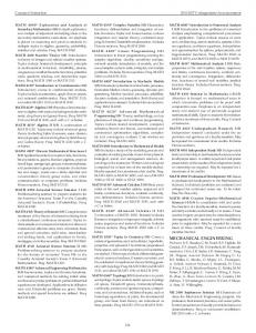
3. Computational conditions In the simulations presented in the next section, stiffness maximization simulations of a cantilever subjected to a concentration force are performed. Figure 1 shows the initial morphology and boundary conditions. The displacements in the x- and y-directions of the nodes along the left end are constrained, and concentrated force P is applied in the ydirection of the node at the center of the right end. The color indicates ; blue represents the material with  = 1, and the hole represents that with  = 0. The computational domain size is 400x × 200x with mesh size x. The initial solid fraction is set to 0.5, and it is maintained during the simulation. A plane stress problem with unit thickness is assumed for the stress field. Time increment t is set to t  x 2 5 2 to stably and explicitly solve Eqs. (21) and (22), and a 10,000-step computation is performed. The boundary conditions for the phase field are set to zero Neumann for all boundaries. The Poisson’s ratio is set to 0.3.





Fig. 1 Initial morphology and boundary conditions for the stiffness maximization simulations of a cantilever where the displacements in the left side are constrained and nodal force P is applied at the center in the right side. The blue region is inside a material with = 1, and the white regions are holes with  = 0.

4. Results and discussion

[DOI: 10.1299/mej.16-00462]


25


4.1 Changes in morphology and stiffness

Figure 2 shows the morphological changes in the simulations for Models A and B under the conditions  = 3x, 1 = 0.25, and 2 = 0.05. Figure 3 shows the variation in the stiffness ratio K/Kini, where stiffness K is defined as K = P/v and Kini is the K for the initial morphology shown in Fig. 1. Here, v is the displacement in the y-direction at the point where P is applied. In Fig. 3, the maximum stiffness during the simulations is shown by the dashed lines. Note that stiffness K is a scalar here. In the computational condition shown in Fig. 1, Eq. (8) can be expressed as F f    ui ti dS  vP   P 2 K . Therefore, minimizing v corresponds to maximizing K. Figure 3 shows some nonS

smooth cusp points. These cusp points are caused by the elimination of members. In the present model, the morphological change simply occurs from a fine to coarse one.

Fig. 2 Morphological changes during the simulations from the initial condition shown in Fig. 1 for Models A and B. (a) 250, (b) 1,000, (c) 2,000, (d) 6,000, and (e) 10,000 steps.

Fig. 3 Variations in stiffness ratio K/Kini during the simulations shown in Fig. 2.

[DOI: 10.1299/mej.16-00462]


26


At the 250th step shown in Fig. 2(a), the topologies in Models A and B are almost the same, although rounded holes are observed in Model A. At the 250th step, the stiffness is almost the same as that shown in Fig. 3. However, at around 400 steps, the differences in the stiffness ratio K/Kini between Models A and B are apparent. Specifically, in Model A, sometimes K/Kini decreases rapidly until 1,000 steps. In Model B, reductions in K/Kini also occur at around 1,000 steps. However, the amount of K/Kini reduction is much smaller in Model B than that in Model A, and the step where the K/Kini reduction starts is delayed for Model B compared with Model A. As a result, the topology of Model A is coarser than that of Model B at the 1,000th step, as shown in Fig. 2(b). From 1,000 to 2,000 steps, the topology of Model B also becomes coarser. Figure 2(c) shows that the topologies of Models A and B become the same at the 2,000th step. On the other hand, Fig. 3 shows the presence of a large difference in K/Kini even for the same topology. In Model A, a small cusp can be seen at around 3,000 steps due to the disappearance of small holes, and temporal large reductions are observed after 6,000 steps due to the disappearance of some holes. Figures 2(c)–(e) show that the morphology of Model A continuously and gradually coarsens. The maximum stiffness of Model A is observed at around 6,000 steps. In Model B, the topologies after 2,000 steps remain the same, as shown in Figs. 2(c)–(e), and the stiffness monotonically increases. From the results shown in Figs. 2 and 3, we conclude that Model B, proposed in this paper, can efficiently increase the stiffness compared with conventional Model A. The differences in the variations in morphology and stiffness between Models A and B are determined by whether the interface migration is driven by the curvature or not. In Model A, the interface migration is driven by the interface curvature, in addition to the strain energy and volume constraint in Model B.

4.2 Effects of 1

Here, we present the investigation of the effects of the amount of 1 on the stiffness change. 1 determines the contribution of strain energy to the value that drives the interface migration. 1 changes from 0.05 to 0.45 with an increment of 0.1 under constant 2 = 0.05. 2 = 0.05 is sufficient to keep the volume within an error of 0.1%. Figure 4 shows the variations in the stiffness ratio K/Kini. Figure 4(a), which shows Model A, illustrates that the maximum stiffness indicated by the filled circles is obtained at different time steps, and the amount of maximum stiffness is different depending on 1. The morphologies of Model A at the maximum stiffness point are shown in the left side of Fig. 5. The figures shown in Fig. 5 are the step numbers that indicate the maximum stiffness. From the figures, we can see that the morphologies that indicate the maximum stiffness are significantly different depending on 1. As for Model B, on the other hand, Fig. 4 shows that the stiffness monotonically increases with time after some perturbations. Therefore, the maximum stiffness for each 1 is obtained at the final 10,000 steps in the present simulations. The maximum stiffness values are the same for large 1, i.e., 1 = 0.25, 0.35, and 0.45. This phenomenon is also observed from the morphologies at 10,000 steps shown in the right side of Fig. 5. According to the final morphologies, the same morphologies are observed at 1 = 0.25, 0.35, and 0.45. In addition, the topology at 1 = 0.15 is the same as those at 1 = 0.25, 0.35, and 0.45. Therefore, if the simulation at 1 = 0.15 is continued much longer, the stiffness and morphology will be the same as those at 1 = 0.25, 0.35, and 0.45. The topology obtained at 1 = 0.05 is coarser than those obtained at other 1 values because the contributions of the strain energy and volume constraint that drive the interface are the same. From the above discussion, we can conclude that stable results that are independent of 1 can be obtained using Model B if we use 1, which is larger than a certain value. From the perspective of computational cost, we can obtain the desired result with a small computational cost by setting 1 larger. In conventional Model A, although we can obtain a high stiffness structure similar to that of Model B when we use larger 1, the results are not stable and largely dependent on the amount of 1.

Fig. 4 Variations in stiffness ratio K/Kini during the simulations for Models A and B when 1 is changed.

[DOI: 10.1299/mej.16-00462]


27


Fig. 5 Morphologies at maximum stiffness ratio K/Kini in Fig. 4 for Models A and B. Here, 1 = (a) 0.05, (b) 0.15, (c)0.25, (d)0.35, and (e)0.45. The figures shown in Model A are the step numbers corresponding to the filled circles in Fig. 4(a).

4.3 Effects of interface thickness  In many AC-type PFTO models, equations similar to Eq. (21) are used. Then, the complexities of a structure are considered to be controlled by the gradient coefficient or  2 . However, changing  2 in Eq. (21) means that both interface thickness and contribution of the curvature in the driving force increase. From the above results, to perform topology optimization using the phase-field method with high accuracy, we can conclude that the phase-field equation should be used, where the curvature contribution is removed from the diffusion term. Here, we show that the structure complexities can be controlled by changing  2 even in Eq. (22). Figure 6 shows the stiffness variations in Model B when the interface thickness is changed, i.e.,  = 2x, 3x, 4x, 5x, and 6x. Here, we use the conditions 1 = 0.45 and 2 = 0.05. In all curves, the stiffness values rapidly increase at the beginning of the simulations and approach an almost constant region with very small but monotonous increase through some preservation because of the topology changes. The final stiffness clearly increases with decreasing interface thickness. Figure 7 shows the morphologies at the final 1.0×104th step shown in Fig. 6. The structures become more complicated as the interface thickness decreases. As shown here, the structure complexities can be controlled by changing the interface thickness in Eq. (22). The morphological change for  = 2x cannot be observed after 900 steps, and the stiffness becomes constant, as shown in Fig. 6. This means that the computation with  = 2x is a little bit unstable. In our experience,  = 3x is the smallest interface thickness to stably compute the PFTO model. Although we can change  2 in Eqs. (21) and (22) to control the complexities of the structure, we believe that changing mesh size x while keeping  = 3x is better for the computational cost and accuracy. If we fix  = 3x, we do not need any other parameter setting except for mesh size x.

[DOI: 10.1299/mej.16-00462]


28


Fig. 6 Variations in stiffness ratio K/Kini during the simulations using Model B with different interface thicknesses  for 1 = 0.45 and 2 = 0.05.

Fig. 7 Morphologies at 1.0×104th step in the simulations shown in Fig. 6:  = (a) 2x, (b)3x, (c) 4x, (d)5x, and (e) 6x.

5. Conclusions In this paper, we have proposed a new phase-field topology optimization (PFTO) model where the curvature effect is removed from the conventional model. By simulating of elastic strain energy minimization under a constant-volume constraint of a cantilever, we have shown that the new model can stably compute the optimum shapes. In other words, the new model can efficiently minimize only the objective function. We can also conclude that by increasing the contribution of the strain energy (or 1 in Eq. (13)), we can reduce the computational cost. In addition, by changing the interface thickness in the new model, we can control the complexities of the final structure. The present method is very simple, but we consider that it is essential and important in the PFTO method. Removing the curvature effects from all previous PFTO models is possible using the method proposed in this study. Therefore, the present method can be considered to be a highly versatile method. If we want to design a rounded-shape structure, we can control the curvature reduction term or Eq. (20) in Eq. (22). In the future, we will use the PFTO model to design the material microstructures in multi-scale and multi-material problems (Kato et al., 2009; Kato et al., 2014) because the phase-field method is excellent at simulating the material microstructures. Therefore, successive simulations of an optimum material microstructure using the PFTO model and phase-field simulations to determine the process to make the optimum material microstructures should be performed. However, in successive simulations of the material microstructures, the conventional PFTO model that includes the curvature effects may be better because curvature effects are naturally included in the material microstructure formations. The PFTO models should be properly used depending on the purposes.

References Allaire, G., Jouve, F. and Toader, A.M., Structural optimization using sensitivity analysis and a level-set method, Journal of Computational Physics, Vol. 194, No. 1 (2004), pp. 363-393.

[DOI: 10.1299/mej.16-00462]


29


Ambati, M., Gerasimov, T. and De Lorenzis, L., A review on phase-field models of brittle fracture and a new fast hybrid formulation, Computational Mechanics, Vol. 55, No. 2 (2015), pp. 383-405. Asta, M., Beckermann, C., Karma, A., Kurz, W., Napolitano, R., Plapp, M., Purdy, G., Rappaz, M. and Trivedi, R., Solidification microstructures and solid-state parallels: Recent developments, future directions, Acta Materialia, Vol. 57, No. 4 (2009), pp. 941-971. Beckermann, C., Diepers, H.J., Steinbach, I., Karma, A. and Tong, X., Modeling Melt Convection in Phase-Field Simulations of Solidification, Journal of Computational Physics, Vol. 154, No. 2 (1999), pp. 468-496. Bendsøe, M.P. and Kikuchi, N., Generating optimal topologies in structural design using a homogenization method, Computer Methods in Applied Mechanics and Engineering, Vol. 71, No. 2 (1988), pp. 197-224. Bourdin, B., Filters in topology optimization, International Journal for Numerical Methods in Engineering, Vol. 50, No. 9 (2001), pp. 2143-2158. Bourdin, B. and Chambolle, A., Design-dependent loads in topology optimization, ESAIM: Control, Optimisation and Calculus of Variations, Vol. 9 (2003), pp. 19-48. Bourdin, B. and Chambolle, A., The Phase-Field Method in Optimal Design, IUTAM Symposium on Topological Design Optimization of Structures, Machines and Materials, Vol. 137 (2006), pp. 207-215. Burger, M. and Stainko, R., Phase-field relaxation of topology optimization with local stress constraints, SIAM Journal on Control and Optimization, Vol. 45, No. 4 (2006), pp. 1447-1466. Chen, L.Q., Phase-field models for microstructure evolution, Annual Review of Materials Science, Vol. 32 (2002), pp. 113-140. Chiu, P.-H. and Lin, Y.-T., A conservative phase field method for solving incompressible two-phase flows, Journal of Computational Physics, Vol. 230, No. 1 (2011), pp. 185-204. Choi, J.S., Yamada, T., Izui, K., Nishiwaki, S. and Yoo, J., Topology optimization using a reaction–diffusion equation, Computer Methods in Applied Mechanics and Engineering, Vol. 200, No. 29–32 (2011), pp. 2407-2420. Dedè, L., Borden, M.J. and Hughes, T.J.R., Isogeometric Analysis for Topology Optimization with a Phase Field Model, Archives of Computational Methods in Engineering, Vol. 19, No. 3 (2012), pp. 427-465. Gain, A.L. and Paulino, G.H., Phase-field based topology optimization with polygonal elements: A finite volume approach for the evolution equation, Structural and Multidisciplinary Optimization, Vol. 46, No. 3 (2012), pp. 327342. Garcke, H. and Hecht, C., Shape and Topology Optimization in Stokes Flow with a Phase Field Approach, Applied Mathematics & Optimization, Vol. 73, No. 1 (2016), pp. 23-70. Karma, A. and Rappel, W.J., Phase-field method for computationally efficient modeling of solidification with arbitrary interface kinetics, Physical Review E - Statistical Physics, Plasmas, Fluids, and Related Interdisciplinary Topics, Vol. 53, No. 4 (1996), pp. R3017-R3020. Kato, J., Lipka, A. and Ramm, E., Multiphase material optimization for fiber reinforced composites with strain softening, Structural and Multidisciplinary Optimization, Vol. 39, No. 1 (2009), pp. 63-81. Kato, J., Yachi, D., Terada, K. and Kyoya, T., Topology optimization of micro-structure for composites applying a decoupling multi-scale analysis, Structural and Multidisciplinary Optimization, Vol. 49, No. 4 (2014), pp. 595-608. Kobayashi, R., Modeling and numerical simulations of dendritic crystal growth, Physica D: Nonlinear Phenomena, Vol. 63, No. 3–4 (1993), pp. 410-423. Kobayashi, R., A Numerical Approach to Three-Dimensional Dendritic Solidification, Experimental Mathematics, Vol. 3, No. 1 (1994), pp. 59-81. Kobayashi, R. and Giga, Y., Equations with singular diffusivity, Journal of Statistical Physics, Vol. 95, No. 5-6 (1999), pp. 1187-1220. Lee, S.S., Tashiro, S., Awazu, A. and Kobayashi, R., A new application of the phase-field method for understanding the mechanisms of nuclear architecture reorganization, Journal of Mathematical Biology, Vol. 74, No. 1 (2017), pp. 333-354. Lim, H., Yoo, J. and Choi, J.S., Topological nano-aperture configuration by structural optimization based on the phase field method, Structural and Multidisciplinary Optimization, Vol. 49, No. 2 (2014), pp. 209-224. Lim, S., Yamada, T., Min, S. and Nishiwaki, S., Topology optimization of a magnetic actuator based on a level set and phase-field approach, IEEE Transactions on Magnetics, Vol. 47, No. 5 (2011), pp. 1318-1321. Miyoshi, E. and Takaki, T., Validation of a novel higher-order multi-phase-field model for grain-growth simulations using

[DOI: 10.1299/mej.16-00462]


10 2


anisotropic grain-boundary properties, Computational Materials Science, Vol. 112 (2016), pp. 44-51. Ohno, M. and Matsuura, K., Quantitative phase-field modeling for dilute alloy solidification involving diffusion in the solid, Physical Review E - Statistical, Nonlinear, and Soft Matter Physics, Vol. 79, No. 3 (2009), pp. 031603. Ohno, M., Tsuchiya, S. and Matsuura, K., Austenite Grain Growth in Peritectic Solidified Carbon Steels Analyzed by Phase-Field Simulation, Metallurgical and Materials Transactions A, Vol. 43, No. 6 (2012), pp. 2031-2042. Osher, S.J. and Santosa, F., Level Set Methods for Optimization Problems Involving Geometry and Constraints I. Frequencies of a Two-Density Inhomogeneous Drum, Journal of Computational Physics, Vol. 171, No. 1 (2001), pp. 272-288. Oshima, K., Takaki, T. and Muramatsu, M., Development of multi-phase-field crack model for crack propagation in polycrystal, International Journal of Computational Materials Science and Engineering, Vol. 03, No. 02 (2014), pp. 1450009. Penzler, P., Rumpf, M. and Wirth, B., A phase-field model for compliance shape optimization in nonlinear elasticity, ESAIM - Control, Optimisation and Calculus of Variations, Vol. 18, No. 1 (2012), pp. 229-258. Rojas, R., Takaki, T. and Ohno, M., A phase-field-lattice Boltzmann method for modeling motion and growth of a dendrite for binary alloy solidification in the presence of melt convection, Journal of Computational Physics, Vol. 298, No. 1 (2015), pp. 29-40. Sakane, S., Takaki, T., Ohno, M., Shimokawabe, T. and Aoki, T., GPU-accelerated 3D phase-field simulations of dendrite competitive growth during directional solidification of binary alloy, IOP Conference Series: Materials Science and Engineering, Vol. 84, No. 1 (2015), pp. 012063. Sethian, J.A. and Wiegmann, A., Structural Boundary Design via Level Set and Immersed Interface Methods, Journal of Computational Physics, Vol. 163, No. 2 (2000), pp. 489-528. Shibuta, Y., Ohno, M. and Takaki, T., Solidification in a Supercomputer: From Crystal Nuclei to Dendrite Assemblages, JOM Journal of the Minerals Metals and Materials Society, Vol. 67, No. 8 (2015), pp. 1793-1804. Steinbach, I., Phase-field models in materials science, Modelling and Simulation in Materials Science and Engineering, Vol. 17, No. 7 (2009), pp. 1-31. Steinbach, I. and Pezzolla, F., A generalized field method for multiphase transformations using interface fields, Physica D: Nonlinear Phenomena, Vol. 134, No. 4 (1999), pp. 385-393. Sun, Y. and Beckermann, C., Sharp interface tracking using the phase-field equation, Journal of Computational Physics, Vol. 220, No. 2 (2007), pp. 626-653. Takada, N., Matsumoto, J. and Matsumoto, S., A Diffuse-interface Tracking Method for the Numerical Simulation of Motions of a Two-phase Fluid on a Solid Surface, The Journal of Computational Multiphase Flows, Vol. 6, No. 3 (2014), pp. 283-298. Takada, N., Misawa, M. and Tomiyama, A., A phase-field method for interface-tracking simulation of two-phase flows, Mathematics and Computers in Simulation, Vol. 72, No. 2–6 (2006), pp. 220-226. Takaki, T., Development of Phase-Field Topology Optimization Model and Its Fundamental Performance Evaluations, Transactions of The Japan Society of Mechanical Engineers Series A, Vol. 77, No. 783 (2011), pp. 1840-1850 (in Japanese). Takaki, T., Phase-field modeling and simulations of dendrite growth, ISIJ International, Vol. 54, No. 2 (2014), pp. 437444. Takaki, T., Hasebe, T. and Tomita, Y., Two-dimensional phase-field simulation of self-assembled quantum dot formation, Journal of Crystal Growth, Vol. 287, No. 2 (2006), pp. 495-499. Takaki, T., Hirouchi, T. and Tomita, Y., Phase-field study of interface energy effect on quantum dot morphology, Journal of Crystal Growth, Vol. 310, No. 7-9 (2008), pp. 2248-2253. Takaki, T., Nakagawa, K., Morita, Y. and Nakamachi, E., Phase-field modeling for axonal extension of nerve cells, Mechanical Engineering Journal, Vol. 2, No. 3 (2015a), pp. 15-00063-00015-00063. Takaki, T., Ohno, M., Shimokawabe, T. and Aoki, T., Two-dimensional phase-field simulations of dendrite competitive growth during the directional solidification of a binary alloy bicrystal, Acta Materialia, Vol. 81 (2014), pp. 272283. Takaki, T., Rojas, R., Ohno, M., Shimokawabe, T. and Aoki, T., GPU phase-field lattice Boltzmann simulations of growth and motion of a binary alloy dendrite, IOP Conference Series: Materials Science and Engineering, Vol. 84, No. 1 (2015b), pp. 012066.

[DOI: 10.1299/mej.16-00462]


11 2


Takaki, T., Shimokawabe, T., Ohno, M., Yamanaka, A. and Aoki, T., Unexpected selection of growing dendrites by verylarge-scale phase-field simulation, Journal of Crystal Growth, Vol. 382 (2013), pp. 21-25. Takezawa, A. and Kitamura, M., Phase field method to optimize dielectric devices for electromagnetic wave propagation, Journal of Computational Physics, Vol. 257 (2014), pp. 216-240. Takezawa, A., Nishiwaki, S. and Kitamura, M., Shape and topology optimization based on the phase field method and sensitivity analysis, Journal of Computational Physics, Vol. 229, No. 7 (2010), pp. 2697-2718. Tavakoli, R., Multimaterial topology optimization by volume constrained Allen–Cahn system and regularized projected steepest descent method, Computer Methods in Applied Mechanics and Engineering, Vol. 276 (2014), pp. 534-565. Tsukada, Y., Koyama, T., Murata, Y., Miura, N. and Kondo, Y., Estimation of /’ diffusion mobility and threedimensional phase-field simulation of rafting in a commercial nickel-based superalloy, Computational Materials Science, Vol. 83 (2014), pp. 371-374. Tsukada, Y., Murata, Y., Koyama, T., Miura, N. and Kondo, Y., Creep deformation and rafting in nickel-based superalloys simulated by the phase-field method using classical flow and creep theories, Acta Materialia, Vol. 59, No. 16 (2011), pp. 6378-6386. Wallin, M. and Ristinmaa, M., Howard's algorithm in a phase-field topology optimization approach, International Journal for Numerical Methods in Engineering, Vol. 94, No. 1 (2013), pp. 43-59. Wallin, M. and Ristinmaa, M., Finite strain topology optimization based on phase-field regularization, Structural and Multidisciplinary Optimization, Vol. 51, No. 2 (2015), pp. 305-317. Wang, M. and Zhou, S., Synthesis of shape and topology of multi-material structures with a phase-field method, Journal of Computer-Aided Materials Design, Vol. 11, No. 2-3 (2004a), pp. 117-138. Wang, M.Y., Wang, X. and Guo, D., A level set method for structural topology optimization, Computer Methods in Applied Mechanics and Engineering, Vol. 192, No. 1–2 (2003), pp. 227-246. Wang, M.Y. and Zhou, S., Phase field: A variational method for structural topology optimization, CMES - Computer Modeling in Engineering and Sciences, Vol. 6, No. 6 (2004b), pp. 547-566. Wang, Y. and Li, J., Phase field modeling of defects and deformation, Acta Materialia, Vol. 58, No. 4 (2010), pp. 12121235. Warren, J.A. and Boettinger, W.J., Prediction of dendritic growth and microsegregation patterns in a binary alloy using the phase-field method, Acta Metallurgica et Materialia, Vol. 43, No. 2 (1995), pp. 689-703. Wheeler, A.A., Boettinger, W.J. and McFadden, G.B., Phase-field model for isothermal phase transitions in binary alloys, Physical Review A, Vol. 45, No. 10 (1992), pp. 7424-7439. Yamada, T., Izui, K., Nishiwaki, S. and Takezawa, A., A topology optimization method based on the level set method incorporating a fictitious interface energy, Computer Methods in Applied Mechanics and Engineering, Vol. 199, No. 45–48 (2010), pp. 2876-2891. Yamanaka, A., Aoki, T., Ogawa, S. and Takaki, T., GPU-accelerated phase-field simulation of dendritic solidification in a binary alloy, Journal of Crystal Growth, Vol. 318, No. 1 (2011), pp. 40-45. Yamanaka, A., Takaki, T. and Tomita, Y., Elastoplastic phase-field simulation of martensitic transformation with plastic deformation in polycrystal, International Journal of Mechanical Sciences, Vol. 52, No. 2 (2010), pp. 245-250. Zhou, S. and Wang, M., Multimaterial structural topology optimization with a generalized Cahn–Hilliard model of multiphase transition, Structural and Multidisciplinary Optimization, Vol. 33, No. 2 (2007), pp. 89-111. Zhou, S. and Wang, M.Y., 3D multi-material structural topology optimization with the generalized Cahn-Hilliard equations, CMES - Computer Modeling in Engineering and Sciences, Vol. 16, No. 2 (2006), pp. 83-101.

[DOI: 10.1299/mej.16-00462]


12 2