J Mol Model (2002) 8:33–43 DOI 10.1007/s00894-001-0068-3
O R I G I N A L PA P E R
Witold Dzwinel · David A.Yuen · Krzysztof Boryczko
Mesoscopic dynamics of colloids simulated with dissipative particle dynamics and fluid particle model
Received: 16 July 2001 / Accepted: 14 November 2001 / Published online: 31 January 2002 © Springer-Verlag 2002
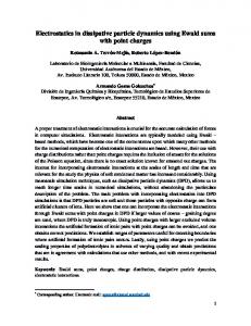
Abstract We report results of numerical simulations of complex fluids, using a combination of discrete-particle methods. Our molecular modeling repertoire comprises three simulation techniques: molecular dynamics (MD), dissipative particle dynamics (DPD), and the fluid particle model (FPM). This type of model can depict multi-resolution molecular structures (see the Figure) found in complex fluids ranging from single micelle, colloidal crystals, large-scale colloidal aggregates up to the mesoscale processes of hydrodynamical instabilities in the bulk of colloidal suspensions. We can simulate different colloidal structures in which the colloidal beds are of comparable size to the solvent particles. This undertaking is accomplished with a two-level discrete particle model consisting of the MD paradigm with a LennardJones (L-J) type potential for defining the colloidal particle system and DPD or FPM for modeling the solvent. We observe the spontaneous emergence of spherical or rod-like micelles and their crystallization in stable hexagonal or worm-like structures, respectively. The ordered arrays obtained by using the particle model are similar to the 2D colloidal crystals observed in laboratory experiments. The micelle shape and its hydrophobic or hydrophilic character depend on the ratio between the scaling factors of the interactions between colloid–colloid to colloid–solvent. Unlike the miscellar arrays, the colloidal aggregates involve the colloid–solvent interactions prescribed by the DPD forces. Different from the assumpElectronic supplementary material to this paper can be obtained by using the Springer LINK server located at http://dx.doi.org/ 10.1007/s00894-001-0068-3 W. Dzwinel (✉) · K. Boryczko AGH University of Mining and Metallurgy, Institute of Computer Science, Kraków, Poland e-mail:
[email protected] Tel.: +48-12-6173520 D. A.Yuen Department of Geology and Geophysics and Minnesota Supercomputing Institute, University of Minnesota, Minneapolis, MN 55415-1227, USA
tion of equilibrium growth, the two-level particle model can display much more realistic molecular physics, which allows for the simulation of aggregation for various types of colloids and solvent liquids over a very broad range of conditions. We discuss the potential prospects of combining MD, DPD, and FPM techniques in a single three-level model. Finally, we present results from large-scale simulation of the Rayleigh–Taylor instability and dispersion of colloidal slab in 2D and 3D. Electronic supplementary material to this paper can be obtained by using the Springer LINK server located at http://dx.doi.org/10.1007/s00894-001-0068-3. Keywords Complex molecular fluids · Fluid particle model · Dissipative particle dynamics · Molecular dynamics simulations · Cross-scale simulations · Phase separation
Introduction The emergence of genuinely new and fascinating phenomena at the nanoscale to mesoscale creates a great need of adequate theory, modeling, and large-scale numerical simulation in order to understand the different regimes of the greatest challenges and opportunities in those transitional regions where nanoscale phenomena are just beginning to emerge from macroscopic and microscale regimes, such as self-assembling amphiphilic mixtures, colloidal suspensions, and porous materials. Today there exist many numerical methods for modeling physical and chemically reacting phenomena in complex molecular fluids. They include molecular dynamics, lattice Boltzmann gas, and cellular automata, [1, 2] diffusion limited aggregation [3, 4] or those employing finite element simulation, e.g., for Cahn–Hillard fluids. [5] Our model falls under the category of the discrete-particle paradigm and comprises three distinct kinds of numerical techniques: molecular dynamics (MD), dissipative particle dynamics (DPD), and fluid particle model (FPM) techniques. The DPD method [6] and its general-
34 Fig. 1 Multiresolution in a complex fluid
ization – the FPM [7] – can provide a bridge between the basic domains of complex fluids, i.e., micelles and colloidal particles, and large-scale structures such as droplets, crystals, colloidal agglomerates, and self-organized patterns from molecular fluid instabilities. The distinct advantage held by DPD over the other methods is the direct possibility for matching the scales of the discrete-particle simulation to the dominant spatiotemporal scales of the entire system. The real cross-scale endeavor, where different kinds of time-steps can be used, reduces then to a proper definition of DPD interactions by using bottom-up [8] or top-down approaches. [9] The fluid particles are represented by the clusters of atoms. As shown in Fig. 1, the relatively narrow gap between the smallest structures and large-scale structures in complex fluids can be connected by using a reasonable number of fluid particles (a hundred thousand in 2D and few millions in 3D) instead of billions of interacting atoms. One disadvantage of DPD is the lack of a drag between the central particle and the second one orbiting in a circumference around the first one. The non-central force, introduced in the FPM, is proportional to the difference between particle velocities and eliminates this defect. However, this makes the model more complex and suggests its use for longer length-scales, where the FPM particle is large enough in that it interacts only with its closest neighbors. The other problem with DPD is that DPD particles
cannot simulate “solid” granular material with attractive forces. The colloidal particles are just such solid grains immersed in a solvent. For simulating suspensions consisting of small number of colloidal beds in which the hydrodynamic interactions between colloidal particles play the dominant role, we can employ the fluid particle dynamics (FPD) approach. [10] In FPD, the colloidal beds are MD particles interacting with Lennard-Jones (L-J) forces. The hydrodynamic interactions are derived from the global velocity field, which is computed directly by integrating the Navier–Stokes fluid dynamical equations. For systems with colloidal beds of a similar size to the complex fluid microstructures (e.g., polymeric clusters, large blood cells) or not much larger, the bed–solvent particle interactions become important. These molecular interactions are responsible for creating colloidal microstructures, such as micelles and colloidal crystals, which cannot be simulated within the framework of FPD. In [11] we attack this problem by employing a twolevel particle model in which the colloidal beds are simulated with MD particles, while the solvent is represented by the DPD model. Because both the colloidal beds and fluid particles are comparable in size, we have employed a uniform time-step in the integration of the Newtonian equation of motion. We will demonstrate the cross-scaling results by simulating complex fluids with a three-level method for
35
which colloidal beds are represented by MD particles but fluid particles – simulated by using DPD and/or FPM interactions – represent a solvent. At first, the three-level method is presented starting from the most general fluid particle model. By introducing two-level model comprising MD and DPD (or FPM) forces, we can simulate miscellar solutions, which undergo crystallization into stable hexagonal or worm-like structures. By merely changing the character of the particle–particle interactions, we can go up the spatio-temporal scale simulating large colloidal aggregates, which involve as many as 20 million particles. On the largest scale, we focus our attention on the Rayleigh–Taylor [12] instability, which induces mixing of the colloidal mixtures and dispersion of the colloidal slab. These simulations are carried out with a three-level method (MD, DPD, and FPM) and with a combined total number of particles in the neighborhood of several million. Finally, we summarize the results and discuss the prospects of the discrete particle method as a computational tool for modeling mesoscopic dynamical phenomena of complex fluid.
Fluid particle model A theoretical framework for the fluid particle model can be found in [7]. The fluid particles, defined by their mass mi, position ri, and velocity vi, interact with each other. The particle can be viewed as a “droplet” consisting of liquid molecules with an internal structure and with some internal degrees of freedom. We use the two-body, short-ranged DPD force F as postulated in [7]. This type of interaction consists of a conservative force FC, two dissipative components FT and FR, and a Brownian force F˜ which are defined by:
tions dependent on the interparticle separation distance r=rij. [7] T – is a dimensionless matrix given by: (6) 1 – is the unit matrix. As proved in [7] the one-component FPM system yields the Gibbs’ distribution as the equilibrium solution to the Fokker–Planck equation under the detailed balance (DB) Ansatz. Consequently it satisfies the fluctuation–dissipation theorem. According to the fluctuation–dissipation theorem the normalized weight functions are chosen such that:
(7) The non-central force in FPM, which is proportional to the difference between particle velocities, introduces an additional drag lacking in the DPD model. The central particle and the second one orbiting around the first one do not produce any force in the DPD algorithm, thus making it inconsistent. The non-central force also results in an additional rotational friction given by Eq. (4). The temporal evolution of the particle ensemble obeys the equations: (8) (9) (10) where the torques in Eq. (10) are given by:
(1) (11) (2) (3) (4)
(5) where: rij – is a distance between particles i and j, rij=ri–rj is a vector pointing from particle i to particle j and eij=rij/rij, D – is spatial dimension, T – is the temperature of particle system, kB – is the Boltzmann constant, dt – is the time-step, γ – is a scaling factor for dissipation forces, ω – is angular velocity, dWS, dWA, tr[dW]1 – are symmetric, antisymmetric, and trace diagonal random matrices of independent Wiener increments defined in [7], A(r), B(r), C(r), , F(r) – are func-
One can verify easily that the total angular momentum is conserved. The main purpose of this model is to generalize both the smoothed particle hydrodynamics method (SPH) [13] – the particle based algorithm used for simulations in macroscale – and dissipative particle dynamics. FPM can predict precisely the transport properties of the fluid, thus allowing one to adjust the model parameters according to the formulas of kinetic theory. Unlike the SPH, the angular momentum is conserved exactly in FPM. The FPM model can thus be interpreted as a Lagrangian prescription of the non-linear fluctuating hydrodynamic equations. [7]
Three-level model The FPM model represents a generalization not only of DPD but also of the MD technique. It can be used as DPD by setting the non-central forces to zero, or as MD
36
by dropping the dissipative and Brownian components. The fluid particle model holds an advantage over DPD but only for larger scales where the particles are adequately large and can interact only with their closest neighbors. In this situation DPD is less efficient because many more particles than for FPM should be involved for creating a drag between circumvented DPD particles. DPD is computationally more efficient than FPM at smaller scales, for which the interaction range (rcut) of the potential must be longer. In the model two types of particles are defined accordingly by: ●
●
Colloidal particles (CP), with an interaction range ≥2.5×λ, where λ is a characteristic length, equal to the average distance between particles. The CP–CP interactions can be simulated by a soft-sphere, energy-conserving potential with an attractive tail. Solvent particles (SP), the “droplets of fluid” located in the closest neighborhood of the colloidal particles and in the bulk solvent. Depending on the interaction range central or non-central forces are included within this framework.
In conventional DLVO theory (Derjaguin, Landau, Verwey, Overbeek) [14] the long-range electrostatic interactions between colloidal spheres can be modeled by a screened-Coulomb repulsion. [15] However, some experimental findings [14, 16] show that like-charged macroions have been attracted to one another by shortranged forces. This phenomenon cannot be explained by conventional theories. The recent simulation results [17] show that the fluctuations of the charge distribution by the small ions result in the attraction between microions. The mean force is a combination of hard-sphere and electrostatic force. As shown in Fig. 2, the L-J force [18] is close to the mean force obtained from large-scale Monte-Carlo calculations performed for a real colloidal mixture. [17] The experimentally measured potential [16] between a pair of 0.65-µm-diameter polystyrene sulfate spheres, which lie very close to an electrically charged glass, is also very similar to the L-J interactions. A better approximation of the colloid–colloid interactions is possible by adding to the L-J force a very steep force with a soft core (see Fig. 2). However, because of simplicity, we will use the shifted and truncated L-J force as a sufficiently accurate approximation for the effective force F(rij) (see Eqs. 16 and 17). We assume that the bulk solvent is simulated by using FPM interactions within an interaction range ≤1.5×λ. Such assumptions allow for the decreasing number of neighbors and shorten the simulation time considerably. A short cut-off radius in DPD simulations generates additional artifacts in the velocity autocorrelation function because hydrodynamic behavior appears only on length scales that involve a relatively large number of particles. [9] For FPM this side effect should be much smaller due to the additional non-central drug force between FPM particles, which is neglected in DPD. The side effects of using a shorter cut-off radius in FPM influences, howev-
Fig. 2 The model of the two-body conservative forces representing the CP–CP interactions
er, the behavior of solvent–colloid mixture. Assuming shorter-ranged FPM interactions between solvent particles in the neighborhood of colloidal particles does not lead to nucleation and formation of micelles. They appear spontaneously, both for DPD and FPM simulations, only within a longer interaction range (≥2.5×λ). For savings in CPU time we also decided to use a simpler DPD force instead of FPM in the neighborhood of colloidal particles. There is no DPD fluid in the system. Interactions between solvent particles are only different in the presence of colloidal particles. Solvent particles interact by using the DPD force (larger cut-off radius) as one of them has at least one colloidal particle in its neighborhood. Otherwise they interact with the FPM force with a shorter cut-off radius. All the interactions are symmetrical and total momentum and kinetic energy are conserved. As shown in [7] DPD and MD are special cases of FPM with some parameters equal to 0. Therefore, the system consisting of solvent and colloidal particles represents the Gibbs equilibrium ensemble provided that FPM multicomponent system does. However, until now there is no formal proof that the multicomponent FPM system is the Gibbs equilibrium ensemble. Such a proof exists only for DPD. [19] We assume here by the analogy that it is also true for FPM. Thus, the three-level system consists of three different procedures, each representing a particular technique of interparticle interactions. Due to the comparable size for the three types of particles, the time-step for integrating the Newtonian equations of motion is uniform. The main assumptions in this model are as follows: 1. We consider here an isothermal system, which consists of M particles. The number of species can easily be generalized for simulating multiphase systems. [19]
37
2. The particle system is simulated inside a rectangular box with periodic or hard wall boundary conditions. Particles of various types can be scattered randomly in the box, i.e., this multi-component system can initially be mixed perfectly, or separated by a sharp interface (stratified, circle, rectangular, random shape). 3. The weight functions in Eqs. (5)–(7) satisfy the conditions imposed. Due to the freedom allowed by the model in selecting the weight functions, we have assumed that: (12) where, rcut – is a cut-off radius, which defines the range of interactions. For r=rij>rcut, Fij=0. The and weight functions from Eq. (5) can be computed from Eqs. (7) and (12). Because of the stochastic nature of the equations of motion for DPD and FPM, finding a suitable numerical scheme is a non-trivial problem. The common integration methods used for DPD simulation (e.g., [20, 21, 22]) are based on a second-order in time-stepping O(dt2) velocity–Verlet scheme. Because the scheme is only an approximation of a stochastic integrator it generates artifacts leading to unphysical correlations and monotonically increasing (or decreasing) temperature drift. In the DPD (and DPD–MD) model we employed a hybrid integrator, which consists of the “leap frog” algorithm in time-stepping for the particles positions and the Adams–Bashforth scheme for the particle velocities. [23] Due to large instabilities observed for angular velocity computations we used the fourth-order equivalent of the hybrid scheme in FPM. [24] As shown in Fig. 3, both the hydrodynamic temperature and hydrodynamic pressures do not exhibit noticeable drift for 1 million time-steps. However, the hydrodynamic temperature is 2% higher than the assumed temperature. This is due to the non-energy conserving scheme applied. As shown in Fig. 3, the detailed balance condition is only slightly violated. For simulations requiring more accurate conservation of thermodynamic quantities, another integrator which uses a thermostat should be considered. The simulation from Fig. 3 was made for the mixture of FPM and L-J particles (with concentration rate 20%) for dimensionless time-step dt=0.05. Moreover, because the conservative interactions dominate over random and dissipative forces in our simulations, the artifacts due to integration schemes are less distinct. The problem of selecting a self-consistent, free of artifacts, and efficient integrator for stochastic and velocity dependent DPD and FPM models remains still open. The values of scaling factors of forces components are approximated by the continuum limit equations. From partial pressure P: (13) [6], we compute the value of Π – the scaling factor for the conservative interactions (Eq. 12). The γ parameter
Fig. 3 Partial pressure Pth and temperature Tth of the 2D FPM particle system with 20% of L-J colloidal particles (the total number of particles M=4.5×10⁴) with time. The initial values for pressure Pth=0.01 (in dimensionless units) and for an assumed temperature T=100 K
of dissipative forces is adjusted according to the formula from kinetic theory: [7] (14) where: νb – is a bulk kinematic viscosity, D – is dimensionality, c2=kBT/m, and (15)
Colloidal arrays With the two-level model (DPD and MD) we can study the molecular dynamics of binary fluids. This system consists of colloidal particles (CPs) immersed in a solvent represented by an ensemble of solvent particles (SPs). The colloidal particles are scattered randomly in the box, i.e., this binary system is initially well mixed. The collision operator for the whole particle system consists of DPD and L-J components, and is given by the formula: (16)
(17) Thus, the CP particles interact with the L-J force with both CPs and SPs particles. Because the forces are short ranged, we use a modified L-J force given by Eqs. (16)
38
Fig. 4 a Worm-like structures in colloidal suspension. b The zoom-in of the coexistence region of the lamellar and of the “hydrophobic” phases. The lamellar microstructures are built of rod-like micelles. The “hydrophobic” phase represents hexagonally arranged spherical micelles with solvent particle in the center (gray) surrounded by colloidal particles (white). The ratio εCP–CP/εCP–SP=5, the number of particles is M=2×10⁴, the number of time-steps is N=106. See the supplementary material for movie (Fig. 4S)
Table 1 Principal parameters of the particle system Entire particle system
DPD fluid CP–CP interactions CP–SP interactions
and (17) vanishing for rij≥rcut, where rcut is a cut-off radius. The dual character of SP particle interactions – dissipative particle dynamics with other SP beads and molecular dynamics with L-J interaction and CP particles – can be explained by assuming that the SP ensemble can simulate a complex fluid. For example, the SP particles can represent parts of polymeric chains whose mutual interactions are modeled by using DPD forces, while the conservative and repulsive–attractive forces are responsible for gluing the chains to the hard-core nano-particles. The fundamental parameters of the particle system are presented in Table 1 in dimensionless units. The size of the system is scaled up to the cut-off radius. The time-step and the mass of colloidal particles are set to 1. The energy unit (εUnit) is set arbitrarily as a reference point for scaling both the L-J CP–CP and CP–SP interactions. It corresponds to the ε parameter of the L-J force. In [11] we show that, depending on the εCP–CP/εCP–SP aspect ratio, different colloidal structures (2D colloidal arrays) can be simulated. Simultaneously we have repeated the calculations by using FPM with rcut=2.5×λ instead of DPD (for FPM with rcut=1.5×λ we do not observe the creation of micelles). The simulations were carried out at different concentrations of CP particles, ranging from 10% to 30%. The results shown below are produced by assuming a concentration of CP particles of 20%. For a low aspectratio configuration we find that the “hydrophilic” circular micelles can self-organize and be formed spontaneously. The micelle is represented by a colloidal particle located in the center and surrounded by solvent particles. The 2D hexagonal colloidal arrays are produced as a consequence. These structures are very common [25] and are observed in laboratory experiments, e.g., see http://www-unix.oit.umass.edu/~dinsmore. By increasing the ratio, the hexagonal phase undergoes a self-organized transition to a lamellar metastable phase (see Fig. 4a and movie). [25, 26] The rod-like micelles from Fig. 4b consisting of linearly arranged colloid particles separated by solvent particles form worm-like arrays (Fig. 4a), as shown on the URL http://chemeng.stan-
Parameter
Value (in dimensionless units)
rc – unit of length ∆t – unit of time M=MCP=MSP – unit of mass n – particle density λ – avg. distance between particles System size in rc units εUnit – unit of energy T0 – temperature of the system Ω – dissipative factor Π – scaling factor for conservative forces εCP–CP – L-J well depth σCP–CP – L-J parameter εCP–SP – L-J well depth σCP–SP – L-J parameter
1 1 1 6.37 0.4 42 4.75×10⁻⁵ 0.1×εUnit 10,100 3.8×10⁻³ 0.2–1.6×εUnit 0.4 0.1–1.6×εUnit 0.4
39
Fig. 5 Colloidal structures of circular “hydrophobic” micelles simulated with two-level model. Only colloidal particles are visible. When we zoom in we can observe the hexagonal order of the micelles (εCP–CP/εCP–SP=16, M=2×10⁴, number of time-steps N=106). See the supplementary material for zoom-in (Fig. 5S)
Fig. 6 Colloidal aggregates simulated with two-level model (M=1.2×10⁶, number of time-steps N=105, 33% colloidal particles 67% fluid). See the supplementary material for zoom-in (Fig. 6S)
ford.edu/~gastgrp/images/dendritic-Xsmall.jpg. The lamellar metastable phase evolves into “hydrophobic” hexagonal arrays, as shown in Fig. 5, which then produce larger aggregates. The clustering of micelles and small nano-particles forming colloidal aggregates plays a very prominent role in the development of new materials with a scale size ranging from nano- to mesoscale. Fractal aggregates represent very fragile mechanical structures, which can be easily torn apart as a result of adequately strong external forces. Therefore, aggregating additives are used for controlling the rheology of paints and other coating systems. At low shear rates these shear-thinning non-Newtonian fluids have a high viscosity and a low viscosity at high shear rates. There are many numerical techniques devised for simulating the colloidal aggregates. Most of these methods employ the Smoluchowski principle of coagulation according to a given reaction scheme. [4, 27] These methods are still far from achieving reality. They are adequate for investigating static fractal structures of large agglomerate by assuming a low initial concentration of colloidal particles. For denser systems, the rheological properties of solvent and the mechanisms of aggregation vary tremendously with the particle concentration, which cannot be predicted with simple composite theories. [16] As shown in Fig. 5, the two-level method fits in very well in fine-grained structures during the initial aggregation. However, the method is too computationally demanding for investigating large structures. More reliable statistics are required for monitoring the global properties of the growth process. We propose an alternative approach for simulating large aggregates, which will entail modifying the collision operator given in Eq. (17).
Going up to a larger spatio-temporal scale, we can assume CP particles can be represented not by hard-core beads but by the micelles. The SP particles are the DPD “droplets” of a complex liquid solvent of the size of CPs. At this time the CP particle interactions assume a dual character. In order to avoid fluidization of the colloidal particle system and allow them to aggregate, we have insisted that the colloid–colloid interactions should possess a hard-sphere core with a very short-ranged adhesive part. [28] The soluble additives are excluded from a region, which is comparable to their own size near the particle surface. Consequently a depletion force is produced, [29] which is of entropic origin. For the sake of simplicity, we have assumed here that CP–CP interactions can be modeled by an L-J force, as it was in the colloidal crystals case. In order to tune the system better, we can employ more realistic depletion potentials [15] or tabularized experimentally measured potentials. [16] Unlike the case of miscellar arrays, the CP–SP interactions are simulated by employing DPD forces. This can be justified on the grounds that now the SP beads represent “droplets” of complex fluid, but not the fragments of polymeric chain. Because the CP “droplet” contains a hard core, we have modified the repulsive portion of the conservative FC CP–SP forces. This makes the potential to be steeper than that for the SP–SP interactions. In Fig. 6 we present a snapshot from MD–DPD simulation of a developed colloidal aggregate. By zooming into a particular region of this frame, we can see clearly the hexagonal structure of the aggregated body. Employing the two-level model, [30] we have studied the scaling properties of mean cluster size S(t), expressed in number of particles versus time, by assuming a high concentration of colloidal particles in the system. For the
40
Due to rotational diffusion in FPM, application of the MD–FPM two-level model for a high concentration of the CP particles should accelerate the initial agglomeration process. However, the time required for formation of the seeds is very short (about 1000 time-steps, comparing to a total simulation time about 105 time-steps). It is much shorter than the time needed for producing the miscellar phase. Therefore, we may expect that for the same resolution the MD–FPM model would be not as efficient as the combined MD–DPD scheme.
Multiresolution structures developed in mixing induced by the Rayleigh–Taylor instability
Fig. 7 a The mean cluster size S(t) and b the largest cluster size Smax in time for different CP concentrations. The M=1.2×10⁶ particles were simulated. Linear fits with κ≈0.5, κ≈1 are depicted in a
cases of non-cohesive systems, with a low concentration of colloidal beads, the asymptotic growth for t→∞ of the mean cluster size S(t) is given by: (18) where κ is the scaling-law index. We show that in a dissipative solvent of high concentration of colloidal particles, the growth of mean cluster size can be described by the power law S(t)∝tκ (see Fig. 7a). We have found the intermediate DLA regime, for which κ=1/2. It spans for a relatively long time. The intermediate regime depends on physical properties of the solvent such as the viscosity, temperature, and partial pressure. The character of cluster growth varies with time and the exponent κ shifts at longer time scales from 1/2 to ≈1. This result agrees with the theoretical predictions for diffusion-limited cluster–cluster aggregation, which state that for t→∞ the value of κ=1 for a low colloidal particle concentration. Instead, we show in Fig. 7b that this process cannot be asymptotic with time for larger CP concentrations.
The great advantages of the three-level model become obvious in the simulation of multiscale phenomena associated with the mixing induced by the Rayleigh–Taylor instability. This process involves the CP particles in the solvent. Let us assume that the upper part of the computational box is filled up with heavy (H) CP particles and the lower part with lighter (L) SP solvent particles. The heavy layer is ten times thinner than the lighter one. The collision operator is given by Eqs. (16) and (17). By using MD–DPD model for a medium sized particle system comprising M=106 particles of both types, we need one IBM-SP processor running 1 week for integrating 105 time-steps. However, by using MD–DPD model (with rcut=2.5×λ) more than 90% DPD particles simulating the solvent will not contribute to the small-scale phenomena occurring on the CP–SP interface. Therefore, it is reasonable to employ FPM with a shorter cut-off radius (rcut=1.5×λ) in order to reduce greatly the computational time spent for calculating SP–SP interactions. We assume that SP particles will interact as DPD (with rcut=2.5×λ) being only in the closest neighborhood of CP particles. The parameters of DPD and FPM interactions were matched by using the kinetic theory equations [7] for the same transport coefficients. The same solvent particle can assume dual roles (DPD or FPM), depending on whether CP particle lies within the interaction range. In Fig. 8a and its zoomed-out portion we show both the large-scale Rayleigh–Taylor patterns and the smallscale nucleation of crystallites in the front of CP spikes. As displayed in Fig. 8b, in the beginning the number of micelles increases slowly on the CP–SP interface due to diffusion. The nucleation process is accelerated in the non-linear regime of the Rayleigh–Taylor instability. The length of the interface separating two immiscible DPD fluids during the mixing induced by the Rayleigh–Taylor instability increases as t2. [31] The nucleation process becomes faster. The number of micelles increases with time as tk with k approximately equal to 5/2. The particular value of k does not depend on the temperature of the system. Since the CP–SP interactions do not have any singularities and can be described by FPM-like forces, we can investigate the dispersion of colloidal agglomerate in fluid over the mesoscale. Unlike in the liquid–liquid case in
41
which the mixing starts spontaneously by the thermal fluctuations, the solid–liquid system does not mix so well. This is due to the energy dissipated in colloidal systems and the resistance offered to the mixing by the attractive molecular forces. The fragmentation occurs provided that the colloidal system is permeable and undergoes excessive wetting. Three types of fragmentation structures are found: rupture, erosion, and shatter. [32] The microstructures produced during mixing are completely different from the bubbles and spikes detected in classical Rayleigh–Taylor instability. [12] Instead, one can observe multi-scale structures consisting of large fishbone clusters made of a long threads or more oblate agglomerates. The snapshots from simulations involving more than 1 million particles are displayed in Fig. 9a,b,c. One can discern the places where more vigorous flow occurs, producing slender thread-like structures. The fishbone fragmentation of large clusters, as shown in Fig. 9a,b, is caused by the flow dynamics. We depict in Fig. 10a how the threads go along with the flow streamlines, while the oblate aggregates are found in stagnant regions. After a period of vigorous fragmentation, the energy of flow damps out and the threads shrink and then agglomerate. The aggregation of colloidal beds occurs due to collisions between the aggregates, which are perturbed by the flow, or due to cohesion forces. The fishbone structures in this mixing process come from a quasi-equilibrium situation due to the dynamical encounter between the colloidal particles and the overall flow induced by the global fluid dynamics. The shatter mechanism of slab fragmentation is depicted in Fig. 10b. Due to high Fig. 8 a The formation of hexagonal structures of circular micelles – created by one solvent particle in the center (gray) surrounded by colloidal particles (black) – is observed in front of the spikes. See the supplementary material to observe the difference in scales. b The plot shows the number of micelles in time for twoparticle systems at different temperatures
Fig. 9 a A snapshot from simulation of an accelerated colloidal cluster falling in a long box in 2D (about 1 million particles are simulated). b The zoom-in of a part of Fig. 9a. c The snapshot from respective simulation in 3D (two million particles are simulated). The MD–FPM models were employed
42
pic methods used for complex fluid simulation. These advantages are: 1. The three-level model is a homogeneous, particlebased model, which can operate over diverse spatiotemporal scales, which extend from a micelle, colloidal crystals, droplets, to large-scale features. 2. This model is consistent with the nonlinear fluctuating hydrodynamic equations. [7, 33, 34] Since thermal noise is introduced consistently, it can be used for studying non-equilibrium thermal fluctuations in hydrodynamic systems. 3. The particles evolve in a gridless fashion in real-time, thus allowing for a real-time, realistic visualization. The principal results obtained in the modeling of complex fluids with discrete particles can be summarized as follows :
Fig. 10 a A snapshot from simulation of the mixing induced by the Rayleigh–Taylor instability in 2D. Fragmentation and agglomeration patterns can be easily observed. For the 2D picture the Huygens System 2.2.1 [http://www.svi.nl/] was implemented for data extraction. The densest regions are in dark blue and green, and the regions of the lowest density in dark red. b Fragmentation of a colloidal slab for MD–DPD two-level model in 3D. The colloidal slab accelerated in 3D cubic box is fragmented due to the shatter mechanism. See the supplementary material for movie (Fig. 10S)
energy load caused by compression and decompression the colloidal slab is fragmented instantly into many small pieces, which after some time slowly agglomerate in larger clusters.
Concluding points Our discrete-particle simulations have clearly revealed the prospects of the three-level model comprising MD, DPD, and FPM. We have delineated the many significant advantages of the three-level model over other mesosco-
1. Using a two-level model consisting of DPD and MD, we have observed the creation of colloidal crystals with different phases: “hydrophilic”, lamellar and “hydrophobic”. By changing the balance of the scaling factors in the CP–SP and CP–CP interactions, we can discern clearly the transition of one phase to the other. Metastable regimes with two phases in coexistence are detectable. 2. By changing the character of the CP–SP interactions from conservative to dissipative, we can investigate the dynamics of colloidal aggregates. We show that in the dissipative solvent with high concentration of colloidal particles, the growth of mean cluster size can be described by the power law S(t)∝tκ. In the intermediate DLA regime, for which κ=1/2, this lasts for a long time. The character of cluster growth varies with time and the exponent κ shifts at longer times from 1/2 to ≈1. We show that this process cannot approach an asymptotic limit in time for larger CP concentrations. 3. The three-level (MD–DPD–FPM) simulation of mixing associated with the Rayleigh–Taylor instability of colloidal particles in a solvent shows that the colloidal arrays may appear not only in the well mixed colloidal suspension but also on the mixing front. An increase in the number of micelles in time during mixing occurs faster than the increase in the length of the CP–SP interface. 4. In simulating the dispersion of a colloidal slab, three types of fragmentation structures can be developed: rupture, erosion, and shatter. In [35] the conception of the “higher level” generic DPD paradigm was presented. This model is more general and thermodynamically consistent than FPM – the volume of particle, internal energy, and entropy of the particle system are variable. Our criticism of this model bases mainly on its computational complexity. The “generic” DPD has a greater number of implicit variables than for FPM. The selection of a numerical integrator for the resulting stochastic differential equations to be sufficiently reliable, fast, and convergent for a large number of time-
43
steps is not a trivial problem. Due to additional computational load generated by more sophisticated numerical schemes the “generic” DPD model is still too slow to be competitive with FPM code. The “generic” (multiscale) DPD model was accomplished for a one-component fluid. Its extension to a multi-component fluid is not as straightforward as for the “classical” DPD [19] and as intuitive as for FPM. As we have shown in [24] the standard procedures of parallelization of MD codes applied for FPM model yields surprisingly low speedups, probably because of cache problems. The “generic” DPD model is much more sophisticated than FPM. Before implementing of the new “generic” DPD, the problems with efficient parallelization of FPM should be solved. All of these factors lead to the degradation of computational performance for the “generic” DPD. The model, though very promising for future multiscale simulations of real fluids, is still too complex for standard simulations involving more than 1 million particles in 3D. In our opinion FPM (combined with DPD and MD) meets current computational possibilities better as it is competitive with other mesoscopisc techniques such as lattice Boltzman gas and direct simulation Monte-Carlo. Summarizing, simulation techniques such as DPD and FPM can be employed to study the thermal transport rates in fluids by the suspension of nanoparticles in them, because there is at present no real understanding of the mechanisms by which nanoparticles alter thermal transport in fluids. Today we have an urgent need to understand physical and chemical processes involving nanoscale structures, since society is faced with deadly phenomena involving the trapping and release of contaminants and pathogens. Many of these are in the form of aerosol and colloidal structures, which provide sites for complicated interactions with microbes that control or mediate the bioavailability of a wide variety of organic and inorganic materials in the mesoscale. All of these phenomena can be attacked by using the mesoscopic techniques based on interacting particles. Supplementary material In the supplementary material it is possible to zoom in on several figures, and for other ones movies are available. Acknowledgements We thank Dr Dan Kroll from Minnesota Supercomputing Institute for his contribution to this work. Support for this work has been provided by the Energy Research Laboratory Technology Research Program of the Office of Energy Research of the U.S. Department of Energy under subcontract from the Pacific Northwest National Laboratory and Polish Committee of Scientific Research (KBN) T11 project.
References 1. Rothman DH, Zaleski S (1997) Lattice-gas cellular automata: simple models of complex hydrodynamics. Cambridge University Press, London 2. Chopard B, Droz M (1998) Cellular automata modeling of physical systems. Cambridge University Press, London 3. Kremer K (2000) In: Cates ME, Evans MR (eds) Soft and fragile matter. Proceedings of the Fifty Third Scottish Universities Summer School in Physics. A NATO Advanced Study Institute 4. Meakin P (1998) Fractals, scaling and growth far from equilibrium. Cambridge University Press 5. Cahn JW, Hillard JE (1958) J Chem Phys 28:258–267 6. Hoogerbrugge PJ, Koelman JMVA (1992) Europhys Lett 19:155–160 7. Español P (1998) Phys Rev E 57:2930–2948 8. Flekkøy EG, Coveney PV (1999) Phys Rev Lett 83:1775– 1778 9. Español, P, Serrano M (1999) Phys Rev E 59:6340–7 10. Tanaka H, Araki T (2000) Phys Rev Lett 85:1338–1341 11. Dzwinel W, Yuen DA (2000) J Colloid Interface Sci, 225: 179–190 12. Taylor GI (1950) Proc R Soc London, Ser A 201:192–201 13. Libersky LD, Petschek AG, Carney TC, Hipp JR, Allahdadi FA (1993) J Comput Phys 109:67–73 14. Grier DG, Behrens SH (2001) In: Holm C Keikchoff P, Podgornik R (eds) Electrostatic effects in soft matter and biophysics. Kluwer, Dordrecht 15. Daniel JC, Audebert R (1999) In: Daoud M, Williams CE (eds) Soft matter physics. Springer, Berlin Heidelberg New York 16. Larson RG (1999) The structure and rheology of complex fluids. Oxford University Press, New York 17. Prausnitz J, Wu J (2000) En Vision 16:18–19 18. Haile PM (1992) Molecular dynamics simulation. Wiley, New York 19. Coveney PV, Español P (1997) J Phys A: Math Gen 30: 779–784 20. Coveney PV, Novik KE (1996) Phys Rev E 54:5134–5141 21. Novik KE, Coveney PV (1997) Int J Mod Phys C 8:909–915 22. Groot RD, Warren PB (1997) J Chem Phys 107:4423 23. Dzwinel W, Yuen DA (2000) Int J Mod Phys C 11:1–25 24. Boryczko K, Dzwinel W, Yuen DA (2002) Concurrency and Computation: Practice and Experience 14:1–25 25. Taupin C (1999) In: Daoud M, Williams CE (eds) Soft matter physics. Springer, Berlin Heidelberg New York 26. Poon W (2000) In: Cates ME, Evans MR (eds) Soft and fragile matter. Proceedings of the Fifty Third Scottish Universities Summer School in Physics, A NATO Advanced Study Institute 27. Meakin P (1988) Adv Colloid Interface Sci 28:249–331 28. Gast AP, Russel WB (1998) Phys Today 12:24–30 29. Yaman K, Jeppesen C, Marques CM (1998) Europhys Lett 42:221–226 30. Dzwinel W, Yuen DA (2000) Int J Mod Phys C 11:1037–1061 31. Dzwinel W Yuen DA (2001) Int J Mod Phys C 12:91–118 32. Ottino JM, De Roussel P, Hansen S, Khakhar DV (2000) Adv Chem Eng 25:105–204 33. Breuer HP, Petruccione FA (1993) Physica A 192:569–588 34. Marsh C, Backx G, Ernst MH (1997) Phys Rev E 56:1976 35. Español P, Serrano M, Ottinger HCh (1999) Phys Rev Lett 83:4542–4545