MLP and Elman Recurrent Neural Network Modelling for the TRMS S. F. Toha1 and M. O. Tokhi Department of Automatic Control and Systems Engineering, The University of Sheffield, UK
[email protected] Abstract—This paper presents a scrutinized investigation on system identification using artificial neural network (ANNs). The main goal for this work is to emphasis the potential benefits of this architecture for real system identification. Among the most prevalent networks are multi-layered perceptron NNs using Levenberg-Marquardt (LM) training algorithm and Elman recurrent NNs. These methods are used for the identification of a twin rotor multi-input multi-output system (TRMS). The TRMS can be perceived as a static test rig for an air vehicle with formidable control challenges. Therefore, an analysis in modeling of nonlinear aerodynamic function is needed and carried out in both time and frequency domains based on observed input and output data. Experimental results are obtained using a laboratory set-up system, confirming the viability and effectiveness of the proposed methodology. Keywords—Multi layer perceptron neural network (MLP-NN), Levenberg-Marquardt, twin rotor MIMO system (TRMS), Elman neural network.
I.
INTRODUCTION
Soft computing refers to a consortium of computational methodologies. Some of its principal components include Fuzzy logic (FL), Neural networks (NNs) and genetic algorithms (GAs), all having their roots in artificial intelligence (AI). In today’s highly integrated world, when solutions to problems are cross-disciplinary in nature, soft computing promises to become a powerful means for obtaining solutions to problems quickly, yet accurately and acceptably. In the triumvirate of soft computing, NNs are concerned with adaptive learning, non-linear function approximation, and universal generalization. Neural networks are simplified models of the biological nervous system and therefore have drawn their motivation from the kind of computing performed by a human brain. An NN in general is a highly interconnected network of a large number of processing elements called neurons in an architecture inspired by the brain. An NN can be massively parallel and therefore is said to exhibit parallel distributing processing. There has been an explosion in the literature on NNs in the last decades or so, whose beginning was perhaps marked by the first IEEE International Conference on Neural Networks in 1987. It has been recognised that NNs offer a number of potential benefits for applications in the field of control
engineering, particularly for modelling non-linear systems. Some appealing features of NN are its ability for learning through examples, they do not require any a priori knowledge and can approximate arbitrary well any non-linear continuous function [1]. A number of techniques and interesting discussions of NNs from a system identification viewpoint have been provided in the literature, [2]-[5]. This research will present a method of system modelling using non-parametric identification techniques where NN is utilized. The first part of the paper will explain the NN architecture based on multi-layer perceptron (MLP). Levenberg-Marquardt learning algorithms are used to train the empirical model. The second part will describe Elman recurrent NN. The responses of all the experimental based models are compared with those of the real TRMS to validate the accuracy of the model. Hence, the performances of the models are also compared with respect to each other. The models obtained for the TRMS will be used in subsequent investigations for the development of dynamic simulation, vibration suppression and control of the twin rotor system. II.
TWIN ROTOR MIMO SYSTEM
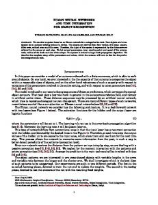
The TRMS used in this work is shown in Fig. 1. It is driven by two DC motors. Its two propellers are perpendicular to each other and joined by a beam pivoted on its base that can rotate freely in the horizontal and vertical planes. The beam can thus be moved by changing the input voltage in order to control the rotational speed of the propellers. The system is equipped with a pendulum counterweight hanging from the beam, which is used for balancing the angular momentum in steady-state or with load. The system is balanced in such a way that when the motors are switched off, the main rotor end of the beam is lowered. The controls of the system are the supply voltages of the motors. It is important to note that the geometrical shapes of the propellers are not symmetric. Accordingly, the system behaviour in one direction is different from that in the other direction. Rotation of a propeller produces an angular momentum which, according to the law of conservation of angular momentum, is compensated by the remaining body of the TRMS beam. This results in interaction between the moment of inertia of the motors with propellers. This interaction directly influences the velocities of the beam in
Authorized licensed use limited to: Sheffield University. Downloaded on July 15, 2009 at 09:44 from IEEE Xplore. Restrictions apply.
both planes. The measured signals are: position of the beam, which constitute two position angles, and the angular velocities of the rotors. Angular velocities of the beam are software reconstructed by differentiating and filtering the measured position angles of the beam. Yaw Axis
ϕ Rotational Angle Main Rotor Tail Rotor
of activation functions such as threshold, piecewise linear, sigmoid, tansigmoid and Gaussian are used for activation. An MLP is an adaptive network whose nodes or neurons perform the same function on incoming signals; this node function is usually the composite of the weighted sum and a differentiable non-linear activation function, also known as transfer function [7]. Fig. 3 shows a structure of a neuron in an MLP network. All neurons, except those in the input layer, perform two functions. They act as a summing point for the input signals as well as propagating the input through a non-linear processing function.
Pitch Axis
θ Elevation Angle Counterbalance
p(1)
Σ
p(2)
1
Σ
F2
1
Σ
F3
1
Σ
F1
Σ
F2
Σ
F3
#
1
#
1
#
1
#
p(4)
Σ
F1
Σ
F2
Σ
F3
p(3) TRMS 33-220
F1
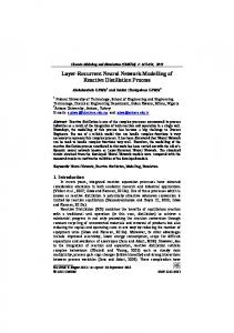
Figure 1. Twin rotor MIMO system Figure 2. Architectural graph of MLP with three hidden layers
III.
X1
MODELLNG WITH NEURAL NETWORK
Neural network is commonly employed for nonlinear modeling of a system. Neural networks possess various attractive features such as massive parallelism, distributed representation and computation, generalization ability, adaptability and inherent contextual information processing [6]. Due to the efficient nature of its working principles and other attractive characteristics, this work is focusing on the use of NNs for the purpose of system identification. Among the various types of artificial NNs (ANNs), the MLP and recurrent NNs are commonly utilized in identification and control of dynamic systems. A. Multi-layer Perceoptron Neural Network Multi layer perceptron neural network consists of a set of sensory units that constitute the input layer, one or more hidden layers of computation nodes and an output layer of computation nodes. The input signal propagates through the network in a forward direction, on a layer-by-layer basis. Fig. 2 shows the architectural graph of an MLP NN with two hidden layers. The model of each neuron in the MLP network includes nonlinearity at the output end. MLP network architecture form a wide set of feed-forward neural networks. Adaptability of the neural models for any application provides by training procedures. The layer, to which the input data is supplied, is called the input layer and the layer from which the output is taken is known as the output layer. All other intermediate layers are called hidden layers. The layers are fully interconnected which means that each processing unit is connected to every unit in the previous and succeeding layers. However, the units in the same layer are not connected to each other. A neuron, as a basic unit of the network, performs two functions: the combining function and the activation function. Different types
w1 j
X2
X3
w2 j
Σ
w3 j
f (.)
Yi
Node j
Xn
wnj
Figure 3. Node j of an MLPNN
The most commonly training methods in MLP is error backpropagation (BP) algorithm [8,9]. In spite of the fact that BP is successfully used for various kinds of tasks, it have lacks such as slow convergence, non-stability of convergence and local minimum problem [10]. The NN with standard backpropagation learning method may get stuck in a shallow local minimum as the algorithm is based on the steepest descent (gradient) algorithm. Since the local minimum is surrounded by a higher ground, and once entered, the network usually does not leave a local minimum with a standard backpropagation algorithm. Therefore, a highly popular algorithm known as the Levenberg-Marquardt algorithm is employed to enable the MLP-NN to slide through local minima and converge faster. A full description of Levenberg-Marquardt algorithm can be found in [11]. The algorithm can be considered as a modified version of Gauss-Newton approach. Like all other training algorithms the first step is initialization. The Jacobian matrix is calculated using the derivative of each error ei with respect to each weight w or bias and consequently the result will be an N × n matrix;
Authorized licensed use limited to: Sheffield University. Downloaded on July 15, 2009 at 09:44 from IEEE Xplore. Restrictions apply.
⎡ ∂e1 ( w) ⎢ ∂w 1 ⎢ ∂ e ( ⎢ 2 w) J ( w(t )) = ⎢ ∂w1 ⎢ # ⎢ ∂e ( w) ⎢ n ⎢⎣ ∂w1
∂e1 ( w) ∂w2 ∂e2 ( w) ∂w2 # ∂en ( w) ∂w2
∂e1 ( w) ⎤ ∂wn ⎥ ⎥ ∂e2 ( w) ⎥ " ∂wn ⎥ % # ⎥ ∂en ( w) ⎥ " ⎥ ∂wn ⎥⎦ "
(1)
Thus, a set of equations is defined in order to find Δw(t ) .
[
Δw(t ) = J T ( w) J ( w) + μI
]
−1
J T ( w)e( w)
(2)
The new sum square error is then computed and compared to the previous one. If the performance becomes better, where the new error is less than the previous one, then the new parameters are defined as:
w(t + 1) = w(t ) + Δw(t ) and the parameter
μ is decreased using μ =
(3)
μ β
. The new
iteration is started if the stop criteria are not satisfied, otherwise μ is increased using μ = μβ and Δw(t ) is recalculated. B. Elman Recurrent Neural Network Recently, substantial research efforts were devoted showing that recurrent neural networks are effective in modelling nonlinear dynamical systems [12-18]. The use of recurrent neural networks (RNN) as system identification networks and feedback controllers offers a number of potential advantages over the static layered networks. RNN provide a means for encoding and representing internal or hidden state, albeit in a potentially distributed fashion which leads to capabilities that are similar to those of an observer in modern control theory. Moreover, RNN is capable of providing long range predictions even in the presence of measurements noise and provide increasing flexibility for filtering noisy inputs [19]. RNN with internal dynamics are adopted in several recent works. Models with such network are shown [20-22], to have the capability of capturing various plant nonlinearities. They have been shown more efficient than feedforward NN in terms of the number of neurons required to model a dynamic system [23, 24]. Recurrent neural networks are different from feedforward network architecture in the sense that there is at least one feedback loop. Thus in this networks, there could exist one layer with feedback connections as well as there could also be neurons with self feedback link where the output of a neuron is fed back into itself as the input. The presence of feedback loop has a profound impact on the learning capability of the network. Furthermore, these feedback loops involve the use of
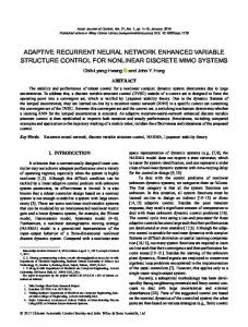
particular branches composed of unit delay elements that result in nonlinear dynamical behaviour by virtue of the nonlinear nature of neurons. Nonlinear dynamics has a key role in the storage function of a recurrent network [25]. Contrary to feedforward networks, recurrent networks can be sensitive, and be adapted to past inputs. Among the several NN architectures found in the literature, recurrent NNs (RNNs) involving dynamic elements and internal feedback connections have been considered as more suitable for modelling and control of non-linear systems than feedforward networks [26]. Elman [27] has proposed a partially RNN, where the feedforward connections are modifiable and the recurrent connections are fixed. It occupies a set of context nodes to store the internal states. Thus, it has certain unique dynamic characteristics over static NNs, such as the MLP-NN and radial basis function (RBF) networks [28]. The connections are mainly feedforward but also include a set of carefully chosen feedback connections that allow the network to remember cues from the recent past. The input layer is divided into two parts that are the true input units and the context units that hold a copy of the activations of the hidden units from the previous time step. As the feedback connections are fixed, backpropagation can be used for training of the feedforward connections. The network is able to recognize sequences and also to produce short continuations of known sequences [27]. The structure of the Elman NN (ENN) is illustrated in Fig. 5 −1
where z is a unit delay. The Elman network has tansig neurons in its hidden (recurrent) layer, and purelin neurons in its output layer. This combination is special in that two-layer networks with these transfer functions can approximate any function (with a finite number of discontinuities) with arbitrary accuracy. The only requirement is that the hidden layer must have enough neurons. More hidden neurons are needed as the function being fitted increases in complexity [29]. It is easy to observe that the Elman network consists of four layers: input layer, hidden layer, context layer, and output layer. There are adjustable weights connecting each two adjacent layers. Generally, it can be considered as a special type of feedforward NN with additional memory neurons and local feedback [30]. The distinct self-connections of the context nodes in the Elman network make it sensitive to the history of input data, which is essentially useful in modelling of dynamic systems [27].
Output layer
Hidden layer z-1 Input layer Context layer
Figure 4. Architectural graph of Elman neural network
Authorized licensed use limited to: Sheffield University. Downloaded on July 15, 2009 at 09:44 from IEEE Xplore. Restrictions apply.
z-1
IV.
RESULTS
Results of modelling the 1DOF TRMS in vertical plane with MLP-NN and Elman recurrent NN techniques are presented in this section. To identify relevant resonance modes, the system was exited with a pseudorandom binary sequence (PRBS) of different bandwidths (2 to 20 Hz). A PRBS of 5Hz bandwidth and 100s duration was finally chosen for this analysis. Good excitation was achieved from 0 to 5 Hz, which includes all the important rigid body and flexible modes of the system. The data set, comprising 1000 data points, was divided into two sets of 300 and 700 data points respectively. The first set was used to train the network and the model was validated with the whole 1000 points including the 700 points that had not been used in the training process. Correlation validations of 1DOF vertical plane of TRMS in hovering position are also shown in this section. If the model error (residual) contains no information about past residuals or about the dynamics of the system, it is likely that all information has been extracted from the training set and the model approximates the system well. The correlations will never be exactly zero for all lags and the 95% confidence bands defined as
r < 1.96 N are used to indicate if the
estimated correlations are significant or not, where N is the data length and r is the correlation function [31,32]. A. Multi-Layered Perceptron Neural Network The TRMS is modelled using an MLP-NN with a configuration of three-layer network with 5×2×1 neurons. The NN-based model is designed to have 5 inputs, 2 neurons in the hidden layer and 1 neuron in the output layer. In order to find a suitable network configuration, it is common to start from a simple configuration. Fig 4 shows the MLP-NN structure for modelling the TRMS. A trial and error method was used in this work. Formations of one hidden layer are usually used, and then the number of neurons increased. The number of layers is increased only when necessary. The input data structure comprises the voltage of main rotor at present time, Vv (t ) , voltage of main rotor at previous
Vvertical (t )
Vvertical (t − 1)
Σ
F1 ^
Vvertical (t − 2)
α vertical (t − 1)
Σ Σ
F
α
vertical
(t )
F1
α vertical (t − 2)
Figure 5. MLP-NN structure for modelling the TRMS
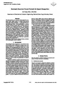
B. Elman Recurrent Neural Network The functionality of the recurrent network is determined by specifying the choice of network architecture, that is, the number and type of neurons, the location of feedback loops and the development of a suitable training algorithm. The Elman network was achieved with a configuration of two hidden layers, each having 10 tansigmoid neurons and one output layer with linear neuron. The algorithm achieved a very good meansquared error of 0.00058 with 100 numbers of training passes. The main mode of the system, as found from the MLP-NN predicted output was at 0.375 Hz which is very close to the actual vibration mode of the TRMS obtained through experimental tests. Comparing these with the corresponding results of MLP-NN modelling reveals that the results with Elman NN were far better than those with the MLP-NN. Performances of both NNs are shown in Figs. 6 and 7.
V.
CONCLUSION
Two types of ANNs, namely MLP NN and Elman RNN have been trained with the experimental data to characterise the dynamic behaviour of the TRMS. A 1 DOF vertical plane TRMS model, the dynamics of which resembles that of a helicopter, has been identified successfully. The extracted model has predicted the system behaviour well. Both the identified models have been verified on a real system with quite similar and accurate results.
time, Vv (t − 1) , voltage of main rotor at 2 previous sample times, Vv (t − 2) , pitch angle of the beam at previous time,
α v (t − 1) , pitch angle of the beam at 2 previous sample times, α v (t − 2) . The activation function for the hidden and output layers are logarithmic tansigmoid and linear respectively. The algorithm achieved a very good meansquared error of 0.0017 with 100 number training passes. The main mode of the system, as found from the MLP-NN predicted output is at 0.386 Hz which is very close to the actual vibration mode of the TRMS obtained through experimental test.
Authorized licensed use limited to: Sheffield University. Downloaded on July 15, 2009 at 09:44 from IEEE Xplore. Restrictions apply.
(a) Actual and predicted output
(a) Actual and predicted output
1
1
Actual output Elman predicted output
Actual output MLP-NN predicted output
0.5
Magnitude
Magnitude
0.5
0
0
-0.5
-0.5
0
100
200
300
400 500 600 Time(samples)
700
800
900
1000
200
300
400 500 600 Time(samples)
900
1000
0.6 0.4
0.4
0.2
Magnitude
0.2 0
0 -0.2
-0.2 -0.4
-0.4
-0.6
-0.6
-0.8
-0.8 -1 0
100
200
300
400 500 600 Time(samples)
700
800
900
1000
c) Spectral density of the output
2
0
100
200
300
400 500 600 Time(samples)
800
900
1000
10 Actual MLPNN prediction
Actual ElmanRNN prediction
1
1
10
10
0
0
Magnitude
10
-1
10
-2
10
-1
10
-2
10
10
-3
10
700
c) Spectral density of the output
2
10
Magnitude
800
0.8
0.6
-3
0
0.5
1
1.5
2 2.5 3 Frequency (Hz)
3.5
4
4.5
10
5
0
0.5
1
(d) Autocorrelation of the Prediction Error
2 2.5 3 Frequency (Hz)
3.5
4
4.5
600
800
5
1
0.8
0.8
0.6
0.6 0.4
0.2
0.2 Value
0.4
0
0
-0.2
-0.2
-0.4
-0.4
-0.6
-0.6
-0.8
-0.8
-1
1.5
(d) Autocorrelation of the Prediction Error
1
Value
700
1
0.8
Magnitude
100
(b) Error between actual and predicted output
(b) Error between actual and predicted output 1
-1
0
-800
-600
-400
-200
0 Lags
200
400
600
800
Figure 6. Twin rotor system using MLPNN prediction
-1
-800
-600
-400
-200
0 Lags
200
400
Figure 7. Twin rotor system using Elman NN prediction
Authorized licensed use limited to: Sheffield University. Downloaded on July 15, 2009 at 09:44 from IEEE Xplore. Restrictions apply.
REFERENCES [1] [2] [3]
[4]
[5] [6] [7] [8] [9] [10] [11] [12]
[13] [14] [15] [16] [17] [18] [19]
[20] [21] [22] [23]
Hornik, K., Stinchombe, M. and White, H., “Multilayer feedforward networks are universal approximators”, Neural Networks, 2, 1989, pp 359-366. Ljung, L. and Sjöberg, J., “A system identification on neural networks”, Proceedings of the IEEE Conference on Neural Networks for Signal Processing ll, Copenhagen, 1992, pp 423-435. Ahmad, S. M., Chipperfield, A. J., and Tokhi, M. O. “Dynamic modelling and linear quadratic Gaussian control of a twin rotor MIMO system”. Journal of Systems and Control Engineering, 1 (217), 2003, pp 203-227. Aldebrez, F. M., Mat Darus, I. Z., Tokhi, M. O., “Dynamic modelling of a twin rotor system in hovering position”, First International Symposium on Control, Communications and Signal Processing, Hammamet, Tunisia, 21-24 March, 2004. Rahideh, A., Shaheed, M. H. and Huijberts, H. J. C., “Dynamic modelling of a TRMS using analytical and empirical approaches”, Control Engineering Practise, 3 (16) 2008, pp 241-259. A. K. Jain and K. M. Mohiuddin, “Artificial Neural Networks: A Tutorial,” Computer: The IEEE Computer Society Magazine, 29 (3), 1996, pp 31-44. Jang, J.S., Sun, C. and Mizutani, E. (1997). Neuro fuzzy and soft computing, Prentice Hall, Upper Saddle River, NJ. Hinton, G. E. (1992) How neural networks learn from experience, Scientific American, 267 (3), September 1992, pp. 145-151 Rumelhart, D. E., Hinton, G. E., Williams, R. J. (1986) Learning representations by backpropagation errors, Nature, 323, pp. 533-536 Beale, R. and Jackson, T. (1992) Neural computing an introduction, Bristol, UK.: Institute Physics Hagan, M. T. and Menhaj, M. B., “Training feedforward networks with the Marquardt algorithm”, IEEE Transaction on Neural Networks, 5(6), 1994, pp 989-993. Al Seyab, R. K. and Cao, Y. (2008a) Nonlinear system identification for predictive control using continuous time recurrent neural networks and automatic differentiation, Journal of Process Control, 18 (6), July 2008, pp. 568-581 Draye, J., Pavisic, D., Libert, G. (1996) Dynamic recurrent neural networks: a dynamical analysis, IEEE Transactions on Systems, Man and Cybernetics, part B, 26 (5), pp. 692-706 Kosmatoupoulos, E., Polycarpou, M., Iannou, A. (1995) High-order neural network structures for identification of dynamical systems, IEEE Transactions on Neural Network, 6 (2), pp. 422-431 Kumpati, S., Narenda, F., Parthasarathy, K. (1990) Identification and control of dynamical systems using neural networks, IEEE Transactions of Neural Network, 1 (1), pp. 4-24 Parlos, A., Chong, K., Atiya, A. (1994) Application of the recurrent multi-layer perceptron in modelling complex process dynamics, IEEE Transactions on Neural Network, 5 (2), pp. 255-266 Ren, X. M., Rad, A. B., Chan, P. T., Lun Lo, W. (2003) Identification and control of continuous-time nonlinear systems via dynamic neural networks, IEEE Transactions Industrial Electron, 50 (3), pp. 478-786 Sio, K. C. and Lee, C. K. (1996) Identification of a nonlinear system with neural networks, Proceedings of the Advance Motion Control’96, MIE Japan, pp. 287-292 Su, H. T. and McAvoy, T. J. (1997) Artificial neural networks for nonlinear process identification and control, In Editors: Henson, M. A., Seborg, D. E. (Eds.), Nonlinear Process Control, Prentice-Hall, New Jersey, pp. 371-428 Al Seyab, R. K. and Cao, Y. (2008b) Differential recurrent neural network based predictive control, Journal of Computers and Chemical Engineering, 32, pp. 1533-1545 Funahashi, K. L. and Nakamura, Y. (1993) Approximation of dynamical systems by continuous time recurrent neural networks, Neural Networks, 6, pp. 183-192 Jin, L., Nikiforuk, P., Gupta, M. (1995) Approximation of discrete-time state-space trajectories using dynamic recurrent neural networks, IEEE Transactions on Automatic Control, 40 (7), pp. 1266-1270 Delgado, A., Kambhampati, C., Warwick, K. (1995) Dynamic recurrent neural network for system identification and control, IEE Proceedings on Control Theory Applications, 124 (4), pp. 307-314
[24] Hush, D. R., Horne, B. G. (1993) Progress in supervised neural networks, IEEE Signal Processing Magazine, 1, pp 8-39 [25] Haykin, S. (1999) Neural Networks: a comprehensive foundation, Second Edition, Prentice Hall, Upper saddle River, NJ, 1999, pp. 20-21 [26] Linkens, D and Nyongesa, Y., “Learning systems in intelligent control: an appraisal of fuzzy, neural and genetic algorithm control applications”, IEE Proceedings of Control Theory and Applications, 134(4), 1996, pp 367-385. [27] Elman, J., “Finding structure in time”, Cognitive Science, 14, 1990, pp179-211. [28] Moody, J. and Darken, C., “Fast learning in networks of locally-tuned processing units”, Neural Computation, 1, 1989, pp 281-294. [29] Demuth, H., Beale, M. and Hagan, M., Neural Network Toolbox 6.0 User’s Guide, The Mathworks, (2008). [30] Sastry, P. S., Santharam, G. and Unnikrishnan, K. P., “ Memory neural networks for identification and dynamic systems”,IEEE transactions on Neural Networks, 5(2), 1994, pp 306-319. [31] Billings, S. A. and Voon, W. S. N., (1986). Correlation based model validity test for non-linear models. International Journal of Control, 44 (1), pp 235-244. [32] Billings, S. A. and Zhu, Q. M., (1994). Nonlinear model validation using correlation tests. International Journal of Control, 60 (6), pp 11071120.
Authorized licensed use limited to: Sheffield University. Downloaded on July 15, 2009 at 09:44 from IEEE Xplore. Restrictions apply.