Model-based processing scheme for quantitative 4-d cardiac mri ...

IEEE TRANSACTIONS ON INFORMATION TECHNOLOGY IN BIOMEDICINE, VOL. 6, NO. 1, MARCH 2002

59

Model-Based Processing Scheme for Quantitative 4-D Cardiac MRI Analysis George Stalidis, Nicos Maglaveras, Member, IEEE, Serafim N. Efstratiadis, Member, IEEE, Athanasios S. Dimitriadis, and Costas Pappas, Member, IEEE

Abstract—In this paper, we present an integrated model-based processing scheme for cardiac magnetic resonance imaging (MRI), embedded in an interactive computing environment suitable for quantitative cardiac analysis, which provides a set of functions for the extraction, modeling, and visualization of cardiac shape and deformation. The methods apply four-dimensional (4-D) processing (three spatial and one temporal) to multiphase multislice MRI acquisitions and produce a continuous 4-D model of the myocardial surface deformation. The model is used to measure diagnostically useful parameters, such as wall motion, myocardial thicking, and myocardial mass measurements. The proposed model-based shape extraction method has the advantage of integrating local information into an overall representation and produces a robust description of cardiac cavities. A learning segmentation process that incorporates a generating-shrinking neural network is combined with a spatiotemporal parametric modeling method through functional basis decomposition. A multiscale approach is adopted, which uses at each step a coarse-scale model defined at the previous step in order to constrain the boundary detection. The representation accuracy starts from a coarse but smooth estimation of the approximate cardiac shape and is gradually increased to the desired detail. The main advantages of the proposed methods are efficiency, lack of uncertainty about convergence, and robustness to image artifacts. Experimental results obtained from application to clinical multislice multiphase MRI examinations of normal volunteers and patients with medical record of myocardial infarction were satisfactory in terms of accuracy and robustness. Index Terms—Cardiac analysis, deformable representation, multiphase magnetic resonance imaging (MRI), parametric modeling, shape extraction.

I. INTRODUCTION

I

N THE last decade, the growing use of the magnetic resonance imaging (MRI) modality to cardiac diagnosis is mainly due to its noninvasive operation, excellent tissue contrast, and spatial resolution in three dimensions (3-D). Apart from multislice acquisitions, multiphase electrocardioManuscript received February 2, 2000; revised November 5, 2001. This work was supported in part by the Greek Secretariat of Research and Technology, Ministry of Industry and Development, under the IPER-266 program and in part by the European Commission under the Integration and Communication for the Continuity of Cardiac Care (I4C) project. G. Stalidis, N. Maglaveras, and C. Pappas are with the Lab of Medical Informatics, The Medical School, Aristotle University, 54006 Thessaloniki, Greece (e-mail: [email protected]; [email protected]; [email protected]). S. N. Efstratiadis is with the Lab of Medical Informatics, The Medical School, Aristotle University, 54006 Thessaloniki, Greece, and the Department of Electronics, Technological Education Institute, 54639 Thessaloniki, Greece (e-mail: [email protected]). A. S. Dimitriadis is with AHEPA General Hospital, Department of Radiology, The Medical School, Aristotle University, 54006 Thessaloniki, Greece. Publisher Item Identifier S 1089-7771(02)02013-7.

gram (ECG)-gated acquisitions offer valuable information on the cardiac motion with good resolution. The geometrical and functional value of this information requires processing methods that make use of the MRI multidimensional nature and are not restricted to two-dimensional (2-D) processing. A complete representation of cardiac chambers is provided by a four-dimensional (4-D) cardiac model. Such a model provides valuable diagnostic information for both visualization [1], [2] and quantitative evaluation of useful parameters, such as regional wall thickness, curvature, and their dynamics [3]–[6]. A number of techniques have been reported in the literature making use of mathematical models for detection and representation of organ boundaries in medical images. Reference [7] used a Fourier parametrically deformable model in order to detect object boundaries in 2-D images and then applied the method to cardiac MRI. While this model is in principle similar to that presented here, the difference lies in the model-fitting approach to the image data, which uses optimization in the parameter space based on their probability distribution. Similar Fourier descriptors were presented in [8]. In previous reports [9]–[11], active contour models were used to determine borders of structures. These models are attracted by external forces determined by the image data. An extension of the active contours to 3-D surface models is the 3-D balloon model reported in [12], which has been applied to the detection of the left ventricular chamber in cardiac MRI data. Graph search and dynamic programming methods that minimize an overall path cost function were also reported in [13]–[16]. Recently, Niessen et al. [17] presented a modification to the geodesic deformable model and applied it to the segmentation of cardiac computed tomography and MRI. The study of cardiac motion using geometrical models has been proposed by several researchers. In [1], the presented deformable model approximates the left ventricle using a few parameters corresponding to physical properties, which vary locally as functions of position. The model is fit using forces exerted by detected points derived from magnetically tagged data (MRI-SPAMM). Thomas et al. [18] adopted a multidimensional stochastic model containing prior functional information and used tagged MRI data for estimating the displacement field of the moving myocardium. A different approach [2] combined surface construction using minimal area triangulation of segmented MRI based on the Bezier tensor product. The left ventricular motion was also studied in [19] using optical flow methods. Point-to-point myocardial registration between different phases, without magnetic tagging in 2-D image sequences [20] and 4-D images [21], was addressed using geometrical surface characteristics (e.g., curvature). Recently, a

1089-7771/02$17.00 © 2002 IEEE

60


curvature-based approach was adopted for studying shape deformation characteristics of cardiac motion [22]. The latter was also studied for diagnostic purposes by employing multimodal image processing techniques and 3-D volume rendering implemented on a single-instruction multiple-data parallel machine, achieving real-time processing and visualization [23]. In this paper, we present an integrated processing scheme for cardiac MRI, embedded in an interactive computing environment suitable for quantitative cardiac analysis. The proposed scheme provides a set of functions for the extraction, modeling, and visualization of cardiac geometrical shape and deformation. The methods apply 4-D processing (three spatial and one temporal) to multiphase multislice MRI acquisitions and produce a continuous 4-D model of the myocardial surface deformation. The use of deformable models for studying the cardiac shape and motion, in contrast to directly applying measurement algorithms to the data, is justified as follows. First, deformable modeling is a powerful tool for discriminating objects from their surroundings due to the integration of incomplete local information derived from properties, such as pixel intensity, edge strength, and texture, into an overall shape description. In this way, a robust object representation is produced, a property particularly important in medical images, where discontinuities in shape are often caused by low contrast, artifacts, and noise. Second, the adopted approach is more general since many measurement types can be readily obtained based on the mathematical object description, allowing further enhancement of the analysis. In addition, the model is useful for visualization and distributed processing purposes. The proposed model-based shape extraction method produces a robust description of cardiac cavities used to measure diagnostically useful parameters, such as wall motion, myocardial thicking, and myocardial mass measurements. The detection of myocardial borders was based on a segmentation process with learning features, which incorporated a neural network classifier with generating-shrinking capabilities [33]. The classifier was combined with a boundary detection method, which models cardiac cavities with parametric functions and then applies decomposition to a Fourier or wavelet functional basis. A multiscale approach is adopted, which uses at each step a coarse-scale model defined at the previous step in order to constrain the boundary detection. The representation accuracy starts from a coarse but smooth estimation of the approximate cardiac shape and is gradually increased to the desired detail. This approach results in improved efficiency, lack of uncertainty about convergence, and robustness to image artifacts. An important characteristic of the proposed scheme is its enhanced interactivity with the user. However, the required guidance regarding representative point locations of the different classes in the MRI is minimal due to the learning classifier, which allows the automated operation based on certain initial assumptions. If the modeling progress is not satisfactory, the user can provide additional guidance in order to correct the process. The proposed algorithm was successfully applied to a large number of multislice multiphase MRI data sets, obtained with conventional protocols. In the following, the modeling approach for representing the extracted information is presented in Section II. The methods used by the cardiac analysis system, including preprocessing,

segmentation, model fitting, and measurement, are described in Section III. Experimental results and their evaluation by clinicians are given in Section IV. Conclusions are discussed in Section V. II. CARDIAC INFORMATION REPRESENTATION A. Parametric Representation The choice of the representative functional formulation of the cardiac information is important for cardiac analysis. In our work, the cardiac surface is represented by a deformable parametric model, which employs decomposition to basis functions. The spatial coordinates of the surface points are represented by , , and . three real functions: The free parameters , , and provide the three degrees of freedom required and are conveniently selected to correspond to specific directions for a straightforward reconstruction. More specifically, if one considers a cylindrical shape for the ventricular myocardial surface, is assigned to the circular direction around the cylinder, to the longitudinal direction from top to bottom, and to the temporal direction. The functions repreundergo an appropriate senting the cardiac surface transformation by decomposition to a set of multidimensional basis functions. A selected set of the resulting coefficients forms the model parameters. The two decomposition approaches considered are the Fourier and wavelet transforms. The Fourier decomposition approach, also used in computer graphics, represents shapes by their Fourier descriptors [8] and is analogous to storage of coordinate values by their harmonic content rather than their spatial position. Coarse shape characteristics are captured by low-order harmonics, while higher order harmonics represent increasing detail. Expanding this idea to deforming shapes by adding the temporal dimension, cardiac surfaces are modeled by their predominant spatiotemporal frequency components instead of position information. The reconstruction of the cardiac surface is continuous based on the interpolation properties of the trigonometric basis functions. The wavelet-based representation is similar to the Fourier-based one since it uses the same set of parametric functions to represent the deforming surface. However, these functions are decomposed into a multidimensional wavelet basis instead of a trigonometric basis. While Fourier transform coefficients express the shape frequency content, the wavelet transform coefficients express the shape detail content, defined as the additional information needed to produce a higher resolution representation from a lower one. The motivation behind the use of wavelets lies on their ability to provide a multiresolution representation of the signal local properties. This is particularly desirable in applications where increased accuracy is required in certain areas of interest. Note that the model parameters using Fourier or wavelet transform do not correspond to any physical property of the surface, such as size, rotation, or curvature, apart from the zero-order coefficients that correspond to global translation. B. Deformable Modeling The above model is fit to the examination data using a number of surface points extracted from the images. The model parameters are estimated using the surface point coordinates as samples

STALIDIS et al.: MODEL-BASED PROCESSING SCHEME FOR QUANTITATIVE 4-D CARDIAC MRI ANALYSIS

of the original functions. The number of samples considered is restricted by the size of the original data set, with the greatest restriction in the temporal resolution, since the number of phases in multiphase MRI is usually 16 (35 ms time step) or smaller. In 2-D multislice acquisitions, the interslice distance (usually 4 mm or larger) also limits the number of samples in the vertical dimension. On the other hand, the intraslice image resolution is typically adequate. The size of the parameter set is reduced by rejecting the least important coefficients while ensuring a satisfactory level of representation accuracy. The rejection of coefficients reduces the effect of detail and controls the smoothness of the resulting cardiac surface according to the quality of the original data. In the case of good-quality high-resolution data, accuracy can be increased. However, for noisy low-resolution or low-contrast original data, a low approximation order should be selected so that the resulting model is robust to noise and represents the overall organ shape as reliably as possible. The final number of model coefficients, which defines the model order or complexity, depends on the above selections. For example, a typical choice of eight in all dimensions results in 2048 floating-point coefficients per 4-D deformable surface. Considering that these coefficients fully describe a continuously deformable 3-D surface with all the required anatomical detail, they form a quite compact representation of the cardiac information when compared to the original 4-D data size. The optimal model order is derived experimentally by studying the mean error of the final representation and the modeling performance. This procedure was carried out with the help of a radiologist by manually tracing the endocardial and epicardial contours in three 4-D data sets. The resulting data were then used as a reference surface for error measurements. The deformable model considers an appropriate ordering and assignment mode of the available surface points into a set of 3-D transformation matrices. The model properties are determined by the ordering and assignment mode (Section III-E), as well as the underlying adopted transform. Regarding the adopted transform, the Fourier and wavelet approaches have different properties that make each one of them suitable to application cases with different requirements. While the wavelet-based model allows the preservation of local detail even at low model orders, the Fourier-based model allows the preservation of the overall shape and smooths out detail uniformly over the entire range. Although, the Fourier transform is applied directly to the original data, the wavelet decomposition is implemented in a hierarchical fashion by convolving successive approximations of the initial function with the appropriate quadrature mirror filters. The surface reconstruction is performed by the inverse transform, which may be implemented hierarchically using the corresponding inverse filter. The reconstruction quality depends on the interpolation properties of the corresponding basis functions. The Daubechies class of wavelets was used in our work, offering a large scale of functions from very localized in space to very smooth. Their important characteristic is separability resulting in great computational efficiency when applied to multidimensional data. An acceptable compromise between localization and smoothness is provided by the sixth-order Daubechies filters (DAUB6). The described deformable modeling was implemented in an interactive computing scheme (Section III),

61

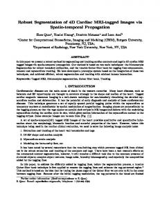
where the two transforms are used according to their inherent properties for best results. III. MODEL-BASED MRI PROCESSING AND ANALYSIS A. Method Outline The problem in question is the accurate and robust extraction of the endocardial and epicardial surfaces of cardiac cavities from MRI data. Their shape and deformation is then modeled to be used for measuring quantities of diagnostic value. Particular focus is placed on the left ventricle, which is clinically most important. However, the proposed method may be applied with no restriction to other cavities, after certain necessary adjustments related to different expected size and shape complexity are made. We consider a 4-D model that is smooth and continuous in both space and time, thus allowing the measurement of myocardial surface motion. Cardiac motion is quite complicated since it involves translation, rotation, and, most important, deformation. Therefore, its study in two dimensions is rather inadequate since the same slice image in different phases does not usually correspond to the same tissue. The proposed method is applied to multislice multiphase MR images or 3-D multiphase data acquired by either bright blood or dark blood conventional protocols. In Fig. 1, a block diagram depicts the flow of the proposed method. A multiscale fitting process is followed, where in each step the rough version of the model produced by the previous step is used in deriving a more detailed model. The procedure is initiated by the user, who indicates the rough position of the cavity, as well as reference samples of myocardium, blood, and lung. The size of a predefined coarse cardiac surface model is set according to the user input and is used as an initial reference by the subsequent stages of the algorithm. The sensitive task of discriminating the tissue type is handled by a trained neural network (NN)-based classifier. Initial training is performed with minimal user guidance and can be improved (if necessary) by user interaction. The classifier output, the coarse model, and the image intensity gradient are combined by a radial search algorithm, which identifies endocardial and epicardial points at a finer scale. Then, the model fitting task is performed by inserting lexicographically the coordinates of the detected points in 3-D matrices and by calculating the model parameters using an appropriate transform. The resulting model is used to guide the detection and model-fitting process at a higher scale, until the required accuracy level is reached. The above iterative method requires a fairly small number of steps (typically three or four ) and relatively low computational cost. As a result, the method is efficient and considerably faster than alternative techniques reported in the literature, such as optimization methods and graph searching. B. Image Preprocessing Stage Initially, the acquired 4-D MRI data, using conventional MR equipment and protocols, are transferred from the MR unit to a graphics workstation for processing. Modern MR systems produce images with resolution from 80 80 to 256 256 and a number of 20 or more locations, or isotropic 3-D data with resolution of the same order in all three spatial dimensions. This spatial resolution is considered adequate for our application. The

62


a slice-by-slice basis, which is the default way of viewing raw multislice data, the user is viewing sections of 3-D data. Since the resolution of volume data, which defines the number of planes available, is much larger than the number of slices available at multislice acquisitions, the user is also given the possibility to skip unnecessary planes of the 3-D data by selecting an intersection distance. In addition to the above position information, an approximate small set of samples from the myocardium, blood (intracavity), and surrounding regions needs to be indicated by the operator in order to be used in the segmentation phase described below. C. Classification-Based Segmentation

Fig. 1.

Method outline.

number of temporal phases ranges from six to 24 per cardiac cycle, corresponding to a minimum time step of 20 ms. As a first step of the modeling method, the user visualizes the data and determines the approximate position of the left ventricle using a mouse-driven interface. In the case of 2-D multislice data, for each phase, the user selects the slice closest to the cavity base and the one closest to the cavity apex, assuming axial acquisition. Then, the cavity center in both slice images, identifying the approximate centroid, is indicated. The line connecting the two selected points roughly defines the long axis of the ventricle and is used as reference for its size and orientation. In practice, we found that the above procedure alone is sufficient to indicate the long axis at diastole and systole and does not need to be repeated for each phase. Note that accurate selection of the above centroids and exact definition of the ventricle long axis is not necessary and does not affect the performance of the method. In the case of 3-D data, a similar procedure is performed by the user for selecting sections of the volume data instead of slices. User interaction with 3-D data is very similar to the 2-D multislice case. Instead of viewing images on

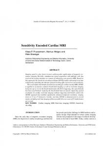
The extraction of the cardiac surfaces requires the segmentation of the MRI data into myocardium, intracavity region (blood), and the cavity surrounding area based on the pixel intensity values, since MRI typically retains good contrast among myocardium, blood, lung, and fat. The large number of suitable segmentation approaches in the literature, particularly applied to cardiac MRI, employ, among other techniques, statistical analysis, multiresolution, and fuzzy methods or NNs [29]–[32]. More recently, the cardiac ventricle boundaries were defined by refining the segmentation threshold according to a learning algorithm [28]. In our method, we adopt an efficient NN-based classifier [33] that was successfully applied to ECG signal processing [34]. The proposed segmentation network is trained on a small number of representative tissue points and is used to segment image points into three classes: lung, myocardium, and blood. In selecting the above classifier, we considered its efficiency when compared to alternative, more computationally intensive techniques, which are prohibitive to use in practice due to the large size of typical 4-D data sets. The generating-shrinking neural network classifier (GSNNC), shown in Fig. 2, is based on supervised feedforward NNs and generates a three-layer network to classify random patterns in [33]. This approach is the -dimensional Euclidean space preferred over the backpropagation algorithm because 1) it can separate the training patterns very fast (about 1000 times faster than backpropagation); 2) its behavior is analytically described; and 3) the learning of a new pattern does not induce loss of previous training (on-line training). More specifically, let us consider the problem of separating number of classes and a three-NN-layer architecture. The first (input) layer receives information from an -dimensional vector, which is the input pattern. Given a reference constant , an ( 1)-dimensional vector is formed. The input layer has as many neurons as the trained patterns and its output is for

(1)

is the weight of the connection between the th input where component and the th neuron, is the -dimensional vector, and is the total number of training patterns. The secondlayer neurons receive input only from the input layer and form the following output: for

(2)


63

large intraslice intensity variations around the myocardium, surrounding area, or blood. In our approach, the NN classifier took advantage of the rather consistent behavior of this artifact over a significant number of successive slices and used position information to create appropriate decision regions that took into account the intensity gradients. Specifically, we concluded to a three-dimensional input pattern, consisting of 1) pixel intensity (range 0 to 255); 2) position in the image, measured as angle around the centroid of the cavity (range 0 to 359); 3) slice location (range 0 to 35).

Fig. 2. The generating-shrinking neural network classifier.

where (3) The third layer consists of mined by

neurons and its output is deter-

for

(4)

is the weight of the to connection. Finally, the where and are defined as follows: weighting factors for for

(5)

for if is the class for pattern otherwise

for (6)

The processing of input vectors by the NN actually involves normalization of magnitude [see (5)], which could lead to an extremely scattered decision region, depending on the input values. For this reason, the constant is used as an additional element in the input vector, ensuring a minimum vector magnitude. As a consequence, the morphology of the decision region is dependent on the value of . The connection between the constant and the performance of the classifier is mentioned in [33]. It is worth noting that the sensitivity of the performance on the exact value is very small, due to the learning feature of the NN. It can thus be safely selected to be comparable (same order of magnitude) with the mean of the other input elements. The GSNNC algorithm is trained by input patterns using its on-line feature. The NN input is in general a set of statistical indexes associated with the image intensity, texture, and structure around each pixel. Clearly, the consideration of several parameters allows a more robust clustering. On the other hand, an unnecessary increase of input pattern dimension enlarges the computational requirements. The dimension of the input vector thus results from the number of input values that play a useful role in the intended classification. In our case, pixel intensity alone was sufficient for tissue discrimination due to the good MRI contrast between tissue types. However, the NN input pattern also needed to include position information in order to deal with the standard problem of intensity gradients. This artifact involves considerable changes in the intensity scale, such as interslice differences or possible

Including the temporal phase as an additional parameter did not result in any significant improvement, for the data we used may be a straightforward modification in the case of data with interphase intensity gradients. NN training is performed on-line, simultaneously with the input pattern selection stage by the user. This means that whenever the user selects a new training pattern through the graphical interface, the corresponding node is created in the second NN layer and the weight matrices are updated. This process is computationally very fast and practically carried out instantaneously before the next training pattern is selected. Moreover, it is possible to provide additional training patterns at any time without discarding the previous training. This property allows the interactive design of the method, including possible corrective intervention by the user. The classification process may start with minimal user guidance, e.g., one point from each class. Alternatively, a fully automated method for identifying an initial pattern per class can be used. We introduce a hard rule, which derives training patterns for class using the histogram of one reprefor sentative image, such as predefined bounds the intensity values. Although this provided satisfactory initial segmentation results in most cases, it is not guaranteed to work in a wide range of MRI data sets. Thus, successful unsupervised NN training requires prior information of the cardiac structure and texture by developing a knowledge base used for selecting good initial training sets and bound values (intelligent training). The success of the method improves with its extended clinical use on sufficient number of different examination cases. User intervention may be necessary only in certain atypical cases, resulting in unsuccessful performance of the initial segmentation stage. Within this work, this was implemented in a preliminary form in order to save time during our experiments. An initial set of training samples, as they were selected by the user, gave satisfactory segmentation results without additional guidance. The set was used to form the “knowledge” regarding the selection of training samples. The set comprised 32 points, spread into different classes and slice locations in end diastole. From the intensity values of these points, a lookup table was formed with the mean intensity for each class. An automatic procedure was then implemented which scans of eight slices in end diastole to find one sample point from each class in each slice (24 points in total). The criteria for selecting these points are to have intensity close to the corresponding value in the lookup table and to belong in a uniform region with similar intensities and size of at least 5 5 pixels. It is noted that the technique in this form was only

64


(a)

(b)

(c)

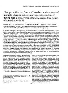
Fig. 3. Application of the GSNNC algorithm for segmenting an axial systolic slice. (a) Original image. (b) Segmented image using automatically derived training patterns. (c) Segmented image using additional training pattern for myocardium. Segmentation labeling: blood (white), myocardium (gray), lung (black).

a crude approach toward intelligent training. However, it was found useful in practice in terms of saving user interaction time and depicted the advantage of the segmentation method to allow progressive training. Given the training input, the GSNNC reduces its size by rejecting nodes, according to a certain shrinking rule, and classifies input patterns representing image points and their properties into myocardium, blood, or lung. Due to the GSNNC shrinking property and feed-forward structure, its output is calculated very efficiently. In case of unsatisfactory results, the user may select additional training points, indicating the desirable behavior of the classifier at the dubious locations or phases at a negligible additional computational cost. User intervention is possible through a graphical interface, which allows the viewing of slice-by-slice segmentation results in parallel with the original data and the selection of additional training samples. The user is able to view selected segmentation results and to decide if he wants to intervene in the training before or after the execution of the boundary detection algorithm. It is also possible to ask for the automatic selection of an initial training set or to reset the training process. In a typical examination, the number of neurons created in the second layer is on the order of 20 to 100. The number of nodes rejected by the shrinking property can be minimum (e.g., one or two nodes) when the number of samples is small, and a reduction to half can be reached when the samples contain significant redundancy. Finally, a nonlinear filtering operation, based on the majority of labels within a window, is applied to the segmented image in order to filter out very small isolated regions attributed to noise. of Specifically, for each pixel , given a rectangular window centered around pixel , we have size if

is in class

otherwise

(7)

For each class , we have (8) (9)

If

and pixel is classified to class and , then pixel is classified to the majority class , . In other words, the above filter which corresponds to computes the majority of the labels within a specified rectangular window around the working point. If this point is labeled differently than the majority and the number of all points in the window with different labels than the majority is smaller than a predetermined threshold, then the center point is changed to the majority class. This threshold and the filter support size are selected so that the filter has maximal effect only on small regions that are attributed to noise and produces minimal (almost zero) undesirable distortion to the tissue boundaries. The best results were obtained for a 5 5 size window and a threshold value equal to four. Fig. 3(b) and (c) shows the GSNNC segmentation results with no user guidance and with an additional training pattern for the myocardium, respectively, when applied to the axial systolic slice of Fig. 3(a). Note the drastic improvement in the GSNNC output quality in Fig. 3(c). D. Endocardial–Epicardial Border Detection The output of the classification algorithm, along with a coarse reference 4-D surface model and the image intensity gradient, are considered in the identification of the endocardial and epicardial boundary points. This operation is performed slice-by-slice over the entire 4-D set. In the case of 3-D data sets, 2-D slice images are used instead of 3-D image sections. The search is initiated from the user-defined points, which approximately determine the location and orientation of the left ventricle. These points are used to derive the approximate centroid of the left ventricle cavity for each location and phase using linear interpolation in space and time. More specifically, the border detection method consists of the following steps. Step 1) Using the cavity centroid as the starting point, a search for endocardial boundary points is conducted radially on each slice image, as shown in Fig. 4. The angle step is set according to the required number of samples and the radius is constrained to a maximum value .


65

Finally, is an approximation of the image derivative along the search direction, calculated by a Gaussian convolution filter of small scale, that is (14)

Fig. 4. Epicardial boundary radial search process. Note that the erroneous initial detections (upper part of the slice), due to the confusion between left and right ventricular muscle, are subsequently corrected by the multiscale surface fitting procedure.

Step 2) For all scanned points , , along the radius, a strength value , representing the probability that the point is the endocardial boundary, is evaluated as described below. Step 3) The maximum strength point is selected as a boundary point and its coordinates are stored. Step 4) If the cycle is not completed, go to Step 2) in order to detect the boundary point at the next angle step along the radius, starting again from the center. Step 5) When the cycle is completed, the algorithm proceeds to a subsequent slice, until the entire volume of the cavity of interest is covered for all phases. of pixel , used for selecting the The strength value boundary point at the current radius, is a weighted sum of three . These terms are related to the output of terms , the classification algorithm ( ), the reference coarse scale model ( ), and the image gradient ( ), respectively. More specifically (10) is defined for each pixel

as (11)

where

is the GSNNC output defined as if is classified as myocardium

(12) if is classified as blood. is related to the solution deviation from the coarser scale model and is evaluated as the squared distance between pixel and the model boundary estimate at the specific angle step , that is (13)

is the Gaussian derivative filter and the image where intensity in a 1-D window along the radius centered at . The decision on defining the boundary is equivalent to finding are the point with maximum strength value. The weights selected with the goal of obtaining the optimal decision. Each determines the influence of the corresponding factor to the and take positive values, is negfinal result. While ative since the deviation from the prior model should act as a discouraging factor. Note that the weighted computation of suggests that the final decision on the boundary is not based only on the classification algorithm. The latter produces erroneous results in certain cases when the myocardium boundary is not detectable (not even visible by the clinician). In such cases, the coarse model takes over and attracts the solution to a reasonable approximation. The precision of this solution is assisted by strong intensity gradients in the original image. All three terms are computed quite efficiently and provide effective information to the boundary detection process. Their use is complementary since they combine learning-based and location-dependent classification, prior knowledge, and local inforwere evaluated by optimization of the mation. The weights algorithm performance on a large number of typical data sets using the root mean squared (rms) error between the detected points and manually traced points as a cost function and a gra, dient descent algorithm. The resulting weight values ( , ) gave the smallest detection error and were used throughout all the experiments. It is noted that the above values incorporate a normalization factor for the terms , since the latter were of a different range. After the cycle is completed for the endocardium, the epicardial boundary points are detected by applying a similar procedure. In this case, the transition is not always directed from myocardium to blood, as in the endocardium. The tissue of the outer side of the epicardial surface can be lung, epicardial fat, right ventricular myocardium, or right ventricular blood. These tissues can be of higher, smaller or similar image intensity. The search begins from the endocardial boundary, instead of the centroid, using the previously defined endocardial model. Thus, the boundary detection algorithm is adjusted to detect transition either from myocardium to blood or from myocardium to lung. On the other hand, transition from left ventricular to right ventricular myocardium is not detectable, and estimation must rely entirely on model-based interpolation. The fact that the detection of the epicardium depends on the endocardial model did not cause problems of error accumulation in practice. The performance of detecting the epicardium has been found to be in general better when using the endocardium position than when ignoring it. The nature of the dependence between the two procedures is such that the information of the endocardial boundary gives a better starting point for the search of the epicardium position. The exact location, however, is defined by the iterative algorithm, which is based on local information and the classification result. Thus its detection is not sensitive to small errors

66


Fig. 5. (a) Slice-by-slice tracing of boundary contours for each phase. (b) Lexicographically ordered storage of detected points in 3-D matrices.

that may occur in the detection of the endocardium position. An example of the algorithm performance and the detection errors that may occur is given in Fig. 4, where the white lines indicate the search path until a suitable boundary point is found. E. Model Parameter Estimation The model parameters are computed by applying a multidimensional transform to the data extracted by the boundary detection process. The coordinates of detected points are stored in 3-D matrices, one for each coordinate. Successive points sampled along a closed contour on the same plane are arranged in one matrix row; successive sections are arranged in successive rows; and consecutive phases are arranged with the same order in different matrix planes, as illustrated in Fig. 5. The number of samples in each dimension is kept constant for the entire data set. This sampling rate is selected for the final model according to the resolution of the original data. Then, the appropriate transform (Fourier or wavelet) is applied to all matrices, producing the raw model parameters. Their final number is determined by keeping either the lowest frequency Fourier coefficients (up to a predefined order) or the predominant Wavelet parameters by applying a thresholding operation on their magnitude. More specifically, the parameters of the Fourier-based model are calculated as follows. and , one for each Step 1) Define three 3-D matrices and , with dimensample point coordinate 2 , where and are sions 2 number of samples per slice, number of slices, and number of phases, respectively. Step 2) Store coordinates in the matrices as , , for , , . Similarly for and . Step 3) Create a mirror copy of the above values in each matrix with respect to the slice-phase plane. Step 4) Apply 3-D fast Fourier transform on each matrix. Step 5) Discard high-order coefficients above the specified orders of approximation. The wavelet-based model coefficients are produced following a similar procedure. and , one for each Step 1) Define three 3-D matrices and , with dimensample point coordinate , where and are number sions

of samples per slice, number of slices, and number of phases, respectively. Step 2) Store coordinates in the matrices as for , , . Similarly for and . Step 3) Apply 3-D wavelet transform on each matrix. Step 4) Apply threshold operation to discard coefficients with low magnitude. In order for the resulting free model parameters to be representative of a specific direction on the surface, a correspondence between the assigned position of the points in the transformation matrix and the corresponding region on the surface is required. However, it should be noted that in the temporal direction, the requirement was that points on a specific matrix row and column correspond in each matrix plane to the same tissue as it moves in different phases in order to achieve a consistent reconstruction regarding motion of specific regions. It is evident that the latter requires true functional data, which is not available to our algorithm. Consequently, the proposed model accurately represents the 3-D shape of the left ventricle at each instant without ensuring that the trajectory of any surface point along the temporal variable is the true motion of a specific tissue point. F. Quantitative Evaluation of Cardiac Function The model-based extraction method provides a quantitative representation of the myocardial surfaces and their deformation, based on which diagnostic parameters are derived. As an application of the parametric model, myocardial thickness and approximate strain are calculated and displayed. According to clinicians, myocardial strain is of high diagnostic value, since it can reveal abnormalities in myocardial contraction. The strain estimates are expressed as variations in longitudinal shortening, measured as a percentage of diastolic value. Abnormal myocardial strain is an indication of vulnerability to injury, in particular ischemia, arrhythmia, cell dropout, and aneurysm rupture. It is also related to the expected progression of disease, such as the infarct expansion, ventricular dilation, formation of aneurysm, and response to reperfusion. As reported in [35], strain measurements obtained with Doppler strain rate imaging have been shown to discriminate healthy tissue contracting normally from infarcted tissue. Studies on patients with acute myocardial infarction and healthy volunteers have shown a visible border


zone between ischemic and nonischemic tissue. Longitudinal strain (peak shortening) in normal left ventricular myocardium typically has negative values in the area of 10 to 14 (%), while infarcted areas are not contracting and give positive strain values. In our experiments, myocardial thickness was measured during the entire cardiac cycle and was used to estimate radial strain as the difference in thickness of a specific region between systole and diastole (measured as a percentage of full length). Myocardial thickness was measured using the following algorithm. Step 1) For a specific position along the long axis, the endocardial boundary at diastole is reconstructed as a curve on the plane vertical to the long axis that passes from this position. Step 2) For each boundary point on the curve, the direction normal to the surface is calculated, using a smoother reconstruction by further decreasing the model order. Step 3) The myocardial thickness is measured by searching the point at which the normal vector intersects the epicardial surface. Step 4) The resulting thickness value and the coordinates of the corresponding endocardial point are stored. Step 5) Steps 1) to 4) are iterated for successive positions on the long axis until the endocardial surface is covered. Step 6) Steps 1) to 5) are iterated at successive time instances until the entire cardiac cycle is covered. A set of thickness measurements is thus acquired for each temporal phase. The number of surface points to be measured is selectable by the user, according to the desirable resolution in the calculations. The produced values are color coded on the endocardial surface and displayed in CINE mode, together with the surface deformation. This view is suitable for qualitative evaluation of cardiac motion. Since it requires no registration, each phase is accurately displayed. Furthermore, thickness measurements are used to derive myocardial strain maps. Strain is estimated as the difference in thickness from diastole to systole, expressed as a percentage of diastolic value. The produced values are displayed as gray levels coded on the endocardial surface. The results are approximate, since there is no real functional information in the original data to accurately measure myocardial displacement. However, the provided accuracy was satisfactory for important diagnostic applications, such as detection of hypokinetic tissue. IV. CLINICAL APPLICATION AND RESULTS The proposed methods were applied to 2-D multislice multiphase and 3-D multiphase cardiac MRI data. In the case of 2-D data, the image size was 80 80 with a field of view 11.2 cm and interslice distance of 6 mm. The number of slices varied from 16 to 24 and the number of phases from 16 to 20 phases per location. The 2-D data were acquired with a 3.5-T system from three different patients. The images were axial, ECG gated, and T2 weighted. The 3-D acquisitions were also T2-weighted. The data size was 256 145 85 for each phase, and a total

67

Fig. 6. (a) Detected endocardial surfaces. (b) Detected epicardial surfaces. Phases (left) 1 and (right) 8 of total 16.

of six phases were available. A typical net execution time of the proposed algorithm was on the order of a few minutes executed on a Silicon Graphics INDIGO 4000 machine. This time interval included the boundary point detection and the construction of a deformable model for all steps of increasing accuracy, up to the final model scale. The entire process for each patient, including human interaction, lasted on average less than 10 min. To obtain a reference for evaluating the algorithm results, the original data were manually traced by an experienced radiologist, a process that lasted several hours. In Fig. 6, the endocardial and epicardial surfaces of the left ventricle produced by our algorithm using the Fourier-based model are depicted, where the full diastolic and full systolic phases are shown. The model was fit to 16 slice locations, 16 phases, and 32 points per slice. The surfaces shown are instances of the 4-D model and were reproduced with an approximation order of ten, eight, and eight for the circular, longitudinal, and temporal direction, respectively. The latter resulted in a model size of 2560 floating-point coefficients. Fig. 7 shows the successive approximations, produced by the algorithm at each scale, for the endocardial surface at diastolic phase. The model at each scale is derived using the smoother model of lower scale as reference. Robustness in boundary detection is thus increased by gradually allowing the model to be influenced by shape details. We applied the 4-D deformable model to estimate myocardial strain and detect ischemic areas. In Fig. 8, myocardial strain measurements are shown, grayscale coded on the myocardial surface. A normal heart is shown in Fig. 8(a), where the strain values vary 2%. In Fig. 8(b), an abnormal heart with apical within 11 myocardial infarction is shown. Dark areas correspond to high longitudinal strain, which is an indication for abnormal muscle contraction. Since in our method true myocardial motion is not available, as in the case of magnetic tagging, the integrated spatiotemporal information captured by the 4-D modeling approach has been used to detect abnormal cardiac function. Although a wide clinical evaluation of the proposed method

68

Fig. 7.


Endocardial surface at various accuracy scales. (a) Low, (b) medium, and (c) high.

(a)

(b)

Fig. 8. Representation of radial myocardial strain as gray levels on the endocardial surface. In (a), a normal heart is shown, where no area of reduced motion can be found. (b) corresponds to a patient with ST segment elevation and akinetic lateral wall. The bright area corresponds to strain values close to zero.

as a diagnostic tool was not possible, the emphasis was given in verifying that the 4-D cardiac representation is suitable for quantitative evaluation of abnormal hearts. In this respect, clinical observations verified that abnormal strain values are in agreement with myocardial infarction findings revealed as pathologic ventricular contraction. For a visual evaluation of the modeling accuracy, the model surfaces were overlaid on the original MRI data and displayed slice-by-slice. Fig. 9 shows sample axial slices and depicts the method performance qualitatively. Fig. 10 also shows the modeled endocardium overlaid on the original 3-D multiphase data. The selected sections are axial, coronal, and sagital, respectively, and correspond to the full diastolic and full systolic phases. Quantitative evaluation of the results was based on the rms error (in pixels) between the produced model and the reference surfaces. The error was measured along the surface boundary on representative sections of the 4-D model. In Table I, indicative error measurements of both the Fourier and wavelet models are given for application to 2-D multislice data sets. Several experiments were carried out using the available clinical data in order to determine the most appropriate model for representing the cardiac surfaces and the optimum number of coefficients. Table III shows the mean squared error between the reference surfaces and the corresponding full-scale model surfaces at different truncation levels. It can be observed that the nontruncated model, which corresponds to the individual detected points, shows an increased mean error. This

error is mainly attributed to erroneously detected outlier points. By reducing the order of approximation, the smoothness constrains applied to the detected points tend to cut off the influence of outlier points and thus reduce large errors and decrease the mean error. In general, this is true due to the relative smoothness of the physical surfaces. Thus, a reasonable criterion for deciding on the truncation of the series is maximization of the signal-to-noise ratio. A similar methodology is used with the wavelet representation for thresholding the wavelet coefficients to zero. In our experiments, it was concluded that the optimum orders of approximation for the Fourier model are ten, eight, and eight, whereas the optimum threshold for the wavelet coefficients is determined when 30% of them are rejected. This selection results in approximately 2400 floating-point coefficients when adopted for a wavelet model of size 32 16 16 fitting points. Although the above selections are used as default values by the system for typical input data, the user may select different values according to the data quality and the application requirements. The robustness of the proposed scheme in the presence of noise was tested by adding synthetic noise to the original data and by comparing the resulting measurements with those corresponding to the original data. Additive Gaussian noise was used, since it was found to resemble the noise resulting from small slice thickness and is a typical general approximation of many noise types occurring in imaging systems. Thorough testing with different noise variances showed that low-level


(a)

(b)

(c)

(d)

69

Fig. 9. Sections of the endocardial and epicardial surfaces overlaid on the corresponding slice images. (a) and (b) are slices 1 and 11, respectively, of 16 total slices, at diastolic phase. (c) and (d) are the same slices at systolic phase.

(a)

(b)

(c)

(d)

(e)

(f)

Fig. 10. Sections of the resulting model overlaid on the original data. (a), (c), and (e) are axial, sagital, and coronal sections, respectively, corresponding to the diastolic phase. (b), (d), and (f) correspond to the same sections in systolic phase.

noise was removed by the filtering operation following the initial segmentation. The resulting model was almost identical to the reference model corresponding to the original (noise-free)

data. Increased noise level, up to standard deviation of 20, resulted in the corruption of the tissue boundary, as illustrated by an example shown in Fig. 11. Table IV shows that the mean

70


TABLE I RMS ERROR (IN PIXELS) OF FOURIER AND WAVELET MODEL APPLIED TO 2-D MULTISLICE DATA, MEASURED AT DIASTOLE AND SYSTOLE

TABLE II RMS ERROR (IN PIXELS) BETWEEN SECTIONS OF THE 4-D MODEL AND THE CORRESPONDING MANUALLY TRACED CONTOURS FOR THE ENDOCARDIUM IN 3-D DATA

(a)

(b)

(c)

(d)

Fig. 11. (a) Sample axial section of original data with added Gaussian noise (SD = 20). (b) Segmented data before filtering. (c) Filtered segmented data. (d) Resulting model contour (black) and corresponding contour that resulted from the original data (white).

error relative to the reference model varied between 1.13 and 2 pixels, measured as the mean Euclidean distance between corresponding points of the two models. A further increase of noise level did not allow the model-fitting algorithm to distinguish valid tissue borders from misclassifications and resulted in significant errors. The error measurements shown in Tables II and IV were compared with the performance of related methods presented in the literature and were found completely satisfactory. Specifically, Staib and Duncan [7] report a mean error of 0.5 pixels when they apply their 2-D optimization-based modeling method to synthetic images with low-level Gaussian noise. The error increased to the range of 1.5–3.0 pixels for larger noise level. A dependence of the result on the initial parameter values was also reported, as would be expected from a parameter optimization method. Considerable computational load was also involved, even in the 2-D case. In [25], Kumar and Goldgof report a significant rms error of 0.8 pixels measured between contour points (magnetic tags) automatically tracked by their algorithm and the corresponding manually defined points. Larger error is expected when motion tracking is based on shape characteristics. Reference [20] measured the rms error between the trajectories estimated by their methods and markers implanted in the left-ventricular wall, which varied from 1.47 to 2.72 pixels. Clearly, the measured error for the proposed method is within acceptable bounds. Although the rms error over an entire boundary is a useful indicator of overall performance, it may not always be an accept-

TABLE III RMS ERROR (IN PIXELS) FOR SECTIONS OF THE 4-D MODEL AT DIFFERENT ORDERS OF APPROXIMATION

TABLE IV RMS ERROR (IN PIXELS) BETWEEN MODELING APPLIED TO DATA CORRUPTED WITH GAUSSIAN NOISE AND TO ORIGINAL DATA FOR VARIOUS NOISE STANDARD DEVIATION (SD) VALUES

ably representative measure of performance. In other words, the rms error does not reflect the preservation of detail and accuracy in specific areas where more demanding modeling performance is required. In medical imaging applications, the absolute value of any error measurement is usually weighted as less important when compared to the qualitative evaluation by the experts. Therefore, the above results were examined by an experienced radiologist in order to evaluate the quality of shape extraction and thickness measurements. The algorithm was found to be robust and accurate, following very closely the shape of the myocardial borders in most cases. Moreover, when parts of the myocardium were not clearly visualized due to artifacts, the model allowed a natural interpolation and provided a satisfactory estimation of the cavity shape. V. CONCLUSION AND DISCUSSION We presented a scheme of efficient methods for processing 4-D cardiac MRI data. Multidimensional modeling and learning-based classification were employed in order to define the shape of cardiac cavities in the spatiotemporal domain. The use of the adopted model ensures a closed shape and a smooth overall representation. The method provides a tool for obtaining a heart description as complete as possible, based on which clinically important quantitative information may be derived. The latter is without the constraint of producing


directly interpretable parameters or diagnostic information on the expense of computational complexity. Cardiac motion is incorporated into the model in a way that accounts for 3-D motion and deformation and is not restricted to the 2-D case. In this way, enhanced robustness properties are inherent when compared to motion analysis methods, which typically rely on measurements between two successive phases [19], [20]. Although no true functional data were used for accurate registration between different phases of myocardial regions, the achieved performance is considered quite adequate for many important applications. The shape of myocardial surfaces is consistently represented in 3-D and at each temporal instant. In this way, measurements of various clinical factors (e.g., myocardial thickness and strain) in important areas (e.g., ischemic) can be performed and studied during the cardiac cycle. In case detailed point-to-point registration is needed for accurate motion analysis measurements, our method may be combined with algorithms tracking either magnetic tags [24], [25] or geometrical markers [20]. This allows an economical and global representation of the produced information into a compact model. Unlike optimization techniques, dynamic models, or graph search methods, our model-based shape extraction method uses efficient boundary detection and direct fitting processes. Therefore, an important advantage for the system user is the computational efficiency, which allows an improved interactive performance. This feature is particularly important when the examination involves 4-D data. At the same time, robustness and insensitivity to noise, without sacrifice in accuracy, is achieved by gradually reducing the model smoothness. A coarse initial model captures the approximate surface shape, independently of detail and noise. This information is then used to constrain a new boundary extraction step of increased accuracy. Despite the iterative nature of the method, the small number of required steps and the efficiency of both boundary detection and model fitting ensure a fast execution time. The latter is also enhanced by the selection of the generating-shrinking neural network algorithm for tissue classification, with the additional advantage of its adaptivity to different MRI data types due to its learningbased nature. The problem of undesirable intensity gradients within the data set, either within the same slice or of interslice form, is effectively eliminated. Also, the performance can be improved by providing supplementary user guidance to the system. Experimental results showed that the combination of model constraints, image gradient, and learning-based classification dealt with the most important problems of boundary detection encountered in practice, without uncertainty about convergence. Moreover, the final surface is represented by a 4-D continuous model of controlled smoothness. Abrupt intra- and interslice changes are smoothed by the surface function and discontinuities are interpolated, thus providing a realistic representation of the myocardial surfaces. The latter was appreciated very favorably by clinical radiologists when applied to real cases. The conclusion was that the presented cardiac data-processing methods are a useful tool for cardiac diagnosis. When compared to other existing methods, they provide a more compact and readily reproducible representation of the left ventricle, which may be either displayed or used for quantitative calculations.

71

REFERENCES [1] J. Park and D. Metaxas, “Deformable models with parameter functions for left ventricle 3-D Wall motion analysis and visualization,” in Computers in Cardiology. New York: IEEE Computer Society Press, 1995, pp. 241–244. [2] J. K. Johnstone and K. R. Sloan, “Visualization of LV wall motion and thickness from MRI data,” in Computers in Cardiology. New York: IEEE Computer Society Press, 1995, pp. 249–252. [3] J. Lessick, Y. Fisher, R. Beyar, S. Sideman, M. L. Marcus, and H. Azhari, “Regional three-dimensional geometry of the normal human left ventricle using cine computed tomography,” Ann. Biomed. Eng., vol. 24, pp. 583–594, 1996. [4] H. Azhari, I. Gath, R. Beyar, M. L. Marcus, and S. Sideman, “Discrimination between healthy and diseased hearts by spectral decomposition of their left ventricular three-dimensional geometry,” IEEE Trans. Med. Imag., vol. 10, no. 2, pp. 207–215, 1991. [5] A. A. Young, R. Orr, B. H. Smaill, and L. J. Dell’Italia, “Three-dimensional changes in left and right ventricular geometry in chronic mitral regurgitation,” Amer. J. Physiol., vol. 271, pp. H2689–H2700, 1996. [6] N. E. Doherty, N. Fujita, G. R. Caputo, and C. B. Higgins, “Measurement of right ventricular mass in normal and dilated cardiomyopathic ventricles using cine magnetic resonance imaging,” Amer. J. Cardiol., vol. 69, pp. 1223–1228, 1992. [7] L. H. Staib and J. S. Duncan, “Boundary finding with parametrically deformable models,” IEEE Trans. Pattern Anal. Machine Intell., vol. 14, pp. 1061–1075, 1992. [8] R. Tello, “Fourier descriptors for computer graphics,” IEEE Trans. Syst., Man, Cybern., vol. 25, pp. 861–865, 1995. [9] S. Lobregt and M. A. Viergever, “A discrete dynamic contour model,” IEEE Trans. Med. Imag., vol. 14, pp. 12–24, 1995. [10] C. A. Davatzikos and J. L. Prince, “An active contour model for mapping the cortex,” IEEE Trans. Med. Imag., vol. 14, pp. 65–80, 1995. [11] I. N. Bankman, T. Nizialek, I. Simon, O. B. Gatewood, I. N. Weinberg, and W. R. Brody, “Segmentation algorithms for detecting microcalcifications in mammograms,” IEEE Trans. Inform. Technol. Biomed., vol. 1, no. 2, pp. 141–149, 1997. [12] L. D. Cohen and I. Cohen, “Finite-element methods for active contour models and balloons for 2-D and 3-D images,” IEEE Trans. Pattern Anal. Machine Intell., vol. 15, pp. 1131–1147, 1993. [13] D. R. Thedens, D. J. Skorton, and S. R. Fleagle, “Methods of graph searching for border detection in image sequences with applications to cardiac magnetic resonance imaging,” IEEE Trans. Med. Imag., vol. 14, pp. 42–55, 1995. [14] D. Geiger, A. Gupta, A. Costa, and J. Vlontzos, “Dynamic programming for detecting, tracking and matching deformable contours,” IEEE Trans. Pattern Anal. Machine Intell., vol. 17, pp. 294–302, 1995. [15] T. Gustavson and S. Molander et al., “A model-based procedure for fully automated boundary detection and 3D reconstruction from 2D echocardiograms,” in Computers in Cardiology. New York: IEEE Computer Society Press, 1994, pp. 209–212. [16] K. P. Philip et al., “Automatic detection of myocardial contours in cinecomputed tomographic images,” IEEE Trans. Med. Imag., vol. 13, pp. 241–253, 1994. [17] W. J. Niessen, B. M. Romeny, and M. A. Viergever, “Geodesic deformable models for medical image analysis,” IEEE Trans. Med. Imag., vol. 17, pp. 634–641, 1998. [18] S. Thomas, J. Denney, and L. Jerry, “Reconstruction of 3-D left ventricular motion from planar tagged cardiac MR images: An estimation theoretic approach,” IEEE Trans. Med. Imag., vol. 14, pp. 625–635, 1995. [19] M. A. Gutierrez, L. Moura, C. P. Melo, and N. Alens, “3-D analysis of left ventricle dynamics,” in Computers in Cardiology. New York: IEEE Computer Society Press, 1994, pp. 201–204. [20] J. C. McEachen and J. S. Duncan, “Shape-based tracking of left ventricular wall motion,” IEEE Trans. Med. Imag., vol. 16, no. 3, pp. 270–283, 1997. [21] J. S. Duncan and P. Shi et al., “Toward reliable, noninvasive measurement of myocardial function from 4-D images,” SPIE Med. Imag., vol. 2168, pp. 149–161, 1994. [22] P. Clarysse, D. Friboulet, and I. E. Magnin, “Tracking geometrical descriptors on 3-D deformable surfaces: Application to the left-ventricular surface of the heart,” IEEE Trans. Med. Imag., vol. 16, no. 4, pp. 392–404, 1997. [23] M. F. Santarelli, V. Positano, and L. Landini, “Real-time multimodal medical image processing: A dynamic volume rendering application,” IEEE Trans. Inform. Technol. Biomed., vol. 1, no. 3, pp. 171–178, 1997. [24] M. A. Guttman, J. L. Prince, and E. R. McVeigh, “Tag and contour detection in tagged MR images of the left ventricle,” IEEE Trans. Med. Imag., vol. 13, no. 1, pp. 74–88, 1994.

72


[25] S. Kumar and D. Goldgof, “Automatic tracking of SPAMM grid and the estimation of deformatiom parameters from cardiac MR images,” IEEE Trans. Med. Imag., vol. 13, no. 1, pp. 122–132, 1994. [26] A. A. Young, Z. A. Fayad, and L. Axel, “Right ventricular midwall surface motion and deformation using magnetic resonance tagging,” Amer. J. Physiol., vol. 271, pp. H2677–H2688, 1996. [27] E. A. Ashton, K. J. Parker, M. J. Berg, and C. W. Chen, “A novel volumetric feature extraction technique with applications to MR images,” IEEE Trans. Med. Imag., vol. 16, no. 4, pp. 365–371, 1997. [28] J. Weng, A. Singh, and M. Y. Chiu, “Learning-based ventricle detection from cardiac MR and CT images,” IEEE Trans. Med. Imag., vol. 16, no. 4, pp. 378–391, 1997. [29] J. C. Bezdek, L. O. Hall, and L. P. Clarke, “Review of MR image segmentation techniques using pattern recognition,” Med. Phys., vol. 20, no. 4, 1993. [30] Z. Liang, J. R. MacFall, and D. P. Harrington, “Parameter estimation and tissue segmentation from multispectral MR images,” IEEE Trans. Med. Imag., vol. 13, no. 3, pp. 441–449, 1994. [31] M. R. Rezaee, C. Nyqvist, P. M. J. van der Zwet, E. Jansen, and J. H. C. Reiber, “Segmentation of MR images by a fuzzy C-mean algorithm,” in Computers in Cardiology. New York: IEEE Computer Society Press, 1995, pp. 21–24. [32] S. C. Amartur, D. Piraino, and Y. Takefuji, “Optimization neural networks for the segmentation of magnetic resonance Images,” IEEE Trans. Med. Imag., vol. 11, no. 2, pp. 215–220, 1992. [33] Y. Q. Chen, D. W. Thomas, and M. S. Nixon, “Generating-shrinking algorithm for learning arbitrary classification,” Neural Networks, vol. 7, no. 9, pp. 1477–1489, 1994. [34] N. Maglaveras, T. Stamkopoulos, C. Pappas, and M. G. Strintzis, “ECG processing techniques based on neural networks and bidirectional associative memories,” J. Med. Eng. Technol., vol. 22, no. 3, pp. 106–111, 1998. [35] T. Edvardsen, B. Gerber, J. Garot, D. A. Bluemke, J. A. C. Lima, and O. A. Smiseth, “Doppler derived strain measures myocardial deformation—Validation versus magnetic resonance imaging with tissue tagging,” Eur. Heart J. (Abstract Suppl.), vol. 21, p. 30, 2000.

George Stalidis received the diploma in electrical engineering from the Aristotelian University of Thessaloniki (AUTH), Greece, in 1991, the M.Sc. degree in control and information technology from UMIST, U.K., in 1992, and the Ph.D. degree in medical informatics from the Medical School, AUTH, in 1999. He participated in numerous research projects in biomedical engineering and in particular in medical image processing and artificial neural networks. He was Executive of the technical support office for SMEs, providing consultancy about investment opportunities in Eastern Europe and EU funding programs. Since 1998, he has been teaching postgraduate classes at the Medical School, AUTH, and the Technical Institute of Thessaloniki on computer programming and networks. He is currently with the R&D Department, Pouliadis Associates Corporation, as Technical Manager of European and national telematic programs. He has participated in ten projects in the area of health informatics. He has more than 15 publications in the areas of medical image processing, neural networks, control, and telemedicine.

Nicos Maglaveras (S’80–M’87) received the Bachelor’s degree (diploma) in electrical engineering from the Aristotelian University of Thessaloniki, Macedonia, Greece, in 1982 and the M.Sc. and Ph.D. degrees from Northwestern University, Evanston, IL, in 1985 and 1988, respectively, in electrical engineering with emphasis in biomedical engineering. He is currently an Assistant Professor in the Lab of Medical Informatics, Aristotelian University, Thessaloniki, Greece. His current research interests are in nonlinear biological systems simulation, cardiac electrophysiology, medical expert systems, ECG analysis, physiological mapping techniques, parallel processing, medical imaging, medical informatics, telematics, and neural networks. He has published more than 100 papers in refereed international journals and conference proceedings. He has developed graduate and undergraduate courses in the areas of medical informatics, computer architecture and programming, biomedical signal processing, and biological systems simulation. He has served as a Reviewer in CEC AIM technical reviews and in a number of international journals. He has participated as Coordinator or Core Partner in national research projects and the HEALTH TELEMATICS, LEONARDO, TMR, IST, and ESPRIT programs of the CEC. Dr. Maglaveras is a member of the Greek Technical Chamber, the New York Academy of Sciences, CEN/TC251, and Eta Kappa Nu.

Serafim N. Efstratiadis (S’85–M’91) received the diploma from Aristotle University, Thessaloniki, Greece, in 1986 and the M.S. and Ph.D. degrees from Northwestern University, Evanston, IL, in 1988 and 1991, respectively, all in electrical engineering. He has been a Teaching and Research Assistant in the Electrical and Computer Engineering Department, Northwestern University (1987–1991). He was first Assistant and Head of the digital TV group at the Signal Processing Lab of the Swiss Federal Institute of Technology in Lausanne (1991–1992). He served in the Greek military as a Technical Advisor (1993–1994). He has been a Research Associate at the Information Processing Lab (1993–1996) and the Lab of Medical Informatics (1996–present) of Aristotle University. He was Adjunct Professor at the American College of Thessaloniki (1995–1997). Since 1997, he has been a Professor in the Department of Electronics, Technological Institute of Thessaloniki (1997–present). In 1995, he coorganized the International Workshop on Stereoscopic and Three-Dimensional Imaging in Santorini, Greece, and coedited the proceedings. He is a Technical Reviewer of several international journals and conferences. Since 1985, he has participated in various government and privately funded projects and coauthored many journal and conference articles. His research interests include multidimensional signal processing, motion estimation, monocular and stereo image/video coding, medical image processing and analysis, and multimedia applications. Dr. Efstratiadis is a member of the Technical Chamber of Commerce of Greece. He was a member of the Organizing Committee of the IEEE 2001 International Conference on Image Processing, Thessaloniki, Greece.

Athanasios S. Dimitriadis received the M.D. and Ph.D. degrees from the Aristotelian University of Thessaloniki, Macedonia, Greece, in 1968 and 1975, respectively. In 1972, he received his specialty in radiology. Since 1972, he has been with the Faculty of the Medical School, the Department of Radiology, Aristotelian University of Thessaloniki, where he is currently an Associate Professor. Since 1994, he has been Chairman of the Radiology Department. He has authored or coauthored more than 30 peerreviewed international journal papers. His research interests are in the areas of neuroradiology and the head and neck. Prof. Dimitriadis is a member of the American College of Radiology, the European Society of Radiology, the European Society of Neurobiology, and the Radiological Society of North America.

Costas Pappas (M’98) received the diploma in medicine from the Medical School of the Aristotelian University of Thessaloniki (AUTH), Thessaloniki, Macedonia, Greece, in 1971 and the Ph.D. degree and “Yfigesia” thesis from the same university in 1975 and 1980, respectively. He has served in the Medical School of AUTH since 1964 as a Teaching Assistant, Assistant Professor, Associate Professor, and since 2000, Professor of medical informatics. Since 1985, he has been responsible for the medical informatics courses. Since 1990, he has been Director of the Laboratory of Medical Informatics, Medical School of AUTH. Since May 2001, he has been the local Health Minister in the region of West Macedonia. His current research interests include health information systems and biomedical signal and image processing.