Model selection for convolutive ICA with an application to spatio-temporal analysis of EEG Mads Dyrholm, Scott Makeig and Lars Kai Hansen August 6, 2006
Abstract We present a new algorithm for maximum likelihood convolutive independent component analysis (ICA) in which components are unmixed using stable auto-regressive filters determined implicitly by estimating a convolutive model of the mixing process. By introducing a convolutive mixing model for the components we show how the order of the filters in the convolutive model can be correctly detected using Bayesian model selection. We demonstrate a framework for deconvolving a subspace of independent components in electroencephalography (EEG). Initial results suggest that in some cases convolutive mixing may be a more realistic model for EEG signals than the instantaneous ICA model.
1
Introduction
Motivated by the EEG signal’s complex temporal dynamics we are interested in convolutive independent component analysis (cICA), which in its most basic form concerns reconstruction of L + 1 mixing matrices Aτ and N component signal vectors (’innovations’), st , of dimension K, combining to form an observed D-dimensional linear convolutive mixture xt =
L X τ =0
1
Aτ st−τ
(1)
That is, cICA models the observed data x as produced by K processes whose time courses are first convolved with fixed, finite-length time filters and then summed in the D sensors. This allows a single component to be expressed in the different sensors with variable delays and frequency characteristics. One common application for this model is the acoustic blind source separation problem in which sound sources are mixed in a reverberant environment. Simple ICA methods not taking signal delays into account fail to produce satisfactory results for this problem, which has thus been the focus of much cICA research (e.g., [Lee et al., 1997b; Parra et al., 1998; Sun and Douglas, 2001; Mitianoudis and Davies, 2003; Anem¨ uller and Kollmeier, 2003]). For analysis of human electroencephalographic (EEG) signals recorded from the scalp, ICA has already proven to be a valuable tool for detecting and enhancing relevant ’source’ subspace brain signals while suppressing irrelevant ’noise’ and artifacts such as those produced by muscle activity and eye blinks [Makeig et al., 1996; Jung et al., 2000; Delorme and Makeig, 2004]. In conventional ICA each independent component (IC) is represented as a spatially static projection of cortical activity to the sensors. Results of static ICA decomposition are generally compatible with a view of EEG signals as originating in spatially static cortical domains within which local field potential fluctuations are partially synchronized [Makeig et al., 2000; Jung et al., 2001; Delorme et al., 2002; Makeig et al., 2004a; Onton et al., 2005]. Modelling EEG data as consisting of convolutive as well as static independent processes allow a richer palette for source modelling, possibly leading to more complete signal independence [Anem¨ uller et al., 2003]. In this paper we present a new cICA decomposition method that, unlike most previous work in the area, operates entirely in the time-domain. In the wavelet or DFT (discrete fourier transform) domain approaches, it is practice to window and taper the data, hence, choice of the optimal window size is a problem in
2
practice. In an acoustic application of a DFT based method, for instance, the window size can be determined based on e.g. listening test; however, an equally elegant solution for application to non-audible data such as EEG has yet to be derived. In our new method, the optimal order of the mixing filters has to be determined, and we provide a principled scheme for doing so based on generalization error. The new scheme also makes no assumptions about ’non-stationarity’ of the components, a key assumption in several successful cICA methods (see e.g. [Parra and Spence, 2000; Rahbar et al., 2002]) whose relevance to EEG is unclear. Previous time-domain and DFT-domain methods have formulated the problem as one of finding a finite impulse response (FIR) filter that unmixes as in (2) below [Belouchrani et al., 1997; Choi and Cichocki, 1997; Moulines et al., 1997; Lee et al., 1997a; Attias and Schreiner, 1998; Parra et al., 1998; Deligne and Gopinath, 2002; Douglas et al., 1999; Comon et al., 2001; Sun and Douglas, 2001; Rahbar and Reilly, 2001; Rahbar et al., 2002; Baumann et al., 2001; Anem¨ uller and Kollmeier, 2003] ˆst =
X
Wλ xt−λ
(2)
λ
However, the inverse of the mixing FIR filter modelled in (1) is, in general, an infinite impulse response (IIR) filter. We thus expect that FIR based unmixing will require estimation of extended or potentially infinite length unmixing filters. Our method, by contrast, finds such an unmixing IIR filter implicitly in terms of the mixing model parameters, i.e. the Aτ ’s in (1), isolating st in (1) as ! Ã L X ˆst = A# xt − Aτ ˆst−τ 0
(3)
τ =1
where A# 0 denotes Moore-Penrose inverse of A0 . Another advantage of this parametrization is that the Aτ ’s allow a separated component to be easily backprojected into the original sensor domain. 3
Other authors have proposed the use of IIR filters for separating convolutive mixtures using the maximum likelihood principle. The unmixing IIR filter (3) generalizes that of [Torkkola, 1996] to allow separation of more than only two components. Furthermore, it bears interesting resemblance to that of [Choi and Cichocki, 1997; Choi et al., 1999]. Though put in different analytical terms, the inverses used there are equivalent to the unmixing IIR (3). However, the unique expression (3), and its remarkable analytical simplicity, is the key to learning the parameters of the mixing model (1) directly.
2
Learning the mixing model parameters
Statistically motivated maximum likelihood approaches for cICA have been proposed ([Torkkola, 1996; Pearlmutter and Parra, 1997; Parra et al., 1997; Moulines et al., 1997; Attias and Schreiner, 1998; Deligne and Gopinath, 2002; Choi et al., 1999; Dyrholm and Hansen, 2004]) and are attractive for a number of reasons. First, they force a declaration of statistical assumptions—in particular the assumed distribution of the component signals. Secondly, a maximum likelihood solution is asymptotically optimal given the assumed observation model and the prior choices for the ‘hidden’ variables. Assuming independent and identically distributed (i.i.d.) component signals and noise-free mixing, the likelihood of the parameters in (1) given the data is Z p(X|{Aτ }) =
···
Z Y N
δ(et ) p(st ) d st
(4)
t=1
where et = xt −
L X
Aτ st−τ
(5)
τ =0
and δ(et ) is the Dirac delta function. In the following derivation, we assume that the number of convolutive processes K does not exceed the dimension D of the data. First, we note that only 4
the N ’th term under the product operator in (4) is a function of sN . Hence, the sN -integral may be evaluated first, yielding Z Z N −1 Y T −1/2 p(X|{Aτ }) = |A0 A0 | · · · p(ˆsN ) δ(et ) p(st ) d st
(6)
t=1
where integration is over all components at all times except sN , and à ! L sn for n < N X # ˆst = A0 xt − Aτ ut−τ , un ≡ ˆs for n ≥ N τ =1 n
(7)
Now, as before, only one of the factors under the product operator in (6) is a function of sN −1 . Hence, the sN −1 -integral can now be evaluated, yielding Z Z N −2 Y T −1 p(X|{Aτ }) = |A0 A0 | · · · p(ˆsN ) p(ˆsN −1 ) δ(et ) p(st ) d st
(8)
t=1
where integration is over all components at all times except sN and sN −1 , and à ! L sn for n < N − 1 X # ˆst = A0 xt − (9) Aτ ut−τ , un ≡ τ =1 ˆsn for n ≥ N − 1 By induction, and assuming sn is zero for n < 1, we get |AT0 A0 |−N/2
p(X|{Aτ }) =
N Y
p(ˆst )
(10)
t=1
where
à ˆst =
A# 0
xt −
L X
! Aτ ˆst−τ
(11)
τ =1
Thus, the likelihood is calculated by first unmixing the components using (11), then measuring (10). It is clear that the algorithm reduces to standard Infomax ICA [Bell and Sejnowski, 1995] when the length of the convolutional filters L is set to zero and D = K; in that case (10) can be estimated using ˆst = A−1 0 xt .
2.1
Model component declaration ensures stable un-mixing
Because of inherent instability concerns, the use of IIR filters for unmixing has often been discouraged [Lee et al., 1997a]. Using FIR unmixing filters could certainly ensure stability but would not solve the fundamental problem of inverting 5
a linear system in cases in which it is not invertible. Invertibility of a linear system is related to the phase characteristic of the system transfer function. A SISO (single input / single output) system is invertible if and only if the complex zeros of its transfer function are all situated within the unit circle. Such a system is characterized as ’minimum phase’. If the system is not minimum phase, only an approximate, ’regularized’ inverse can be sought. (See [Hansen, 2002] on techniques for regularizing a system with known coefficients). For MIMO (multiple input / multiple output) systems, the matter is more involved. The stability of (11), and hence the invertibility of (1), is related to the eigenvalues λm of the matrix # # # −A0 A1 −A0 A2 . . . −A0 AL I 0 ˜ A= . . .. .. I 0
(12)
For K = D, a necessary and sufficient condition is that all eigenvalues λm of ˜ are situated within the unit circle, |λm | < 1 [Neumaier and Schneider, 2001]. A We can generalize the ’minimum phase’ concept to MIMO systems if we think of the λm ’s as quasi ’poles’ of the inverse MIMO transfer function. A SISO system being minimum phase implies that no system with the same frequency response can have a smaller phase shift and system delay. Generalizing that concept to MIMO systems, we can get a feeling for what a quasi ’minimum phase’ MIMO system must look like. In particular, most energy must occur at the beginning of each filter, and less towards the end. However, not all SISO component-to-sensor paths in the MIMO system need be minimum phase for the MIMO system as a whole to be quasi ’minimum phase’. Certainly, unmixing data using FIR filters is regularized in the sense that their joint impulse response is of finite duration, whereas IIR filter impulse responses may potentially become unstable. Fortunately, the maximum likelihood 6
approach has a built-in regularization that avoids this problem [Dyrholm and Hansen, 2004]. This can be seen in the likelihood equation (10) by noting that although an unstable IIR filter will lead to a divergent component estimate, ˆst , such large amplitude signals are exponentially penalized under most reasonable probability density functions (pdf’s), e.g. for EEG data p(s) = sech(s)/π, ensuring that unstable solutions are avoided in the evolved solution. If so, it may prove safe to use an unconstrained iterative learning scheme to unmix EEG data. Once the unmixing process has been stably initialized (set e.g. A0 to a random matrix, and Aτ zero), each learning step will produce model refinements that are stable in the sense of equation (11). Even if the system (1) we are trying to unmix is not invertible, meaning no exact stable inverse exists, the maximum-likelihood approach will give a regularized and stable quasi ’minimum phase’ solution.
2.2
Gradients and optimization
The cost-function of the algorithm is the negative log likelihood N
X N L({Aτ }) = log | det AT0 A0 | − log p(ˆst ) 2 t=1
(13)
The gradient of the cost-function is presented here in two steps. Step one reveals the partial derivatives of the component estimates while step two uses the step one results in a chain rule to compute the gradient of the cost-function (see also [Dyrholm and Hansen, 2004]) Step one — Partial derivatives of the unmixed component estimates ∂(ˆst )k ∂(A# 0 )ij
à = δ(i − k) xt −
L X
Ã
! Aτ ˆst−τ
τ =1
− j
L X ∂ˆst−τ # A0 Aτ ∂(A# 0 )ij τ =1
! (14) k
0
and ( ψ t )k = p ( (ˆst )k )/p( (ˆ st )k ). ∂(ˆst )k = −(A# st−τ )j − 0 )ki (ˆ ∂(Aτ )ij 7
à A# 0
L X
∂ˆst−τ 0 Aτ 0 ∂(Aτ )ij τ 0 =1
! (15) k
Step two — Gradient of the cost-function The gradient of the costfunction with respect to A# 0 is given by ∂L({Aτ }) ∂(A# 0 )ij
=
−N (AT0 )ij
−
N X t=1
ψ Tt
∂ˆst ∂(A# 0 )ij
(16)
and the gradient with respect to the other mixing matrices is N
X ∂ˆst ∂L({A}) =− ψ Tt ∂(Aτ )ij ∂(Aτ )ij t=1
(17)
These expressions allow use of general gradient optimization methods, a stable starting point being Aτ = 0 (for τ 6= 0) with arbitrary A0 . In the experiments reported below, we have used a Broyden-Fletcher-Goldfarb-Shanno (BFGS) algorithm for optimization. See [Cardoso and Pham, 2004] for a relevant discussion and [Nielsen, 2000] for a reference to the precise implementation we used. We are happy to release the complete source code for our algorithm on request through email correspondence to either of the Denmark based authors, presently
[email protected] and
[email protected]. Supplementary material for the derivations is available through http://www.imm.dtu.dk/~mad/papers/madrix.pdf.
3
Three approaches to overdetermined cICA
Current EEG experiments typically involve simultaneous recording from 30 to 100 or more electrodes, forming a high (D) dimensional signal. After signal separation we hope to find a relatively small number (K) of independent components. Hence we are interested in studying the so-called ’overdetermined’ problem (K < D). There are at least three different approaches to performing overdetermined cICA: 1. (Rectangular) Perform the decomposition with D > K. 2. (Augmented) Perform the decomposition with K set to D, i.e. attempting to estimate some extra components. 8
1
Source 1 -> Sensor 1
Source 2 -> Sensor 1
Source 1 -> Sensor 2
Source 2 -> Sensor 2
Source 1 -> Sensor 3
Source 2 -> Sensor 3
0 -1 1 0 -1 1 0 -1 0
10 20 Filter lags
30 0
10 20 Filter lags
30
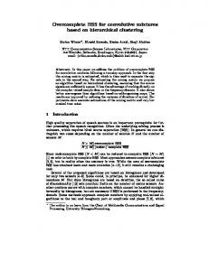
Figure 1: A synthetic MIMO mixing system. Here, two components were convolutively mixed at three sensors. The ’poles’ of the mixture (as defined in section 2.1) are all situated within the unit circle, hence an exact and stable inverse exists in the sense of (11).
9
Correlation coefficient
A
B
1
1
0.9
0.9
0.8
0.8
0.7
0.7 Rectangular Augmented Diminished
0.6 0.5 1
0.6 0.5
10 100 1000 SNR
1
10 100 1000 SNR
Figure 2: Comparison of separation of the system in Fig. 1 using three cICA approaches (Rectangular, Augmented, Diminished). A: Estimates of true component activity: correlations with the best-estimated component. B: Similar correlations for the less well estimated component. 3. (Diminished) Perform the decomposition with D equal to K, i.e. on a K-dimensional subspace projection of the data. We compared the performance of these three approaches experimentally as a function of signal-to-noise ratio (SNR). First, we created a synthetic mixture, two i.i.d signals s1 (t) and s2 (t) (with 1 ≤ t ≤ N and N = 30000) generated from a laplacian distribution, sk (t) ∼ p(x) = 12 exp(−|x|) with variance Var{sk (t)} = 2. These signals were mixed using the filters of length L = 30 shown in Figure 1 producing an overdetermined 3-D mixture (D = 3, K = 2). A 3-D i.i.d. P Gaussian noise signal nt was added to the mixture xt = σnt + Lτ=0 Aτ st−τ with a controlled variance σ 2 . Next, we investigated how well the three analysis approaches estimated the two components by measuring the correlations between each true component innovation, sk (t), and the best-correlated estimated component innovation, sˆk0 (t).
10
Approach 1 (Rectangular). Here, all three data channels were decomposed and the two true components estimated. Figure 2 shows how well the components were estimated at different SNR levels. The quality of the estimation dropped dramatically as SNR decreased. Even though our derivation (Section 2) is valid for the overdetermined case (D > K), the validity of the zero-noise assumption proves vital in this case. The explanation for this can be seen in the definitions of the likelihood (10) and unmixing filter (11). In (10), any rotation on the columns of A0 will not influence the determinant term of the likelihood. From (11) we note that the estimated component vectors D ˆst are found by linear mapping through A# 7→ IRK . Hence, the prior 0 : IR
term in (10) alone will be responsible for determining a rotation of A0 that hides as much variance as possible in the nullspace (IRD−K ) of A# 0 in (11). In an unconstrained optimization scheme, this side-effect will be untamed and consequently will hide variance in the nullspace of A# 0 and achieve an artificially high likelihood while relaxing the effort to make the components independent. Approach 2 (Augmented). One solution to the problem with the Rectangular approach above could be to parameterize the nullspace of A# 0 , or equivalently the orthogonal complement space of A0 . This can be seen as a special case of the algorithm in which A0 is D-by-D and Aτ is D-by-K. With the D −K additional columns of A0 denoted by B, the model can be written xt = Bvt +
L X
Aτ st−τ
(18)
τ =0
where vt and B constitute a low-rank approximation to the noise. Hence, we declare a Gaussian prior p.d.f. on vt . Note that (18) is a special case of the convolutive model (1). In this case, we attempt to estimate the third (noise) component in addition to the two convolutive components. Figure 2 shows how well the components are estimated using this approach for different SNR levels. For the best estimated component (Fig. 2-A), the 11
Augmented approach gave better estimates than the Rectangular or Diminished approaches. This was also the case for the second component (Fig. 2-B) at low SNR, but not at high SNR since in this case the ’true’ B was near zero and became improbable under the likelihood model. Approach 3 (Diminished). Finally, we investigated the possibility of extracting the two components from a two-dimensional projection of the data. For example, in the EEG experiment later in this paper, we will propose to project the data onto a subspace defined by K instantaneous ICA components. In other situations, PCA might be a more principled way to dimensionality reduction. However, for the current synthetic experiment we pick a more random projection, simply by excluding the third ’sensor’ from the decomposition. Figure 2 shows that even in the presence of considerable noise, the separation achieved was not as good as in the Augmented approach. However, the Diminished approach used the lowest number of parameters and hence had the lowest computational complexity. Furthermore, it lacked the peculiarities of the Augmented approach at high SNR. Finally we note that once the Diminished model has been learned, an estimate of the Rectangular model can be obtained by solving < xt sTt−λ > =
X
Aτ < st−τ sTt−λ >
(19)
τ
for Aτ by regular matrix inversion using the estimated components and < · >= PN 1 1=1 . N Summary of the three approaches. In the presence of considerable noise, the best separation was obtained by augmenting the model and extracting, from the D-dimensional mixture, K components as well as a (rank D−K) approximation of the noise. However, the Diminished approach had the advantage of lower computational complexity, while the separation it achieved was close to that of the Augmented approach. At very high SNR, the Diminished approach was 12
even slightly better than the Augmented approach. The Rectangular approach, meanwhile, had difficulties and should not be considered for use in practice as the presence of some channel noise may be assumed.
4
Detecting a convolutive mixture
Model selection is a fundamental issue of interest, in particular, detecting the order of L can tell us whether the convolutive mixing model is a better model than the simpler instantaneous mixing model of standard ICA methods. In the framework of Bayesian model selection, models that are immoderately complex are penalized by the Occam factor, and will therefore only be chosen if there is a relevant need for their complexity. However, this compelling feature can be disrupted if fundamental assumptions are violated. One such assumption was involved in our derivation of the likelihood, in which we assumed that the components are iid, i.e. not auto-correlated. The problem with this assumption is that the likelihood will favor models based not only on achieved independence but on component whiteness as well. A model selection scheme for L which does not take the component auto-correlations into account will therefore be biased upwards because models with a larger value for L can absorb more component auto-correlation than models with lower L values. To address this problem, we introduce a model for each of the sources sk (t) =
M X
hk (λ)zk (t − λ)
(20)
λ=0
where zk (t) represents an i.i.d. signal—a whitened version of the component signal. Introducing the K component filters of order M allows us to reduce the value of L, i.e. lowering the number of parameters in the model while achieving uniformly better learning for limited data [Dyrholm et al., 2006]. We note that some authors of FIR unmixing methods have also used component models, e.g. [Pearlmutter and Parra, 1997; Parra et al., 1997; Attias and 13
Schreiner, 1998].
4.1
Learning component auto-correlation
The negative log likelihood for the model combining (1) and (20) is given by L = N log | det A0 | + N
X
log |hk (0)| −
N X
log p(ˆzt )
(21)
t=1
k
where zˆt is a vector of whitened component signal estimates at time t using an operator that represents the inverse of (20), and we assume A0 to be square as in the Diminished and Augmented approaches above. We can without loss of generality set hk (0) = 1, then L = N log | det A0 | −
N X
log p(ˆzt )
(22)
t=1
For notational convenience we introduce the following matrix notation instead of (20), bundling all components in one matrix equation st =
M X
Hλ zt−λ
(23)
λ=0
where the Hλ ’s are diagonal matrices defined by (Hλ )ii = hi (λ). To derive an algorithm for learning the component auto-correlations in addition to the mixing model we modify the equations found in Section 2.2; inserting a third, Component model step (see below) between the two steps found there, i.e. substituting zˆt for ˆst in step two. Component model step The inverse component coloring operator is given by zˆt = ˆ st −
M X
Hλ zˆt−λ
(24)
λ=1
and the partial derivatives, which we shall use in step two, are given by M
X ∂(ˆ zt )k ∂(ˆ st )k ∂(ˆ zt−λ )k = − Hλ −1 −1 ∂(A0 )ij ∂(A0 )ij λ=1 ∂(A−1 0 )ij 14
(25)
M
X ∂(ˆ zt−λ )k ∂(ˆ zt )k ∂(ˆ st )k = − Hλ ∂(Aτ )ij ∂(Aτ )ij λ=1 ∂(Aτ )ij ! ÃM X ∂(ˆzt )k ∂ˆzt−λ0 = −δ(k − i)(ˆzt−λ )i − Hλ0 ∂(Hλ )ii ∂(Hλ )ii λ0 =1
(26)
(27) k
Step two modified — Gradient of the cost-function The gradient of the cost-function with respect to A−1 0 with the component model invoked is given by N
X ∂ˆzt ∂L({Aτ }) T = −N (A ) − ψ Tt ij 0 −1 ∂(A0 )ij ∂(A−1 0 )ij t=1
(28)
and the gradient with respect to the other mixing matrices is N
X ∂L({A}) ∂ˆzt =− ψ Tt ∂(Aτ )ij ∂(Aτ )ij t=1
4.2
(29)
Protocol for detecting L
We propose a simple protocol for determining the dimensions (L, M ) of the convolutional and component filters. First, expand the convolution without an autofilter (M = 0). This will model the total temporal dependency structure of the system Lmax . The optimal dimension is found by monitoring the Bayes Information Criterion (BIC) [Schwarz, 1978] log p(M|X) ≈ log p(X|θθ 0 , M)−
dim θ log N 2
(30)
where M represents a specific choice of model structure (L, M ), θ represents the parameters in the model, θ 0 are the maximum likelihood parameters, and N is the size of the data set (number of samples). Next, keep the temporal dependency constant, (L + M ) = Lmax , while expanding the length of the component auto-filters M , again monitoring the BIC to determine the optimal choice of L = Lmax − M .
15
Source 1
Source 2
1 0 -1 0
5 10 Filter lags
15 0
5 10 Filter lags
15
Figure 3: These filters are used to produce autocorrelated components (M = 15).
4.3
Example: Correctly rejecting cICA of an instantaneous mixture
We will now illustrate the importance of the component model and the validity of the protocol for detecting L when dealing with the following fundamental question: Do we learn anything by using convolutive ICA instead of instantaneous ICA? Or, put in another way, Should L be larger than zero? To produce an instantaneous mixture we now generate two random signals from a Laplace distribution, filter them through filters of order 15 shown in Figure 3, and mix the two filtered components using an arbitrary square mixing matrix. Figure 4A shows the result of using Bayesian model selection for this mixture without allowing for a filter (M = 0). This corresponds to model selection in a conventional convolutive model. Since the signals are non-white, L is detected and the model BIC simply increases as function of L up to the maximum, here stopped at L = 15. Next, (Fig. 4B) we fix L + M = 15. Models with a larger L have at least the same capability as models with lower L, though models with lower L are preferable because they have fewer parameters. By adding the component model, we get the correct answer in this case: These data contain no evidence of convolutive mixing.
16
Bayes Info. Criterion (/1000)
-30 -32 -34 -36 -38 -40 -42 -44 -46 -48
A
-31.6
B
-31.7
-31.8 0 5 10 15 20 25 # Lags (L)
0
5 10 15 # Lags (L)
Figure 4: A: The result of using Bayesian model selection without allowing for an autofilter (M = 0). Since the signals are non-white, the validity of L is unquestioned even at 15 lags (L = 15). B: We fix L + M = 15, and now get the correct answer, that model information is largest for L = 0, meaning there is no evidence of convolutive mixing.
5
Deconvolving an EEG ICA subspace
We will now show by example how cICA can be used to separate the delayed influences of statically defined ICA components on each other, thereby achieving a larger degree of independence in the convolutive component time courses. The procedure described here can be seen as a Diminished approach in which we extract K convolutive components from the D-dimensional data by deconvolving a K-dimensional subspace projection of the data. In [Dyrholm et al., 2004] we used a subspace from Principal Component Analysis (PCA), but as our experiment will show, using ICA for that projection has the benefit that the subspace can be chosen e.g. for physiological interest. As a first test of this approach, we applied convolutive decomposition to 20 minutes of a 71-channel human EEG recording (20 epochs of 1 minute duration), downsampled for numeric convenience to a 50-Hz sampling rate after
17
filtering between 1 and 25 Hz with phase-indifferent FIR filters. First, the recorded (channels-by-times) data matrix (X) was decomposed using extended Infomax ICA [Bell and Sejnowski, 1995; Makeig et al., 1996; Jung et al., 1998; Lee et al., 1999; Jung et al., 2001] into 71 maximally independent components whose (’activation’) time series were contained in (components-by-times) matrix SICA and whose (’scalp map’) projections to the sensors were specified in (channels-by-components) mixing matrix AICA , assuming instantaneous linear mixing X = AICA SICA . Five of the resulting independent components (ICs) were selected for further analysis on the basis of event-related coherence results that showed a transient partial collapse of component independence following the subject button presses [Makeig et al., 2004b] — more specifically, all five components displayed amplitude activity that was time-locked to the subject button-presses, which was evident from looking at ‘ERP images’ of stimulus-aligned epochs sorted by button-press response time [Makeig et al., 2002]. The scalp maps of the five components, i.e. the relevant five columns of AICA , are shown on the left margin of Figure 7. Next, cICA decomposition was applied to the five component activation time series (relevant five rows of SICA ), assuming the model sICA t
=
L X
Aτ scICA t−τ
(31)
τ =0
As a qualified guess of the order L, we applied the approach to estimating L outlined in Section 4.2 above to the EEG subspace data. First, we increased the order of the convolutive model L (keeping M = 0) while monitoring the BIC. To produce error bars, we used jackknife resampling [Efron and Tibshirani, 1993]; i.e. for each value of L, 20 runs with the algorithm were performed, one for each jackknifed epoch, thus the data in each run consisted of the 19 remaining epochs. Figure 5A shows the mean jackknifed BIC. Clearly, the BIC, without an autofilter included, was at least Lmax = 40, since some correlations in the data extended 18
Jackknife BIC (/104)
-36 -38 -40 -42 -44 -46 -48
A
-36.1 -36.2 -36.3 -36.4 -36.5 -36.6 -36.7 -36.8 -36.9 -37
M=0 0 10 20 30 40 # Lags (L)
B
M+L=40 0
5 10 15 20 # Lags (L)
Figure 5: Using the protocol for detecting the order of L for EEG. A: There are correlations over at least 40 lags in the data. This corresponds to 800ms. B: By introducing the component model it turns out that L should only be on the order of 10 corresponding to 200 ms. to at least 800 ms. Next, we swept the range of possible component model filters M , keeping L + M = 40. Figure 5B shows that L = 10, corresponding to a filter length of 200 ms, proved optimal. Figures 6 shows the 5 × 5 matrix of learned convolutive kernels. Before plotting, we arranged the order of the five output CCs so that the diagonal (CCi → ICi ) kernels, shown in one-third scale in Fig. 6, were dominant. Figure 7 shows the resulting percent of variance of the contributions from each of the CC innovations to each of the IC activations. As the large diagonal contributions in Figure 7 show, each convolutive CCj dominated one spatially static IC (ICj). However, there were clearly significant off-diagonal contributions as well, indicating that spatiotemporal relationships between the static ICA components was captured by the cICA model. To explore the robustness of this result further, we tested for the presence of delayed correlations, first between the static IC activations (sICA k0 (t)) and then between the learned CC innovations (scICA (t)). Figure 8 shows, for the most k predictable IC and CC, the percent of their time course variances that was 19
CC1 -> IC1
CC2 -> IC1
CC3 -> IC1
CC4 -> IC1
CC5 -> IC1
CC1 -> IC2
CC2 -> IC2
CC3 -> IC2
CC4 -> IC2
CC5 -> IC2
CC1 -> IC3
CC2 -> IC3
CC3 -> IC3
CC4 -> IC3
CC5 -> IC3
CC4 -> IC4
CC5 -> IC4
x/3
x/3
x/3 CC1 -> IC4
CC2 -> IC4
CC3 -> IC4
x/3 CC1 -> IC5
CC2 -> IC5
CC3 -> IC5
CC4 -> IC5
CC5 -> IC5
x/3
0
200 0
200 0 200 0 Filter lag (ms)
200 0
200
Figure 6: Kernels of the five derived convolutive ICA components (CCs), arranged (in columns) in order of their respectively contributions to the five static ICA components (ICs) (rows). Each CC made a dominant contribution to one IC; these were ordered so as to appear on the diagonal. Scaling of the diagonal kernels is one third that of the off-diagonal kernels.
20
CC1
CC2
CC3
CC4
CC5
49% 9%
26% 9%
26% 14%
14% 1%
1%
88% 8%
88% 1%
1% 1%
1% 1%
1%
IC3
32% 1%
66% 1%
66% 0%
0% 0%
0%
10%
10% 3%
4% 3%
82% 4%
82% 2%
2%
2% 1%
94% 1%
49% IC1
8%
IC2
32%
IC4
2% 1%
1%
IC5
2% 2%
94%
Figure 7: Percent variance of five static ICA components (ICs) accounted for by the five derived convolutive components (CCs). The IC scalp maps on the left are shown for interest. Contributions arranged on the diagonal are dominant. Squares represent the (rounded) percent variance of the IC activation time series accounted for by each CC. Significant off-diagonal elements indicate the presence of significant delayed spatiotemporal interactions between the static IC
Predictability (%)
activations.
10 8 6 4
ICA cICA
2 0 0
2 4 6 8 Prediction order (r)
10
Figure 8: Predictability of the most predictable ICA component activation (IC3) and cICA component innovation (CC5) from the most predictive other IC and CC component, respectively (IC1, CC3). 21
accounted for by linear prediction from the past history (of order r) of the largest contributing remaining ICs or CCs, respectively. As expected from the cICA results, as the prediction order (r) increased, the predictability of the static ICA component activation also increased. For the ICA component activation, 9% of the variance could be explained by linear prediction from the previous 10 time points (200 ms) of another ICA component. The static ICA component time courses were nearly ’independent’ only in the sense of zero-order prediction (r = 0), as expected from their derivation. Their lack of independence at other lags is compatible with the cICA results. For the CC innovation, however, the predictability in Figure 8 remained low as r increased, indicating that cICA in fact deconvolved delayed correlations present in the EEG subspace data. Figure 9 shows the power spectral densities for each of the IC activations (in bold traces) along with the two CCs (in thin traces) that, in accordance with Figure 7, contributed the most to the respective IC (c.f. Figure 7). Note that the broad alpha band spectral peak in IC1 (uppermost panel in Figure 9) around 10Hz has been split between CC1 and CC3. In the middle panel, note the distinct spectral contributions of CC1 and CC3 to the double alpha peak in the IC3 spectrum. As expected, the CCs made different spectral contributions to the IC time courses. For example, CC1 made different power spectral density contributions to IC1, IC3 and IC4.
6
Discussion
In general, the usefulness of any blind decomposition method applied to biological time series data is most likely relative to the fit between the assumptions of the algorithm and the underlying physiology and biophysics. Therefore it is important to consider the physiological basis of the delayed interactions between statically-defined independent component time courses we observed here, 22
IC1 -80
CC1 (49%)
-120
CC3 (26%)
IC2 Power spectral density (dB)
-80
CC3 (8%)
-120
CC2 (88%)
IC3 -80
CC1 (32%) CC3 (66%)
-120
IC4 -80 CC4 (82%) CC1 (10%)
-120
IC5 -80 CC5 (94%)
-120 0
5
10 15 Frequency (Hz)
20
25
Figure 9: Power spectrum of the most powerful CC contributions to the five ICs.
23
and the possible physiological significance of the derived convolutive component filters and time courses. Applied to these EEG data static ICA gave 15–20 components that were of physiological interest according to their spatial projections or activation time series, although we were not able to practically de-convolve more than five components here because of numeric complexity. Open questions, therefore, are to identify independent component subspaces of interest for cICA decomposition or to explore the efficiency of performing cICA on larger computer clusters. In future, convolutive ICA might also be applied usefully to other types of biomedical time series data that involve stereotyped source movements, thus presenting problems for static ICA decomposition. These might include electrocardiographic (ECG) and brain hemodynamic measures such as diffusion tensor imaging (DTI) [Anem¨ uller et al., 2004].
References Anem¨ uller, J., Duann, J.-R., Sejnowski, T. J., and Makeig, S. (2004). Unraveling spatio-temporal dynamics in fmri recordings using complex ica. In Puntonet, C. G. and Prieto, A., editors, Independent Component Analysis and Blind Signal Separation, pages 1103–1110, Granada, Spain. Anem¨ uller, J. and Kollmeier, B. (2003). Adaptive separation of acoustic sources for anechoic conditions: A constrained frequency domain approach. IEEE Transactions on Speech and Audio Processing, 39(1-2):79–95. Anem¨ uller, J., Sejnowski, T., and Makeig, S. (2003). Complex independent component analysis of frequency-domain eeg data. Neural Networks, 16:1313– 1325. Attias, H. and Schreiner, C. E. (1998). Blind source separation and deconvolution: the dynamic component analysis algorithm. Neural Computation, 10(6):1373–1424. 24
Baumann, W., Kohler, B.-U., K., D., and Orglmeister, R. (2001). Real time separation of convolutive mixtures. In Lee, T.-W., Jung, T.-P., Makeig, S., and Sejnowski, T. J., editors, 3’rd International Conference on Independent Component Analysis and Blind Signal Separation., pages 65–69, San Diego, CA, USA. Bell, A. and Sejnowski, T. J. (1995). An information maximisation approach to blind separation and blind deconvolution. Neural Computation, 7:1129–1159. ´ (1997). A Belouchrani, A., Meraim, K. A., Cardoso, J.-F., and Moulines, E. blind source separation technique based on second order statistics. IEEE Transacarions on Signal Processing, 42:434–444. Cardoso, J.-F. and Pham, D.-T. (2004). Optimization issues in noisy gaussian ica. In Puntonet, C. G. and Prieto, A., editors, Independent Component Analysis and Blind Signal Separation, pages 41–48, Granada, Spain. Choi, S. and Cichocki, A. (1997). Blind signal deconvolution by spatio- temporal decorrelation and demixing. In Principe, J., Gile, L., Morgan, N., and Wilson, E., editors, Neural Networks for Signal Processing, pages 426–435, Amelia Island, CA, USA. Choi, S., ichi Amari, S., Cichocki, A., and wen Liu, R. (1999). Natural gradient learning with a nonholonomic constraint for blind deconvolution of multiple channels. In Independent Component Analysis and Blind Signal Separation, pages 371–376, Aussois, France. Comon, P., Moreau, E., and Rota, L. (2001). Blind separation of convolutive mixtures: A constrast based joint diagonalization appraoch. In Lee, T.-W., Jung, T.-P., Makeig, S., and Sejnowski, T. J., editors, Independent Component Analysis and Blind Source Separation, pages 686–691, San Diego, CA, USA.
25
Deligne, S. and Gopinath, R. (2002). An em algorithm for convolutive independent component analysis. Neurocomputing, 49:187–211. Delorme, A. and Makeig, S. (2004). Eeglab: an open source toolbox for analysis of single-trial eeg dynamics. Journal of Neuroscience Methods, 134:9–21. Delorme, A., Makeig, S., and Sejnowski, T. J. (2002). From single-trial eeg to brain area dynamics. Neurocomputing, 44-46:1057–1064. Douglas, S. C., Cichocki, A., and Amari, S. (1999). Self-whitening algorithms for adaptive equalization and deconvolution. IEEE Transactions on Signal Processing, 47:1161–1165. Dyrholm, M. and Hansen, L. K. (2004). CICAAR: Convolutive ICA with an auto-regressive inverse model. In Puntonet, C. G. and Prieto, A., editors, Independent Component Analysis and Blind Signal Separation, pages 594–601, Granada, Spain. Dyrholm, M., Hansen, L. K., Wang, L., Arendt-Nielsen, L., and Chen, A. C. (2004). Convolutive ICA (c-ICA) captures complex spatio-temporal EEG activity. In 10th annual meeting of the organization for human brain mapping. Dyrholm, M., Makeig, S., and Hansen, L. K. (2006). Model structure selection in convolutive mixtures. In Rosca, J., Erdogmus, D., Pr´ıncipe, J. C., and Haykin, S., editors, Independent Component Analysis and Blind Signal Separation, pages 74–81, Charleston, USA. Efron, B. and Tibshirani, R. (1993). An Introduction to the Bootstrap. Chapman & Hall, New York. Hansen, P. C. (2002). Deconvolution and regularization with toeplitz matrices. Numerical Algorithms, 29:323–378.
26
Jung, T.-P., Humphries, C., Lee, T.-W., Makeig, S., McKeown, M. J., Iragui, V., and Sejnowski, T. J. (1998). Extended ICA removes artifacts from electroencephalographic recordings. In Jordan, M. I., Kearns, M. J., and Solla, S. A., editors, Advances in Neural Information Processing Systems. Jung, T.-P., Makeig, S., Humphries, C., Lee, T.-W., McKeown, M. J., Iragui, V., and Sejnowski, T. J. (2000). Psychophysiology, 37:163–78. Jung, T.-P., Makeig, S., McKeown, M. J., Bell, A., Lee, T.-W., and Sejnowski, T. J. (2001). Imaging brain dynamics using independent component analysis. Proceedings of the IEEE, 89(7):1107–22. Lee, T.-W., Bell, A. J., and Lambert, R. H. (1997a). Blind separation of delayed and convolved sources. In Mozer, M. C., Jordan, M. I., and Petsche, T., editors, Advances in Neural Information Processing Systems, pages 758–764. Lee, T.-W., Bell, A. J., and Orglmeister, R. (1997b). Blind source separation of real world signals. In International Conference Neural Networks, pages 2129–2135, Houston, TX, USA. Lee, T.-W., Girolami, M., and Sejnowski, T. J. (1999). Independent component analysis using an extended infomax algorithm for mixed sub-gaussian and super-gaussian sources. Neural Computation, 11(2):417–441. Makeig, S., Bell, A. J., Jung, T.-P., and Sejnowski, T. J. (1996). Independent component analysis of electroencephalographic data. Advances in Neural Information Processing Systems, 8:145–151. Makeig, S., Debener, S., Onton, J., and Delorme, A. (2004a). Mining eventrelated brain dynamics. Trends in Cognitive Science, 8(5):204–210. Makeig, S., Delorme, A., Westerfield, M., Townsend, J., Courchense, E., and Sejnowski, T. (2004b). Electroencephalographic brain dynamics following visual targets requiring manual responses. PLoS Biology. 27
Makeig, S., Enghoff, S., Jung, T.-P., and Sejnowski, T. J. (2000). A natural basis for efficient brain-actuated control. IEEE Trans. Rehab. Eng., 8:208–211. Makeig, S., Westerfield, M., Jung, T.-P., Enghoff, S., Townsend, J., Courchesne, E., and Sejnowski, T. J. (2002). Dynamic brain sources of visual evoked responses. Science, 295(5555):690–694. Mitianoudis, N. and Davies, M. (2003). Audio source separation of convolutive mixtures. IEEE Transactions on Speech and Audio Processing, 11(5):489–497. ´ Cardoso, J.-F., and Gassiat, E. (1997). Maximum likelihood for Moulines, E., blind separation and deconvolution of noisy signals using mixture models. In International Conference on Acoustics, Speech, and Signal Processing, pages 3617–3620, Munich, Germany. Neumaier, A. and Schneider, T. (2001). Estimation of parameters and eigenmodes of multivariate autoregressive models. ACM Transactions on Mathematical Software (TOMS), 27(1):27–57. Nielsen, H. B. (2000). Ucminf - an algorithm for unconstrained, nonlinear optimization. Technical Report IMM-REP-2000-19, Department of Mathematical Modelling, Technical University of Denmark. Onton, J., Delorme, A., and Makeig, S. (2005). Frontal midline eeg dynamics during working memory. NeuroImage, 27:342–356. Parra, L. and Spence, C. (2000). Convolutive blind source separation of nonstationary sources. IEEE Transactions on Speech and Audio Processing, 8:320– 327. Parra, L., Spence, C., and Vries, B. (1997). Convolutive source separation and signal modeling with ml. In International Symposium on Intelligent Systems, Reggio Calbria, Italy. 28
Parra, L., Spence, C., and Vries, B. D. (1998). Convolutive blind source separation based on multiple decorrelation. In Neural Networks for Signal Processing, pages 23–32, Cambridge, UK. Pearlmutter, B. A. and Parra, L. C. (1997). Maximum likelihood blind source separation: A context-sensitive generalization of ICA. In Mozer, M. C., Jordan, M. I., and Petsche, T., editors, Advances in Neural Information Processing Systems, pages 613–619. Rahbar, K. and Reilly, J. (2001). Blind source separation of convolved sources by joint approximate diagonalization of cross-spectral density matrices. In International Conference on Acoustics, Speech, and Signal Processing, pages 2745–2748, Salk Lake City, Utah, USA. Rahbar, K., Reilly, J. P., and Manton, J. H. (2002). A frequency domain approach to blind identification of mimo fir systems driven by quasi-stationary signals. In International Conference on Acoustics, Speech, and Signal Processing, pages 1717–1720, Orlando, Florida, USA. Schwarz, G. (1978). Estimating the dimension of a model. Annals of Statistics, 6:461–464. Sun, X. and Douglas, S. (2001). A natural gradient convolutive blind source separation algorithms for speech mixtures. In Lee, T.-W., Jung, T.-P., Makeig, S., and Sejnowski, T. J., editors, Independent Component Analysis and Blind Source Separation, pages 59–64, San Diego, CA, USA. Torkkola, K. (1996). Blind separation of convolved sources based on information maximization. In Neural Networks for Signal Processing, pages 423–432, Kyoto, Japan.
29