Modeling Arctic Ocean heat transport and warming episodes in the

Chinese Journal of Polar Science, Vol. 19,No. 2,159 -167, December 2008

Modeling Arctic Ocean heat transport and warming episodes in the 20th century caused by the intruding Atlantic Water Wang Jia 1 , Jin Meibing 2 , Jun Takahashi 3 , Tatsuo Suzuki3 Mizobata

4

,

Moto

Ikeda5 ,

Fancois 1.

Saucier6

and Markus

,

Igor V Polyakov l

,

Kohei

Meier7

1 NOAA Great Lakes Environmental Research Laboratory, 4840 S State Road, Ann Arbor, Michigan 48108, USA 2 International Arctic Research Center, University of Alaska Fairbanks, 930 Koyukuk Dr. , Fairbanks, AK 99775, USA 3 Frontier Research Center for Global Change, 3173-25 Showamachi, Kanazawa-ku, Yokohama City, Kanagawa 236'{)()()1 , Japan

4 Department of Ocean Science, Tokyo University of Marine Science and Technology, Tokyo, Japan 5 Graduate School of Earth and Environmental Science, Hokkaido University, Sapporo, Hokkaido, Japan 6 Institute of Ocean Science, University of Quebec at Rimouski, 310 Ursulines Street, Rimouski, G5L 3AJ Canada 7 Rossby Centre, Swedish Meteorological and Hydrological Institute, Sweden

Received September 20, 2008 Abstract

This study investigates the Arctic Ocean warming episodes in the 20th century using both a high-resolution coupled global climate model and historical observations. The model, with.no flux adjustment, reproduces well the Atlantic Water core temperature (AWCT) in the Arctic Ocean and shows that four largest decadalscale warming episodes occurred in the 1930s, 70s, 80s, and 90s, in agreement with the hydrographic observational data. The difference is that there was no pre-warming prior to the 1930s episode, while there were two pre-warming episodes in the 1970s and 80s prior to the 1990s, leading the 1990s into the largest and prolonged warming in the 20th century. Over the last century, the simulated heat transport via Fram Strait and the Barents Sea was estimated to be, on average, 31. 32 TW and 14. 82 TW, respectively, while the Bering Strait also provides 15.94 TW heat into the western Arctic Ocean. Heat transport into the Arctic Ocean by the Atlantic Water via Fram Strait and the Barents Sea correlates significantly with AWCT (C = 0.75) at 0lag. The modeled North Atlantic Oscillation (NAO) index has a significant correlation with the heat transport (C = 0.37). The observed AWCT has a significant correlation with both the modeled AWCT ( C = 0.49) and the heat transport (C = 0.41) . However, the modeled NAO index does not significantly correlate with either the observed AWeT (C = O. 03) or modeled AWCT (C = O. 16) at a zero-lag, indicating that the Arctic climate system is far more complex than expected. Key words Arctic Ocean, heat transport, warming episodes, modeling.

160

1

Wang Jia et al.

Introduction

The Arctic atmosphere experienced significant wanning over the 20th century, which can be measured by the first leading mode of Arctic sea-level pressure ( SLP) and surface air temperature ( SAT) [ 1-3]. These indices show that there were several wanning episodes in the 1930s, 70s, 80s, and 1990s, with the 1990s being the largest and longest and the 1930s being the second (see Fig. 5 of Thompson and Wallace 1998 [1] and Fig. 8 of Wang et at. 2005[3]). Polyakov et at. (2002) [4] found that the 1930s and 1990s warmings were comparable in magnitude in the Arctic maritime SAT and may be attributed to natural multidecadal variability [2] . Bengtsson et at. (2004) [5] investigated a possible mechanism of the 1930-40 wanning. These warming episodes are generally attributed to the Arctic Oscillation (AO) [1,3] or the North Atlantic Oscillation (NAO). The Atlantic Water is considered the heat engine that persistently supplies heat to the Arctic Ocean via Fram Strait and the Barents Sea to maintain the Arctic Ocean heat balance [6-11 ]. Therefore, the Atlantic Water/Layer in the Arctic Ocean is a key parameter to measure the Arctic wanning episodes. Polyakov et at. (2004) [12] revealed the long-term variability of the Atlantic Water core temperature (AWCT) using historical measurements over the last 100 years. They found similar wanning episodes in the 1930s and 1990s with comparable magnitude in the Arctic intermediate Atlantic Water. Wang et at. (2005) [3] proposed a decadal time scale Arctic climate feedback loop, in which the Atlantic Water intrusion into the Arctic Ocean is a key component in the Arctic climate system. There have been many efforts to investigate the Arctic Atlantic Water using regional ocean-ice models, primarily for the short-term variability [ 13]. Regional ocean-ice models have difficulty in reproducing the natural variability due to the following limitations: 1) the southern boundary cuts off the interaction between the Arctic and the subpolar oceans such as the Atlantic Ocean and Bering Sea [3] , 2) flux adjustment and!or restoring of temperature and salinity to climatological values in the interface, the ocean interior and boundaries have to be prescribed to avoid a model s drift away from climatology, which has been shown to be a damping factor for long-term variability [14] , and 3) long-term integration of regional models is always problematic because the energy (heat) and mass (freshwater) budgets are not closed. It is also a great challenge even for global climate models to simulate the Arctic Water of the Atlantic origin due to model resolution, numerical accuracy, and a lack of understanding of physical processes. Most global models use the so-called flux adjustment or restoring in order to perform a long-term integration. Nevertheless, there have been no reports that the Atlantic Water was successfully reproduced. The objective of this study is to evaluate long-term natural variability of the intermediate Atlantic Water of the Arctic Ocean intrinsic to the coupled atmosphere-ocean-sea ice climate system using a high-resolution, coupled global climate model with no restoring or flux adjustment constraint.

2

CCSRlNIES/FRCGC climate model

The CCSRlNIES/FRCGC coupled atmosphere-ice-ocean climate model is the Model for Interdisciplinary Research on Climate (MIROC) version 3. 2, which was developed by

Modeling Arctic Ocean heat transport and warming episodes in the'20th century ...

161

the Center for Climate System Research (CCSR), University of Tokyo, National Institute for Environmental Studies (NIES), and Frontier Research Center for Global Change ( FRCGC) [15 J. This model was configured in the Earth Simulator (ES) and has the following features: 1) the atmosphere model has Tl06 ( - 1. 1 0) spectral resolution with 56 vertical levels, 2) the ocean model resolution is 1I4°x1l6° with 48 levels with the north pole rotated to Greenland, 3) the sea ice model uses a single level ice model with elastic-plasticviscous rheology[16 J . The model was parallelized with a message-passing interface (MPI) on 80 processors for the atmosphere model and 608 processors for the ocean-ice model. The initial ocean temperature and salinity use the climatology of Levitus and Boyer (1994) [17J. The coupled model was spun up for 109 years under the climate forcing of 1900, including atmospheric (greenhouse gases, solar radiation, aerosol, volcano eruptions, etc. ). Then the model was integrated from 1900 to 2000. Note that throughout the spinup and simulation, neither restoring method nor flux adjustment was used[ 18].

3

Atlantic Water variability and warming episodes in the 20th century 2.5

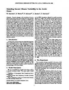
Monthly model temp. ........ 25 month running mean model temp. 2.0 - - Data

1910 1920 1930 1940 1950 1960 1970 1980 1990 Fig. 1

Time series of the normalized anomalies of the AWCT simulated by the model (black, with the 25-month running mean in yellow) and by observation (in red) [12]. The correlation is O. 49, above the 95% significance level of 0.35 determined by the Monte Carlo simulation[26] ).

Figure 1 shows the simulated 100-year time series of the normalized AWCT and observed Awct , using the same regionally-normalized method as Polyakov et at. (2004) [12] , who defined the AWCT anomaly as the maximum temperature anomaly in the water column below 50 m, divided by its standard deviation. Over the 20th century, the modeled AWCT compares very well with the observations, with a temporal correlation of 0.49 (see Table 1). For example, the model reproduces the 1930s warming with a smaller amplitude than the observation. The model also reproduces three consecutive warming episodes in the late 1970s, 1980s, and 1990s, with the 1990s warming being the largest and longest [ 10 J , which may extend to 2004 [8]. However, the model shows a warming event in the 1970 s, opposite to a cooling event in the observation. This could be due to the fact that the data used to calculate the AWCT were taken in the deep ocean, while the warming epi-

162

Wang lia et

at.

sode in the 1970s in the model occurred in the shallow seas, as shown and discussed shortly. The model captures very well the warming episodes in the 1980s and 90s, even with a larger magnitude. The correlation between time series of the AWCT derived from the simulations and the observation is 0.49 with the 95% significance level of 0.35 (see Table 1). The relatively low correlation may be due to the out of phase in the 1970s. It is clear that both the coupled model and the observations capture the multi-decadal (5Q-80 years) variability over the last century. As shown in Table 1, the modeled AWCT has very high correlation with total heat transport (0.75). The correlation with the Fram Strait heat transport alone is 0.68, implying the Barents Sea heat transport is also an important contributor. As expected, the modeled NAO index has a significant correlation (0.37) with heat transport from Fram Strait and the Barents Sea. Table 1.

Correlation and significance level using Monte Carlo simulation. Obs. -T and Mod. -T denote the observed and modeled AWCT, respectively j Mod. -NAOI is the modeled NAO index j HT denotes heat transport; and FS and BS denote the Fram Strait and the Barents Sea, respectively. The correlations were computed for the period of 1925 to 1999. due to missing data before 1925. The correlations (before slash) over the 95 % significance level (after slash) are bold. The first ~olumn time series were randomized to determine the significance levels by a Monte Carlo approach Randomized Obs. -T Mod. -T Mod. -NAOI HT/FS + BS HT/FS Obs. -T Mod. -T

Mod. -NAOI HT/FS +BS

0.49/0.35

0.03/0.25 O. 16/0.25

0.41/0.31

0.43/0.31

0.75/0.41

0.6810.37

0.37/0.27

0.35/0.25 0.91/0.33

However, the correlation between the modeled AWCT and the NAO index is only 0.16, below the 95% significance level of 0.25. This indicates that the AWCT variability in the Arctic Ocean has a weak association with the NAO, although NAO-related wind (i. e, , atmospheric circulation) in the northern North Atlantic Ocean is considered the major driver of the warm, saline Atlantic Water intruding into the Arctic Ocean at the intraseasonal and interannual time scales [ 10,11 ] . For example, in the late 1990s, the NA0 index dropped to around zero and even negative values, while the AWCT still experienced the prolonged warming based on both the model results and observations (see Fig. 2). In other words, the NAO has a phase difference with the heat transport and AWCT, which could be explained by the decadal feedback loop in the Arctic climate system [3 ]. This association is more complex than can be shown by simple O-lag correlation. Figure 2 shows that the NAO is a much faster process than the oceanic heat flux and AWCT variability. This is a natural , fundamental difference between the atmosphere. and the ocean. The Arctic climate is a fully coupled atmosphere-sea ice-ocean system and should be described by a feedback loop as proposed by Wang et at. (2005) [3]. In addition, the Arctic Ocean has its own time scale depending on its basin size and baroclinic (internal) Kalvin wave progression[ 19] , which may redistribute heat content inside the Arctic Ocean. It should be noted that the 1930s warming was a natural variability at time scales of 50-80 years [ 12] , which was captured by the climate model in terms of magnitude and phase. The coincidence of phasing is likely due to the prescribed solar output, aerosol, volcano eruptions, etc. in the last century [20] . To examine the spatial pattern of the warming episodes, decadal-averaged heat content

\1odeliny; Arclic Ocean tueat lransport and warming episodes in the 20th century ...

163

anomalies in the pan-Arctic were constructed for all ten decades. In the Arctic Ocean there were warming episodes in the 1930s, 1970s, 1980s, and 1990s (Fig. 3 ). During the 1920s, there was a cooling event, while just after the 1930s warming, a pulse of anomalous cold water intruded into the eastern Arctic Ocean via ham Strait and the Barents Sea, while the western Arctic was still experienced the prolonged warming since the 1930s. 3-

2

'"

V

-3 -4

-HT ofFS+BA2+BA3

-AW max lemp -NAO index from ES model

c-

I 900 191019201930 19401950 196019701980 19902000

Fig. 2

Time series of normalized anomalies of modeled AWCT ( pink) , heat transport from both Fram Strait and the Barents Sea (blue) • and the modeled winter (DJF) NAO index (black). The correlation between the NAO index and AWCT is O. 16 (not significant) and with the heat transport is O. 37 (significanl).

150

O.IOE+II g.60E+IO AOE+IO 0.20E+10 O.15E+10 O.IOE+IO p.50E+09 ).00 -O.50E+09 -0.1 OE+ 10 -0.15E+10 -O.20E+ 10 -OAOE+ 10 -0.60E+10 -O.IOE+ll

120 90 60 30

210

210

X.IO +11 .60E+IO B.40E+10 ).20E+10 0.15E+IO O.IOE+IO 0.50E+09 0.00 -0.50E+09 -O.IOE+IO -0.15E+IO

120

-O.20~+1O

-OAO 10 -0.60E+10 -O.IOE+II

o Fig. 3

42

X4

126

168

210

0

42

Decadal averaged heat content anomalies in March (in Joules m) aged velocity anomalies.

Therefore, the 1930s warming episode was a relatively short event, compared to the 19905. In the late 19705, a pulse of warming anomaly was advected into the eastern Arctic Ocean

164

Wang Jia et ai.

mainly along the coast from the Barents-Kara-Laptev-East Siberian seas. This may be the reason that the measurements missed this event since the data taken were from the deep basin (see Fig. 1 of Polyakov et at. 2004 [12J ). Extending into the 199Os, a decade-long warming episode occurred throughout the Arctic Ocean and was successfully detected and simulated [10 J. This warming evidently led to the retreat or collapse of the Arctic halocline layer[21 J , the anomalously-cyclonic regime of the ocean circulation [22J , and the shrinkage of Arctic sea ice[2,3J. The warming episode in the 1990s was attributed in part to the preconditioning of warming episodes in the 1970s and 80s. Since both Fram Strait and the Barents Sea are the major pathways for the advective heat transport from the Fram Strait of the Atlantic Water and the Bering Strait is the pathway for the Pacific Water, we calculated the modeled time series of year-to-year variability of heat transport (Fig. 4). The loo-year averaged net heat transports (relative to OCC water temperature) into the Arctic Ocean via Fram Strait, the Barents Sea, and Bering Strait are 31.32, 14.82 (BA2 + BA3) , and 15.93 TW (1 TW =10 12 Watts) , respectively (see Table 2 ). The Atlantic Water heat transport accounts for about three fourth (3/4) of the total transport, while the Pacific Water contributes about one fourth (1/4 ). We also calculated the heat transport from the Atlantic into the Barents Sea (see BAI section) , which is 129. 11 TW. In other words, nearly 89% of the heat is released to the atmosphere in the Barents Sea on the way to the Arctic Ocean, indicating that the Barents Sea is the most active region in terms of air-sea interactions. Heat transport from Bering Strait (15.93 TW) ,is comparable to that from the Barents Sea (14. 82 TW). Thus, the Bering Sea contribution to the Arctic heat balance and sea ice retreat is important. 120

100

-+-BS -FS -BA2+BA3 - - BS+FS+FA2+BA3 • FS by Schauer (2004)

-20 L-_L.-_"'---_"'-_..L..-_-'-_-'-_-'-_-'-_---'-_....J 1 900 1 910 1 920 1 930 1 940 1 950 1 960 1 970 I 980 1 990 2 000 Fig.4

The annual time series of model-simulated heat transports (in units of 10 12 Watts, or TW) from Fram Strait (gray) , the Barents Sea (black), Bering Strait (red), and the total (pink). The observations in Fram Strait with tbe standard deviations by Schauer et ai. (2004) (6] were in blue.

The observed heat transport during 1997/98 was lower than the model results, even in terms of standard deviations[6J , while the observed heat flux during 1998/99 was compara-

Modeling Arctic Ocean heat transport and wanning episodes in the 20th century ...

165

ble to the model results ( Fig. 5). Note that heat flux derived from the measurements also contains errors due to horizontal and vertical resolutions of the measurement arrays and the methods used to calculate the geostropic velocity based on ship-based measured temperature and salinity[23]. Walczowski et at. estimate that the heat flux into the Arctic Ocean from the West Spitsbergen Current was as high as 70 TW with a transport of 11. 6 Sv (1 Sverdrup =106 m3s - I) in the summer of 2003. -;

\)1,\

00

o

··0

~

Fig. 5

Arctic Ocean transects for calculating heat flux transport (see Table 2) : FS-Fram Strait, BA-Barents Sea, KS-Kara Sea, BS-Bering Strait, and BB-Baffin Bay.

Table 2.

4

Simulated heat flux transport (TW) and standard deviation in selective transects (see Fig. 5 for locations) FS BS BB2 BA3 BAI BA2 KS BBI

Mean

31.32

129. II

18.58

-2.77

7.67

15.94

0.03

1. 52

STD

17.85

32.03

15.12

4.70

7.81

20.47

1. 17

2.83

Conclusions

Several warming episodes of the Arctic Ocean at a decadal time scale in the 20th century have been reproduced by the CCSRlNIES/FRCGC high-resolution climate model with no flux adjustment. The finding was validated by AWCT historical measurement. The 1930s warming was shown to be short-lived compared to the 1990s warming. The 1990s warming brought the ocean temperatures to their highest levels of the century because of the preconditioning of the prior two consecutive warming episodes in the later 1970s and the 1980s. The 1970s warming mainly occurred along the coastal seas in the Barents-Kara-Laptev-East Siberian seas. The unprecedented high temperatures in the 1990s w~re associated with retreat or collapse of the Arctic Ocean halocline, an anomalously-cyclonic circulation regime, and sea ice shrinking and thinning. The results imply the Arctic environment is changing and may be heading to a new state[24,25]. This study sheds new light on the warming episodes associated with Atlantic heat flux transport into the Arctic Ocean, which has been re-

166

Wang Jia et al.

lated to the NAO-related wind forcing. Based on the computation of heat flux transport, Fram Strait is the major pathway (31. 32 TW) , while the Barents Sea (14. 82 TW) is the second as a pathway for the Atlantic Water intrusion. The Pacific Water also contributes 15.94 TW to the western Arctic. This high-resolution model run in the Earth Simulator, for the first time, reproduces these episodes that are validated by observations. This represents a major advance in simulating a coupled system with no constraint by the so-called restoring conditions or flux adjustment. Since the NAO index has a weak correlation with both the modeled and observed AWCT (Table 1) at a zero-lag, we further calculated the lag correlation. The lag correlations do not improve the results. The coupled atmosphere-sea ice-ocean coupled system is therefore complex. The climate feedback loop proposed by Wang et at. ( 2005) [3] provides a framework for future investigation of the very complex nature of the Arctic climate system. Acknowledgements We were supported by the Frontier Research Center for Global Change and International Arctic Research Center, through JAMSTEC, Japan. The climate model was rim on the Earth Simulator of JAMSTEC, Yokohama, Japan. Constructive discussions with Drs. T. Matsuno, T. Tokioka and N. Suginohara of FRCGC/JAMSTEC, and Dr. A. Sumi of CCSRlUT are very much appreciated. JW also thanks NOAA Office of Arctic Research for partial support. This is GLERL Contribution No. 1496. References [ I] [ 2] [ 3]

Thompson DWJ, Wallace JM ( 1998) : The Arctic Oscillation signature in the wintertime geopotential height and temperature fields. Geophys. Res. Lett. , 25: 1297 -1300. Wang J, Ikeda M( 2(00) : Arctic Oscillation and Arctic Sea-Ice Oscillation. Geophys. Res. Lett. , 27: 1287 -1290. Wang J, Ikeda M, Zhang S, Gerdes R ( 2005) : Linking the northern hemisphere sea ice reduction trend and the quasi-decadal Arctic sea ice oscillation. Climate Dyn. , 24: 115 - 130, DOl: 10. 10071s00382004~54-5.

[ 4] [ 5] [ 6]

[ 7] [ 8] [ 9] [ 10]

[11]

Polyakov IV et al. (2002) : Observationally based assessment of polar amplification of global Warming. Geophys. Res. Lett. , 29: 1878, doi: 1029/2001 GWlllll. Bengtsson L, Semenov VA, Johannessen OM (2004 ) : The early twentieth-eentury warming in the Arctic-A possible mechanism. J. Climate, 4045 -4057. Schauer U, Fahrbach E, Osterhus S, Roterhus G( 2004 ) : Arctic warming through the Fram Strait: Oceanic heat transport from 3 years of measurements. 1. Geophys. Res., 109: C06026 , doi: 10. 1029/ 2oo3/JCooI823. Schlichtholz P, Goszczko 1(2005) : Was the Atlantic water temperature in the West Spitsbergen Current predictable in the 1990s? Geophys. Res. Lett. , 32, L, doi: 10. 1029/2004GW21724. Polyakov IV et al. (2005): One more step toward a warmer Arctic. Geophys. Res. Lett., 32: L17605, doi: 10. 102912005GW2374O. Zhang J. Rothrock D, Steele M(2000) : Recent changes in Arctic sea ice: the interplay between ice dynamics and thennodynamics. J. Climate, 13:3099 - 3114. Karcher MJ, Gerdes R, Kauker F, Koberle C( 2003 ) : Arctic warming: Evolution and spreading of the 1990s warm event in the Nordic seas and the Arctic Ocean. J. Geophys. Res., 108: 3034, doi: 10. 1029/2001 JCoo1265. Wang J, WU B, Tang C, Walsh JE, Ikeda M( 2004) : Seesaw structure of subsurface temperature anomalies between the Barents Sea and the Labrador Sea. Geophys. Res. Lett., 31: Ll9301, doi: 10.·

Modeling Arctic Ocean heat transport and wanning episodes in the 20th century ...

[ 12 J [ 13 J

[ 14 J [15J

[16 J [17 J [ 18 J

[ 19 J [20 J

[21 J [22J [23 J [24 J

[25 J

167

1029/2004Gl.019981. Polyakov IV et at. (2004): Variability of the intermediate Atlantic Water of the Arctic Ocean over the last 100 years. J. Climate, 17(23) :4485 -4497. Maslowski W, Marble D, Walcwwski W, Schauer U, Clement JL, Semtner AJ (2004 ) : On climatological mass, heat, and salt transports through the Barents Sea and Fram Strait from a pan-Arctic coupled ice-ocean model simulation. J. Geophys. Res. , 109: C03032, doi: 10. 1029/200IJCOOI039. Simmons H, Polyakov IV (2004 ) : Restoring and flux adjustment in simulating variability of an idealized ocean. Geophys. Res. Lett. , 31: L16301, doi: 10. I029/2004GL0201 97 . K-I Model Developers (2004): K-I coupled model (MIROC) description, edited by H. Hasumi and S. Emori, K-I Tech. Rep., I, 34. Center for Climate System Research (CCSR), Univ. of Tokyo, Kashiwa, Japan. Hunke EC, Dukowicz JK ( 1997): An elastic-viscous-plastic model for sea ice dynamics. J. Phys. Oceanogr. , 27: 1849 - 1867. Levitus S, Boyer TS(l994) : World Ocean Atlas 1994, Vol. 4, Temperature, NOAA Atlas NESDIS 4, 129pp. , NOAA, Silver Spring, MD. Suzuki T, Takashi T, Sakamoto T, Nishimura T, Okada N, Emori S, Oka A, Hasumi H(2005) : Seasonal cycle of the Mindanao Dome in the CCSRlNIESlFRCGC atmosphere-ocean coupled model. Ceophys. Res. Leu. , 32: L17604, doi: 10. 1029/2005G1.023666. Ikeda M( 1990) : Decadal oscillation of theaiI'-ice-ocean system in the northern hemisphere. Atmos. -Oceans, 28: 106 -139. Wang M, Overland JE, Kausov V, Walsh JE, Zhang X, Pavtova T( 2(06) : Intrinsic versus forced variations in coupled climate model simulations over the Arctic during the 20th century. J. Climate (in press) . Steele M, Boyd T( 1998) : Retreat of the cold halocline in the Arctic Ocean. J. Ceophys. Res. , 103: 10 ,419 - 10 ,435. Rigor IG, Wallace JM, Colony RL(2002): Response of sea ice to the Arctic Oscillation. J. Climate, 15 :2648 - 2663. Walczowski W,. Piechura J, Osinski R, Wiecwrek P( 2(05) :The West Spitsbergen Current volume and heat transport from synoptic observation in sununer. Deep-Sea Res. , I, 52: 1374 - 1391. Overpeck IT et at. (2005): Arctic system on trajectory to new, seasonally ice-free state. EOS, 86 (34) :309,312 -313. MacDonald RW, Harner T, Fyfe J (2005) : Recent climate change in the Arctic and its impact on contaminant pathways and interpretation of temporal trend data. Science of the Total Environment, 342: 5 86.