3858
JOURNAL OF CLIMATE
VOLUME 16
Modeling Climate Variability in the Tropical Atlantic Atmosphere JIANDE WANG
AND
JAMES A. CARTON
Department of Meteorology, University of Maryland, College Park, College Park, Maryland (Manuscript received 1 April 2002, in final form 2 May 2003) ABSTRACT Climate variability in the tropical Atlantic sector as represented in six atmospheric general circulation models is examined. On the annual mean, most simulations overestimate wind stress away from the equator although much of the variability can be accounted for by differences in drag formulations. Most models produce excessive latent heat flux as a consequence of errors in boundary layer humidity. Systematic errors are also evident in precipitation and surface wind divergence fields. The seasonal cycle of the zonal trade winds is stronger than observed in most simulations, while the meridional component is well represented. Next interannual variability is considered, focusing on two tropical patterns (Atlantic Nin˜o and interhemispheric modes). The directions of the surface wind anomalies in the models are found to be generally similar to observations, although the magnitude of the wind stress response varies greatly among models. However, all models fail to reproduce the wind–latent heat feedback believed to be essential to interannual variability in this basin.
1. Introduction The climate of the tropical Atlantic undergoes strong fluctuations on a variety of timescales ranging from seasonal to decadal. These climate fluctuations are associated with massive disruptions of populations as well as changes to the environment. There is now strong evidence that a significant part of this variability is the result of, or is modified by, local air–sea interactions within the tropical Atlantic sector. At the present time, detailed physical mechanisms responsible for this climate variability are still unclear including the atmospheric response to changing boundary conditions. Here we examine the seasonal and interannual variability of a class of atmospheric general circulation models (AGCMs) for their response to sea surface temperature (SST) variations in the tropical Atlantic sector. Our focus is less on the behavior of a particular model—we can expect models to evolve— and more on those common features of the simulations that reveal our level of understanding of the dynamics of the tropical Atlantic atmosphere. A great deal is already known about descriptive aspects of the atmospheric circulation in the tropical Atlantic sector (Hastenrath 1991). The seasonal northeast and southeast trade wind systems are separated by the intertropical convergence zone (ITCZ). As this zone of Corresponding author address: Dr. James A. Carton, Department of Meteorology, University of Maryland, College Park, 3433 Computer and Space Science Bldg., College Park, MD 20742-2425. E-mail:
[email protected]
q 2003 American Meteorological Society
intense convection shifts northward in boreal summer in response to the warming SSTs of the northern Tropics, the southeast trade winds cross the equator, leading to the development of strong (0.5–1 dyn cm 22 ) southeast wind stress along the equator. The intensification of the zonal wind component along the equator causes the equatorial ocean to develop a corresponding drop in sea level of approximately 50 cm from South America to Africa and a corresponding positive slope of the thermocline in the eastern basin. The upwelling thermocline allows mixing and entrainment processes to cool the mixed layer, leading to the seasonal appearance of a cold tongue in the eastern basin that is characteristic of the boreal summer and fall SSTs of the eastern Atlantic and Pacific basins (Philander and Pacanowski 1986; Philander 1990). The ITCZ reaches its most northerly position in the east in boreal fall, when it extends beyond 108N, bringing rain at rates approaching 10 mm day 21 to regions that are dry for much of the rest of the year, and reducing near-equatorial rainfall rates below 1 mm day 21 . South of the equator a weak southern ITCZ (SITCZ) develops in the western basin as well (Grodsky and Carton 2003, manuscript submitted to J. Climate). In the east the North African monsoon develops, producing westerly winds in the Gulf of Guinea, as well as a steady succession of storm systems coming off northwest Africa. In boreal winter and early spring the ITCZ returns to its most southerly position near or a few degrees north of the equator as the waters of the northern mixed layer cool and the southern mixed layer warm (the seasonal range of the mixed layer temperature is a few degrees
1 DECEMBER 2003
WANG AND CARTON
in each case). At its southernmost position the ITCZ brings seasonal rain to regions such as northeast Brazil, which are dry much of the rest of the year. In this study we are particularly interested in those atmospheric processes regulating SST. Between the equator and 108N seasonal changes in solar declination, and more importantly, seasonal changes in cloud shading give rise to 50 W m 22 changes in net solar radiation. In this latitude belt latent heat flux also undergoes strong seasonal variations as well in response to seasonal changes in surface winds. Further poleward in both hemispheres the seasonal change in solar declination becomes the most important term in the seasonally varying surface heat flux, while closer to the equator mixing and entrainment processes within the ocean dominate (Carton and Zhou 1997). On longer interannual to decadal timescales the meteorology of the troposphere is influenced by a number of processes, only some of which have been characterized in any detail. The Atlantic appears to support a mode of variability resembling El Nin˜o (Zebiak 1993; Carton et al. 1996) in which the equatorial trade winds do not intensify in boreal summer of certain years and the equatorial cold tongue does not develop. As a consequence, convection remains close to the equator and intensifies, leading to equatorial anomalies of diabatic heating. In this study we focus on the 17-yr period 1979–95. During our focus period three such events occurred, in 1984, 1988, and 1995, with a corresponding cool event in 1992. During each of these events SST anomalies were generally in the range of 1.58C (although in 1984 larger SST anomalies were observed near the coast of Gabon). The tropical Atlantic also appears to support a mode of variability associated with the meridional displacement of SST (sometimes appearing as a hemispheric dipole, but frequently with much of the change in SST confined to the Northern Hemisphere) and corresponding shifts in the trade wind systems and tropospheric diabatic heating (Ruiz-Barradas et al. 2000). During our focus period 1979–95 the years 1980–81 and 1987–88 were characterized by a northward displacement of the ITCZ with warming in the Northern Hemisphere, while 1985–86 and 1989 and 1994 were characterized by a southward displacement of the ITCZ and cooling in the Northern Hemisphere. Some of the changes in the position of the ITCZ are clearly related to factors external to the basin. El Nin˜o, in particular, is associated with a response in the surface winds of the Atlantic resembling the positive phase of the interhemispheric mode (Enfield and Mayer 1997). The factors controlling the meridional gradient of SST were explored by Carton et al. (1996), who identified the central role of latent heat variations associated with fluctuations in surface wind speed. Chang et al. (2000) has explored this mechanism in the National Center for Atmospheric Research (NCAR) Community Climate Model (CCM3) AGCM and suggested that the
3859
region of most intense positive feedback between changes in winds and changes in SST—where weakening of the winds leads to a reduction in latent cooling, leading to higher SSTs, leading to more weakening of the winds—occurs in the northwestern Tropics. In contrast they found the northeastern Tropics to be associated with a zone of negative feedback. Sutton et al. (2000) suggests that the Bjerknes (1969) instability mechanism is likely to operate in the equatorial Atlantic, especially during boreal summer and fall by analysis of an ensemble of AGCM integrations forced with observed SST. In this study, we explore these feedback mechanisms in a variety of AGCMs to see the extent to which the mechanisms are represented in the models. In order to determine which aspects of the mechanisms differ due to specific characteristics of a particular AGCM (e.g., resolution or convection scheme), we would like to examine a suite of AGCMs forced with similar boundary conditions. Fortunately, the Atmospheric Model Intercomparison Project II (AMIP, Gates 1992; Gates et al. 1999) provides us with a suite of simulations spanning the 17-yr period 1979–95. Prior to the release of the AMIP-II simulations, a primary set of 29 simulations spanning the 10 yr 1979–88 has provoked a series of examinations of the seasonal cycle in the Tropics as well as the atmospheric response to the El Nin˜os of 1983 and 1986– 87 (Lau et al. 1996; Saji and Goswami 1997; Weare and Makhov 1995; Weare et al. 1996; Sperber and Palmer 1996; Kleeman et al. 2001). These studies reveal a number of differences between observations and simulations, and also between simulations by different models. Saji and Goswami (1997) find that most models underestimate the trade wind intensity, a feature they connect to systematic errors in simulating the location and intensity of the ITCZ. Most models also produce excessively large net solar heating and evaporative cooling. Because of errors in boundary layer humidity, most models fail to simulate the role of latent heating in interannual variability in the tropical Pacific (Kleeman et al. 2001). While surface air temperature is considered well simulated in AMIP I (Gates et al. 1999), other moisture-related variables such as cloudiness (Weare and Makhov 1995), soil moisture (Robock et al. 1998), precipitation (Srinivasan et al. 1995; Sperber and Palmer 1996), and the relationship of cloud cover to net surface temperature and humidity (Groisman et al. 2000), are not well simulated. One distinguishing feature of the AGCMs is their choice of cumulus convection parameterization schemes (Zhang 1995; Lin and Neelin 2000). Indeed, Wu and Moncrieff (2001) demonstrate that single-column model solutions can be more sensitive to the model physics than to the initial perturbation. Maloney and Hartmann (2001) test the sensitivity of interseasonal variability to changes in convective parameterization in NCAR CCM3. They find the relaxed Arakawa–Schubert convection scheme produces realistic variability at intra-
3860
JOURNAL OF CLIMATE
VOLUME 16
TABLE 1. Model configurations. Model group/version
Horizontal/vertical representation
Resolution
Convection scheme
Reference
ECMWF CY18R5 JMA GSM9603
Spectral/hybird Spectral/hybird
T63L50 (approx 2.08 3 2.08) T63L30 (approx 1.888 3 1.888)
Tiedke (1988) Arakawa–Schubert (1974)
NCAR CCM3.5
Spectral/hybird
T42L18 (approx 2.828 3 2.828)
NCEP climate model
Spectral/hybird
T62L28 (approx 1.888 3 1.888)
Zhang and McFarlane (1995) Kuo (1974)
ECMWF (1993) Numerical Prediction Division (1997) Kiehl et al. (1998)
NSIPP Aries Patch 4*
Finite-difference Arakawa Cgrid/sigma Finite-difference Arakawa Bgrid/sigma
2.58 3 2.08 3 30L
UKMO HADAM3
3.758 3 2.58 3 19L
Arakawa–Schubert (1974) Gregory and Rowntree (1990)
Ebisuzaki and Van den Dool (1993) Suarez and Takacs (1995) Pope et al. (2000)
* Not currently part of AMIP II.
seasonal timescales and low wavenumbers, an improvement compared with schemes from Zhang and McFarlane (1995) and Hack (1994), which produce either too low or too high intraseasonal variability in Tropics. Kirtman and Dewitt (1997) find that wind stress in the tropical Pacific is too strong with the Betts–Miller (1993) scheme and too weak with the Kuo (1974) scheme. The simulations we consider use a variety of convective schemes, thus complicating our efforts to determine the cause of differences. The paper is structured as follows. Section 2 gives basic information about the models and the observational data we use for comparison. Section 3 discusses the mean and seasonal cycles of wind stress, latent heat, net shortwave radiation and precipitation, while section 4 discusses the model simulations on interannual timescales. Section 5 gives the conclusions. 2. Models We examine all five currently available AGCMs obtained from the AMIP-II archive as well as an additional 50-yr-long simulation kindly provided by the National Aeronautics and Space Administration’s (NASA’s) Seasonal to Interannual Prediction Project (NSIPP; see Table 1). We focus on monthly fields of surface wind stress, surface flux, precipitation, humidity, SST (similar for all models), and air temperature. For simplicity, all fields are interpolated onto a uniform 2.58 latitude 3 2.58 longitude grid using the area-weighted averaging algorithm provided by the Program for Climate Model Diagnosis and Intercomparison (PCMDI) for use in AMIP analysis studies. The boundary conditions used in the AMIP II and NSIPP simulations are an amalgamation based on three basic sources: satellite-sensed sea ice concentration of Nomura (1995) and Grumbine (1996), the Global Sea Ice and SST dataset (GISST) of the Hadley Center of the Met Office (Rayner et al. 2003) for the period December 1978–November 1981, and then the combined satellite/in situ SST of Reynolds and Smith (1994).
The model with the highest vertical resolution is the European Centre for Medium-Range Weather Forecasts (ECMWF) CY18R5, which has 10 levels within the boundary layer [here we roughly define the boundary layer following Phillips (1996) as the layer below 800 mb] while the NCAR CCM3.5 and the UKMO Hadley Centre Atmospheric Model version 3 (HADAM3) models have relative coarse vertical resolution near the surface (4 levels). Horizontal resolution also varies from T63 (approximately 1.888 3 1.888) to the 3.758 3 2.58 resolution of the UKMO HADAM3. Two models have finite difference representations in the horizontal, while the rest are spectral. Two models use the Arakawa– Schubert (1974) convective scheme, while the rest use a variety of different schemes (Tiedtke et al. 1988; Zhang and McFarlane 1995; Kuo 1974; Gregory and Rowntree 1990). The time steps for integration vary from 16 to 30 min for dynamics and physics, while shortwave and longwave radiation is fully calculated once every 3 h for all of the models. For comparison to observations we use surface wind stress and heat flux estimates of da Silva et al. (1994) based on the Coupled Ocean–Atmosphere Data Set (COADS). The correlation of SST used by AMIP II and da Silva et al. (1994) exceeds 0.95 throughout most of the tropical sector, but decreases to 0.85–0.9 between the equator and 58N. This difference may account for some differences we find between models and observations. In the tropical Atlantic, the COADS observational database includes more than 100 wind reports month 21 in both the western and eastern basins, decreasing to 30–100 reports month 21 in the central basin (da Silva et al. 1994; Wolter 1997). Over time COADS wind stress estimates are subject to bias due to increases in ship anomometer heights as well as to the inclusion of observations derived from ship reports based on the subjective Beaufort scale. Unfortunately, quantifying these errors is difficult. In order to evaluate surface heating, we compare the simulations to the precipitation analysis
1 DECEMBER 2003
WANG AND CARTON
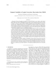
of Xie and Arkin (1997) based on gauge observations together with a variety of satellite observations. To examine seasonal and interannual modes of variability, we adopt the methodology of Ruiz-Barradas et al. (2000) and carry out rotated principal component analyses. In these analyses, three variables, SST, and zonal and meridional wind stress for each model integration (not the ensemble average), are combined into one matrix to calculate the principal components using singular value decomposition. The first 10 eigenvectors are rotated using the maximum variance procedure called VARIMAX [the International Mathematical and Statistical Library; IMSL (1989)]. Finally, linear regression on the principal component time series is used to obtain additional correlated variables such as surface heat flux, latent heat, etc. Each variable is normalized by the square root of the spatially integrated temporal variance following Nigam and Shen (1993). Before normalizing anomalies, an area weighting of the anomalies is done following Chung and Nigam (1999) in order to avoid overemphasizing the variability in the high-griddensity areas. The stability of the analysis is examined by repeating it using the full 50 yr of the NSIPP simulation and by comparison with observations. The corresponding principal components can easily be identified in all datasets. 3. Mean and seasonal cycle Climate variability contains a strong seasonal component in the tropical Atlantic. Here we begin by examining the model representation of the time mean state and its seasonal cycle. a. Mean It is evident from Fig. 1 that most of the time mean errors lie outside the equatorial area with an overestimation of wind stress in all simulations except UKMO. However, the simulated 10-m winds are in reasonable agreement with observational data except for those generated by the Japan Meteorological Agency (JMA) model which underestimates the winds in the southern Tropics (figure not shown). Thus we conclude the wind stress errors in the simulations are due to the different drag coefficients used in each model. The errors in latent heat also show systematic overestimation in most of the simulations. The errors in the time mean net shortwave radiation (Fig. 2) are 10–40 W m 22 . In contrast to the systematic errors in latent heat, the errors in shortwave radiation vary among models. ECMWF, JMA and the National Centers for Environmental Prediction (NCEP) are low while the remainder are high. Annual mean rainfall (figure not shown) also shows significant error. The simulations show stronger rainfall between the equator and 108S in the western and central basin (the region of the SITCZ) than observed either in
3861
the Xie–Arkin analysis or in COADS. The error in NCEP and NCAR exceeds 3 mm day 21 while the error in UKMO is much weaker. In the northern Tropics the simulations show reduced rainfall by up to 3 mm day 21 . This reduced rainfall is consistent with a 30% reduction in observed patterns of surface convergence and divergence throughout the Tropics (figure not shown). In particular, the subsidence region in the tropical southwest is too weak, consistent with the excess rainfall there. Interestingly, Gates et al. (1999) found excess zonal mean rainfall at almost all latitudes in the AMIP-I simulations. Net surface heat loss (figure not shown) is also overestimated in most simulations with the most severe overestimation in NCEP (generally exceeding 50 W m 22 ). Within the equatorial band the problem is reduced, with most simulations showing latent heat fluxes within 10– 30 W m 22 of COADS (the errors in COADS fluxes are discussed in Gleckler and Weare 1997). Indeed, this result is consistent with results presented in Chang et al. (2000) for CCM3 and Taylor (2000), see their Fig. 2.3). b. Seasonal cycle In our examination of surface winds we emphasize slow variations in the seasonal cycle by presenting a rotated principal component analysis on the full monthly data. The first mode representing the annual cycle explains between 40% and 59% of the wind variance. The wind stress patterns are quite similar among simulations, although generally stronger than observed (by ;0.25 dyn cm 22 ). The exception is ECMWF, which shows weaker northeast trades between 108 and 308N. The principal component time series are virtually identical in each simulation (Fig. 3). Along the equator the zonal component of the trade winds has a stronger annual cycle than observed in virtually every simulation (Fig. 4). For NCEP the mean zonal component (not shown) is 50% too strong indicating a zonal pressure gradient that is 50% too large. We suspect that this in turn may result from problems in representing convection over the adjacent continents. The meridional wind components for all simulations agree more closely with observations. An examination of the annual averaged horizontal momentum balance shows that the pressure gradient terms are larger in the simulations than in COADS (Fig. 5) while friction in the simulations varies by a factor of 2 from NSIPP (low) to JMA (high). The observed seasonal change of precipitation reaches its maximum between the equator and 108N, reflecting the north–south shift of the ITCZ. Most of the simulations show a weaker seasonal change than observed along the northwest coast of Africa, the tropical coast of Brazil (JMA, NCAR, and NSIPP) and in the central equatorial basin (ECMWF and NCEP). Next we consider seasonal changes in surface flux.
3862
JOURNAL OF CLIMATE
VOLUME 16
FIG. 1. (upper left) Annual mean surface wind stress (vectors) and latent heat flux out of ocean (contours) based on COADS observations (da Silva et al. 1994) and (other panels) the difference between specific model simulations and observations. Units are W m 22 for latent heat and dyn cm 22 for wind stress. Contour interval is 20 W m 22 for latent heat. Differences larger than 30 W m 22 are shaded. Wind stress vector scale (dyn cm 22 ) is given. Only wind stress differences larger than 0.2 dyn cm 22 in amplitude are plotted.
1 DECEMBER 2003
WANG AND CARTON
3863
FIG. 2. (upper left) Annual mean observed net shortwave radiation and differences between specific model simulated and observed. Units are W m 22 . Values larger than 630 W m 22 are shaded.
3864
JOURNAL OF CLIMATE
VOLUME 16
FIG. 3. Combined rotated principal component analysis of wind stress and SST. Here we display the first principal component (retaining the seasonal cycle). (upper) SST and wind stress (TAU) from observations. Other panels show differences between first principal component patterns. Units are 8C for SST and dyn cm 22 for wind stress. Only wind stress anomalies exceeding 0.1 dyn cm 22 are plotted. Explained variances of the observations and simulations are shown in parentheses.
1 DECEMBER 2003
WANG AND CARTON
FIG. 4. Time series of 6-month running averaged zonal (taux) and meridional (tauy) wind stress, averaged in an equatorial band (68S– 68N). Units are dyn cm 22 . Solid line is for COADS, dashed line is the average for the six simulations.
The observed seasonal change of net shortwave radiation increases from the equator to midlatitude in both hemispheres. All simulations show a weaker seasonal change than observed in both equatorial and tropical regions. Among them, ECMWF, NCEP, and UKMO have a much weaker seasonal change in the northern Tropics. NCAR and NSIPP have the closest pattern to the observations. The observed seasonal change of latent heat reaches its maximum amplitude in the latitude band between 108 and 208 in both hemispheres (Fig. 6). In boreal summer the southeast trades intensify, leading to an increase in evaporation and latent heat loss in the south and a decrease in evaporation and latent heat loss in the north, while the situation is reversed in winter. All simulations except NSIPP show an overestimation of this seasonal change. The strongest overestimation occurs in ECMWF and NCEP, whose seasonal change is approximately 80% larger than COADS. Much of this difference can be accounted for by the differences in the seasonal changes of surface humidity (e.g., the seasonal changes of surface humidity in the northern Tropics in ECMWF and NCEP are the strongest among all models). 4. Interannual variability As evident in Fig. 4, surface winds have significant interannual variability. Here we address this variability by repeating the rotated principal component analysis over the same 17-yr record for each simulation and for COADS with the seasonal cycle removed from the original data. In each analysis we identify the atmospheric patterns associated with the Atlantic Nin˜o and interhemispheric modes discussed in the introduction. As will be seen from comparison of the associated time series, the identification is quite clear leaving little room for subjectivity. We examine the stability of the patterns
3865
FIG. 5. Magnitudes of terms in the time mean horizontal momentum equation (following Deser 1993; Li and Wang 1994) averaged over 208S–308N at 1000 mb. Friction is calculated as the residual. Seasonal and interannual changes are ;5%–10%. Unit is 10–5 m s 22 .
using the longer 50-yr time series from NSIPP and COADS observations. The principal components of wind stress for both patterns are presented in Figs. 7 and 8, with corresponding time series showing the similarity of the components in Fig. 9. The first pattern we consider corresponds to the Atlantic Nin˜o (Figs. 7 and 9) whose explained variances range from 14% to 17%, slightly stronger than observed during this period (12%). An examination of the seasonality of this pattern shows that for all simulations the maximum explained variance occurs in boreal summer, consistent with COADS. All simulations show a relaxation of the equatorial trade wind stress in the west by .0.1 dyn cm 22 . Most simulations show strengthening of the southeast trade winds in the southeast, consistent with an enhancement of the North African monsoon, and the northeast trade winds in the north, reflecting a strengthening of the summer subtropical high pressure system. We also note that the observed wind stress anomalies in the southern Tropics are less coherent than in the models. This is probably due to the sparse observational data in this region. The shift in the surface winds is reflected in a southward shift and intensification of diabatic heating as well as precipitation (Fig. 10) The strongest precipitation anomalies, along with the most intense westerly wind anomalies occur in three simulations: JMA, UKMO, and NCEP. In contrast, ECMWF and NSIPP have relatively weak wind and precipitation anomalies, but closer to those of COADS. The second pattern we consider corresponds to the dipolelike interhemispheric mode. The surface wind field shows a strong cross-equatorial component blowing onto a warm Northern Hemisphere in response to warming SSTs in the northern Tropics, with a relaxation of the northeast trade winds and a weaker strengthening of the southeast trade winds (Fig. 8). The simulations also reveal a pattern of surface winds similar to that
3866
JOURNAL OF CLIMATE
VOLUME 16
FIG. 6. Climatological seasonal change (Jun–Aug mean minus Dec– Feb mean) of latent heat in (upper left) observations and (other panels) simulations. Contour intervals are 20 W m 22 . Values larger than 640 W m 22 are shaded.
1 DECEMBER 2003
WANG AND CARTON
3867
FIG. 7. Wind stress anomalies of Atlantic Nin˜o mode from principal component analysis of Jun–Aug data on the rotated time coefficient of this mode. Units are dyn cm 22 for wind stress. Only wind stress values larger than 0.02 dyn cm 22 in amplitude are plotted. Explained variances are shown in parentheses.
3868
JOURNAL OF CLIMATE
VOLUME 16
FIG. 8. Wind stress anomalies (vectors) of interhemispheric mode from principal component analysis of MAM data and regression of latent heat (contours) on the rotated time coefficient of this mode. Units are dyn cm 22 for wind stress. Contour interval for latent heat is 4 W m 22 and zero contours are not drawn. Latent heat anomalies larger than 66 W m 22 are shaded. Positive values indicate the ocean gains heat. Only wind stress values larger than 0.02 dyn cm 22 in amplitude are plotted. Explained variances are shown in parentheses.
1 DECEMBER 2003
WANG AND CARTON
3869
FIG. 9. Time coefficients for the (bottom) Atlantic Nin˜ o and (top) interhemispheric patterns in their strongest seasons.
observed in the region of the equator and the southern trade wind zones with explained variances ranging from 11% to 13%, slightly less than observed during this period (15%). In the northern trade wind zones, ECMWF and NSIPP have similar surface wind patterns to that observed while the remaining show significant differences with respect to COADS. The weakest wind anomalies, significantly weaker than observed, occur in three simulations: JMA, UKMO, and NSIPP. An examination of the seasonality of this pattern shows that all simulations have maximum explained variance in boreal spring [March–April–May (MAM)], in agreement with COADS. The northward shift of the trade wind systems and the ITCZ causes drying in the southwest Tropics and enhanced precipitation in the northwest (Fig. 11). The weakest precipitation patterns associated with the interhemispheric mode are produced by ECMWF and NSIPP, which are significantly weaker than observed. Indeed, only NCEP and NCAR have precipitation anomalies as large as observed. These two simulations also have the strongest interhemispheric wind anomalies. Latent heat flux anomalies associated with the interhemispheric patterns are the most important term driving decadal SST variations in this region (Carton et al. 1996). Since anomalous SST associated with the positive phase of the interhemispheric mode is positive throughout the northern Tropics, a reduced anomalous latent heat flux in the northern Tropics corresponds to positive feedback between the atmosphere and ocean, while an increase in anomalous latent heat flux corresponds to negative feedback. In the Southern Hemi-
sphere the anomalous SST is weakly negative, and thus the correspondence between the sign of the latent heat flux and the feedback is reversed. As discussed in the introduction, an earlier examination of the NCAR CCM3 (Chang et al. 2000) pointed out the presence of a zone of positive feedback in the western Tropics and negative feedback in the east (also evident in Fig. 8). We find similar behavior in four of the remaining simulations: NCAR, NCEP, UKMO, and ECMWF. All four differ from COADS, which shows an expanded region of positive feedback and little negative feedback. In the other two simulations, JMA and NSIPP, a broad region of negative feedback is evident, with no corresponding region of positive feedback. Interannual variations in latent heat flux may arise from fluctuations in wind forcing or fluctuations in relative humidity: LH9 5 r a LC e ( | U | 9d q 1 | U | dq).
(1)
Overbars and primes indicate climatological seasonal values and deviations from climatological seasonal values. Here L is the latent heat of evaporation, r a the air density, C e the transfer coefficient (set to 1.2 3 10 23 ), | U | the wind speed at 10-m height, and d q is the difference between specific humidity and saturation-specific humidity. Thus (1) represents a linear decomposition into anomalous wind-driven and anomalous humidity-driven latent heat flux components. The observed anomalous wind-driven component dominates the humidity-driven component over much of the ocean, reversing sign in the Southern Hemisphere (Figs. 12 and 13). Because the SST anomaly associated with the in-
3870
JOURNAL OF CLIMATE
VOLUME 16
FIG. 10. Regression of precipitation on the rotated time series of the Atlantic Nin˜o mode for Jun–Aug. Contour interval is 0.4 mm day 21 . Zero contours are not drawn. (upper left) Observed precipitation data.
1 DECEMBER 2003
WANG AND CARTON
3871
FIG. 11. Same as Fig. 10, except for the interhemispheric mode of MAM.
3872
JOURNAL OF CLIMATE
VOLUME 16
FIG. 12. Regression of the wind-driven components of latent heat [see (1)] on the time series of the interhemispheric pattern of MAM for each data source. Units are W m 22 .
terhemispheric pattern also reverses sign in the Southern Hemisphere, the wind-driven latent heat flux component acts in the positive feedback sense of enhancing initial SST anomalies in both hemispheres. The humidity-driv-
en component predominates along the coast of northwest South America and in the southern central basin. In contrast the simulations show only weak zones of positive feedback associated with wind-driven latent
1 DECEMBER 2003
WANG AND CARTON
3873
FIG. 13. Regression of the humidity-driven components of latent heat [see (1)] on the rotated time coefficient of the interhemispheric pattern of MAM for each data source. Units are W m 22 .
heat flux because of the relatively weak wind anomalies associated with the interhemispheric pattern and because of the strong seasonal cycle of relative humidity in the boundary layer over much of the basin. The largest zone
of positive feedback occurs in UKMO, while JMA has no positive feedback. The humidity-driven component is larger than observed for most simulations, but is large mainly in the northeast and acts as a negative feedback.
3874
JOURNAL OF CLIMATE
In applying these results to coupled air–sea interaction the reader is reminded that in these experiments the ocean acts as an infinite heat reservoir because SST is specified. Thus, as a reviewer points out, this will give misleading results in situations where in reality SST is being determined by atmospheric effects (one-way driving). We suspect the discrepancy between the observed and simulated humidity-driven component of latent heat flux is related to the simulated error in the boundary layer humidity over the African continent. Interestingly, an apparently related model error in simulating ENSO surface fluxes has been pointed out by Kleeman et al. (2001). The stability of our estimate of the interhemispheric pattern is examined by repeating the analysis using 50yr records available for the NCEP–NCAR reanalysis and the NSIPP simulation. The observed and NSIPP interhemispheric patterns are weaker when calculated using this extended data set by 30%–40%, but the tendencies of the anomalies are quite similar. 5. Conclusions The tropical Atlantic Ocean occupies a narrow basin surrounded by continents supporting zones of intense convection as well as subsidence. These patterns strongly influence the mean circulation and likely influence year-to-year variability as well. The position and intensity of convection over the ocean is sensitive to yearto-year changes in SST. The atmospheric boundary layer also responds to SST gradients that are stronger than in the other tropical oceans. In order to understand how the atmosphere responds to year-to-year fluctuations in SST we have examined the 17-yr-long simulations of six atmospheric general circulation models in the tropical Atlantic sector in comparison with COADS surface observations. Five of these models were obtained from the Atmospheric Model Intercomparison Project, while a sixth and longer 50-yr simulation was obtained from the NASA Seasonal to Interannual Prediction Project. The models differ in important ways including horizontal and vertical resolution, convective schemes, and cumulus parameterization. Because of the potential interaction with year-to-year changes, we begin by examining the time mean and seasonal cycles. We find that most simulations overestimate the time mean wind stress outside of the Tropics. However, this is largely due to differences in surface drag parameterization. Along the equator the seasonal cycle in surface wind stress is somewhat exaggerated, most severely in UKMO, while the zonal component of NCEP is too intense by 0.2 dyn cm 22 . We find weak wind convergence and underestimation of precipitation between the equator and 108S in the western and central basin as well as the northern Tropics. Along the equator the seasonal cycle in surface wind stress is somewhat exaggerated, most severely in UKMO.
VOLUME 16
At longer interannual and decadal periods the tropical Atlantic appears to support a variety of modes including an Atlantic Nin˜o which has its strongest expression in during boreal summer, and an interhemispheric mode that exhibits a dipolelike response in diabatic heating and has its strongest expression during boreal spring. Here we focus on the connection between the atmospheric response and local pattern of SST using a rotated principal component analysis. Examination of the atmospheric patterns associated with the Atlantic Nin˜o reveals that the pattern of the response to the Atlantic Nin˜o is similar among simulations and COADS although magnitudes differ. All simulations show a relaxation of the equatorial trade winds in the west. Most show a strengthening of the southeast trade winds in the southeast, consistent with an enhancement of the North African monsoon, and the northeast trade winds in the northeast, reflecting a strengthening of the summer subtropical high pressure system, as well as an equatorward shift and strengthening of precipitation. Surprisingly, three of the simulations, JMA, UKMO, and NCEP, had responses that were stronger than observed. In contrast, ECMWF and NSIPP have relatively weak wind and precipitation anomalies, more consistent with the observations. Our examination of the interhemispheric pattern shows greater diversity. In this pattern a northward shift of the trade wind systems and the ITCZ develops in response to a positive anomalous interhemispheric SST gradient, and results in drying of the southwest Tropics and enhanced precipitation in the northwest. Of the six simulations only NCEP and NCAR have precipitation and cross-equatorial wind anomalies as large as observed. The atmospheric pattern includes changes in latent heat flux, which are believed to be critical in controlling the development of anomalous SST through a positive feedback on boundary layer winds. The use of AMIPtype simulations to diagnose air–sea interaction may be misleading. Barsugli and Battisti (1998) point out that in midlatitudes, in regions where anomalous SST is being controlled by atmospheric effects, use of prescribed SST boundary condition leads to unrealistic results. Here in the Tropics, however, the coupled model results of Chang et al. (2000) suggest that the coupling between the atmosphere and ocean is sufficiently tight to avoid this problem. Acknowledgments. We gratefully acknowledge the support of the National Science Foundation (OCE9812404, OCE0113148) for this work. We would like to thank Peter Gleckler of the Program for Climate Model Diagnosis and Intercomparison at Lawrence Livermore National Laboratory for providing access to the AMIP-II dataset. All the AMIP-II participant modeling groups whose outputs are used in this work are gratefully acknowledged. We would also like to thank Max Suarez and Philip Pegion of NASA for providing NSIPP
1 DECEMBER 2003
WANG AND CARTON
model outputs to us. Two anonymous reviewers have given valuable suggestions in improving the presentation of our results. Their help is gratefully acknowledged. This work forms part of the dissertation research of JW. REFERENCES Arakawa, A., and W. H. Schubert, 1974: Interaction of cumulus cloud ensemble with the large-scale environment, Part I. J. Atmos. Sci., 31, 671–701. Barsugli, J. J., and D. S. Battisti, 1998: The basic effects of atmosphere–ocean thermal coupling on midlatitude variability. J. Atmos. Sci., 55, 477–493. Betts, A. K., and M. J. Miller, 1993: The Betts–Miller scheme. The Representation of Cumulus Convection in Numerical Models, Meteor. Monogr., No. 46, Amer. Meteor. Soc., 107–122. Bjerknes, J., 1969: Atmospheric teleconnections from the equatorial Pacific. Mon. Wea. Rev., 97, 163–172. Carton, J. A., and Z. Zhou, 1997: Annual cycle of sea surface temperature in the tropical Atlantic Ocean. J. Geophys. Res., 102, 27 813–27 824. ——, X. Cao, B. S. Giese, and A. M. da Silva, 1996: Decadal and interannual SST variability in the tropical Atlantic. J. Phys. Oceanogr., 26, 1165–1175. Chang, P., R. Saravanan, L. Ji, and G. C. Hegerl, 2000: The effect of local sea surface temperatures on atmospheric circulation over the tropical Atlantic sector. J. Climate, 13, 2195–2216. Chung, C., and S. Nigam, 1999: Weighting of geophysical data in principal component analysis. J. Geophys. Res., 104, 16 925– 16 928. Da Silva, A. M., A. C. Young, and S. Levitus, 1994: Algorithms and Procedures. Vol.1, Atlas of Surface Marine Data 1994, National Oceanic and Atmospheric Administration, 83 pp. Deser, C., 1993: Diagnosis of the surface momentum balance over the tropical Pacific Ocean. J. Climate, 6, 64–74. Ebisuzaki, W., and H. M. Van den Dool, 1993: The Atmospheric Model Intercomparison Project at the National Meteorological Center. NMC Office Note 402, 19 pp. ECMWF, 1993: The description of the ECMWF/WCRP Level III— A global atmospheric data archive. European Centre for Medium-Range Weather Forecasts, Tech. Attachment, Reading, United Kingdom, 72 pp. Enfield, D. B., and D. A. Mayer, 1997: Tropical Atlantic SST variability and its relation to El Nin˜o–South Oscillation. J. Geophys. Res., 102, 929–945. Gates, W. L., 1992: AMIP: The Atmospheric Model Intercomparison Project. Bull. Amer. Meteor. Soc., 73, 1962–1970. ——, and Coauthors, 1999: An overview of the results of the Atmospheric Model Intercomparison Project (AMIP I). Bull. Amer. Meteor. Soc., 80, 29–56. Gleckler, P. J., and B. Weare, 1997: Uncertainties in global ocean surface heat flux climatologies derived from ship observations. J. Climate, 10, 2763–2781. Gregory, D., and P. R. Rowntree, 1990: A mass flux convection scheme with representation of cloud ensemble characteristics and stability dependent closure. Mon. Wea. Rev., 118, 1483–1506. Groisman, P. Y., R. S. Bradley, and B. Sun, 2000: The relationship of cloud cover to near-surface temperature and humidity: Comparison of GCM simulations with empirical data. J. Climate, 13, 1858–1878. Grumbine, R. W., 1996: Automated passive microwave sea ice concentration analysis at NCEP. NOAA Tech. Note 120, 13 pp. Hack, J. J., 1994: Parameterization of moist convection in the National Center for Atmospheric Research Community Climate Model (CCM2). J. Geophys. Res., 99, 5551–5568. Hastenrath, S., 1991: Climate Dynamics of the Tropics. Kluwer Academic, 488 pp.
3875
IMSL, 1989: International Mathematical and Statistical Library Version 1.1. IMSL Publications. Kiehl, J. T., J. J. Hack, G. B. Bonan, B. A. Boville, D. L. Williamson, and P. J. Rasch, 1998: The National Center for Atmospheric Research Community Climate Model: CCM3. J. Climate, 11, 1131–1150. Kirtman, B. P., and D. G. DeWitt, 1997: Comparison of atmospheric model wind stress with three different convective parameterizations: Sensitivity of tropical Pacific Ocean simulations. Mon. Wea. Rev., 125, 1231–1250. Kleeman, R., G. Wang, and S. Jewson, 2001: Surface flux response to interannual tropical Pacific sea surface temperature variability in AMIP models. Climate Dyn., 17, 627–641. Kuo, H. L., 1974: Further studies of the parameterization of the influence of cumulus convection on large-scale flow. J. Atmos. Sci., 31, 1232–1240. Lau, K. M., J. H. Kim, and Y. Sud, 1996: Intercomparison of hydrologic processes in AMIP GCMs. Bull. Amer. Meteor. Soc., 77, 2209–2227. Li, T., and B. Wang, 1994: A thermodynamic equilibrium climate model for monthly mean surface winds and precipitation over the tropical Pacific. J. Atmos. Sci., 51, 1372–1385. Lin, J. W. B., and J. D. Neelin, 2000: Influence of a stochastic moist convective parameterization on tropical climate variability. Geophys. Res. Lett., 27, 3691–3694. Maloney, E. D., and D. L. Hartmann, 2001: The sensitivity of intraseasonal variability in the NCAR CCM3 to changes in convective parameterization. J. Climate, 14, 2015–2034. Nigam, S., and H.-S. Shen, 1993: Structure of oceanic and atmospheric low-frequency variability over the tropical Pacific and Indian Oceans. Part I: COADS observations. J. Climate, 7, 1750–1771. Nomura, A., 1995: Global sea-ice concentration data set for use in the ECMWF re-analysis system. ECMWF Tech. Rep. 76, 40 pp. Numerical Prediction Division, 1997: Outline of the Operational Numerical Weather Prediction at the Japan Meteorological Agency. Japan Meteorological Society, Tokyo, Japan, 126 pp. Philander, S. G. H., 1990: El Nin˜o, La Nin˜o, and the Southern Oscillation. Academic Press, 293 pp. ——, and R. C. Pacanowski, 1986: A model of the seasonal cycle in the tropical Atlantic Ocean. J. Geophys. Res., 91, 14 192–14 206. Phillips, T. J., 1996: Documentation of the AMIP models on the World Wide Web. Bull. Amer. Meteor. Soc., 77, 1191–1196. Pope, V. D., M. L. Gallani, P. R. Rowntree, and R. A. Stratton, 2000: The impact of new physical parameterizations in the Hadley Centre climate model: HadAM3. Climate Dyn., 16, 123–146. Rayner, N. A., D. E. Parker, E. B. Horton, C. K. Folland, L. V. Alexander, D. P. Rowell, E. C. Kent, and A. Kaplan, 2003: Global analyses of sea surface temperature, sea ice, and night marine air temperature since the late nineteenth century. J. Geophys. Res., 108, 4407, doi:10.1029/2002JD002670. Reynolds, R. W., and T. M. Smith., 1994: Improved global sea surface temperature analysis using optimum interpolation. J. Climate, 7, 929–948. Robock, A., C. A. Schlosser, K. Ya. Vinnokov, N. A. Speranskaya, J. K. Entin, and S. Qiu, 1998: Evaluation of AMIP soil moisture simulations. Global Planet. Change, 19, 181–208. Ruiz-Barradas, A., J. A. Carton, and S. Nigam, 2000: Structure of interannual-to-decadal climate variability in the tropical Atlantic sector. J. Climate, 13, 3285–3297. Saji, N. H., and B. N. Goswami, 1997: Intercomparison of the seasonal cycle of tropical surface stress in 17 AMIP atmospheric general circulation models. Climate Dyn., 13, 561–585. Sperber, K. R., and T. Palmer, 1996: Interannual tropical rainfall variability in general circulation model simulations associated with the Atmospheric Model Intercomparison Project. J. Climate, 9, 2727–2750. Srinivasan, G., M. Hulme, and C. G. Jones, 1995: An evaluation of the spatial and interannual variability of the tropical precipitation as simulated by GCMs. Geophys. Res. Lett., 22, 1697–1700.
3876
JOURNAL OF CLIMATE
Suarez, M. J., and L. L. Takacs, 1995: Documentation of the ARIES/ GOES Dynamic Core: Version 2. NASA Tech. Memo. 104606, Vol. 5, 45 pp. [Available from NASA Center for Aerospace Information, 800 Elkridge Landing Rd., Linthicum Heights, MD 21090-2934.] Sutton, R. T., S. P. Jewson, and D. P. Rodwell, 2000: The elements of climate variability in the tropical Atlantic region. J. Climate, 13, 3261–3284. Taylor, P. K., Ed., 2000: Intercomparison and validation of ocean– atmosphere energy flux fields. Joint WCRP/SCOR Working Group on Air–Sea Fluxes Final Rep. WCRP-112, WMO/TD-No. 1036, 306 pp. Tiedtke, M., W. A. Heckley, and J. Slingo, 1988: Tropical forecasting at ECMWF—The influence of physical parameterization on the mean structure of forecasts and analyses. Quart. J. Roy. Meteor. Soc., 114, 639–664. Weare, B. C., and I. Mokhov, 1995: Evaluation of total cloudiness and its variability in the Atmospheric Model Intercomparison Project. J. Climate, 8, 2224–2238. ——, and AMIP Modeling Groups, 1996: Evaluation of the vertical
VOLUME 16
structure of zonally averaged cloudiness and its variability in the Atmospheric Model Intercomparison Project. J. Climate, 9, 3419–3431. Wolter, K., 1997: Trimming problems and remedies in COADS. J. Climate, 10, 1980–1997. Wu, X. Q., and M. W. Moncrieff, 2001: Sensitivity of single column model solutions to convective parameterizations and initial conditions. J. Climate, 14, 2563–2582. Xie, P., and P. A. Arkin, 1997: Global precipitation: A 17-year monthly analysis based on gauge observations, satellite estimations, and numerical model outputs. Bull. Amer. Meteor. Soc., 78, 2539–2558. Zebiak, S. E., 1993: Air–sea interaction in the equatorial Atlantic region. J. Climate, 6, 1567–1586. Zhang, G. J., 1995: The sensitivity of surface-energy balance to convective parameterization in a general circulation model. J. Atmos. Sci., 52, 1370–1382. ——, and N. A. McFarlane, 1995: Sensitivity of climate simulation to the parameterization of cumulus convection in the Canadian Climate Centre General Circulation Model. Atmos.–Ocean, 33, 407–446.