EMILIO A. LACA. A stochastic dynamic programming model for extensive livestock systems is developed. The model optimizes sales/retention decisions when ...
Modeling Extensive Livestock Production Systems: An Application to Sheep Production in Kazakhstan
Mimako Kobayashi, Richard E. Howitt, Lovell S. Jarvis and Emilio A. Laca University of California, Davis
Paper prepared for presentation at the American Agricultural Economics Association Annual Meeting, Montreal, Canada, July 27-30, 2003
Copyright 2003 by Kobayashi, Howitt, Jarvis, and Laca. All rights reserved. Readers may make verbatim copies of this document for non-commercial purposes by any means, provided that this copyright notice appears on all such copies.
MODELING EXTENSIVE LIVESTOCK PRODUCTION SYSTEMS: AN APPLICATION TO SHEEP PRODUCTION IN KAZAKHSTAN MIMAKO KOBAYASHI, RICHARD E. HOWITT, LOVELL S. JARVIS, AND EMILIO A. LACA
A stochastic dynamic programming model for extensive livestock systems is developed. The model optimizes sales/retention decisions when future forage production, which affects animal performance and hence profitability, is uncertain. The model is applied to sheep production in Kazakhstan to evaluate policy alternatives. Key words:
stochastic dynamic programming, extensive livestock production, Kazakhstan, transition economies
Mimako Kobayashi is a graduate student, and Richard E. Howitt and Lovell S. Jarvis are professors, Department of Agricultural and Resource Economics, University of California, Davis, and Emilio A. Laca is an associate professor, Department of Agronomy and Range Science, University of California, Davis. This publication was made possible through support provided by US Universities, host country institutions and the Office of Agriculture and Food Security, Global Bureau, US Agency for International Development, under Grant No. PCE-G-98-00036-00. The opinions expressed herein are those of the author(s) and do not necessarily reflect the views of USAID. This research was sponsored by the Global Livestock CRSP, Management Entity, University of California, Davis.
1.
Introduction In many countries, sheep and cattle production are based on extensive technology
where animals graze natural or cultivated pastures rather than being intensively fed with supplements.
In such a system, animal productivity is strongly affected by forage
production, which in turn depends largely on climatic conditions.
Producers are
inherently at risk from climatic fluctuations, and this risk is greater the greater the costs of supplementary feeding. Scientists have documented and analyzed the impacts of climatic fluctuations on production both at the animal and producer levels. However, in order to better understand the intrinsic dynamics and stochastic nature of extensive livestock production, a comprehensive bio-economic analytic tool is needed. Stochastic dynamic programming models have been used to solve for optimal strategies when uncertainty is involved in livestock production, but such models have been applied to limited decisions of livestock production (e.g., stocking rate, culling). Various types of biological simulation models have also been used to analyze extensive livestock production, but most such models assume fixed decision rules (e.g., a fixed offtake rate) that limit the economic insights that can be gained. In this paper, we develop a bio-economic mathematical programming model that incorporates animal population dynamics and biology, forage stochasticity and grazing, and producer decision making. More specifically, we extend the technique developed by Howitt et al. (2002) of value function approximation in stochastic dynamic programming (SDP) and simulation based on the value function thus obtained. This approach reduces the computational difficulty of incorporating multiple state variables, which we believe has hampered development of suitable analytic tools for extensive livestock production
1
systems. Our current model contains five state variables and a single stochastic factor. The model’s results provide greater information about, and thus insight into, the tradeoffs that producers face when making decisions about sales vs. retention of different types of animals where future animal performance is uncertain (in terms of animal productivity, fertility and mortality) due to fluctuations in future pasture conditions. The model also allows us to analyze the impact of risk aversion on sales/retention decisions. We apply the model to sheep production in Kazakhstan, a former Soviet Union (FSU) republic. Sheep production has always been an important part of the traditionally nomadic economy. During the Soviet period, heavy subsidies were used to increase sheep flocks and wool and mutton production, much of which was exported to the other FSU republics.
Production was concentrated on large-scale state and collective farms.
During the last decade of transition from a centrally planned to a market economy, Kazakhstan’s sheep production has gone through major structural changes. Following price liberalization, input subsidies and output price supports were removed, and livestock production became largely unprofitable. As supplementary feeding became no longer profitable, producers had to rely primarily on natural pastures, which produce little nutrition during the winter. The timing of Kazakhstan’s transition corresponded the collapse of the world wool market in 1991. In response, Kazakhstan’s sheep population and production declined sharply, especially on the large state and collective farms and the large private enterprises that succeeded them. With the low price of wool, wool-type breeds were slaughtered faster, and meat/fat type breeds became dominant. Overall, the sheep population in Kazakhstan declined by 70% during the first decade of transition.
2
During the process of privatization of former state and collective farms, many farm assets, including animals, were distributed to member workers and sheep production was fragmented into numerous small units.
Currently, small subsistence producers
account for the vast majority of sheep flock and output in Kazakhstan. However, as restructuring and development progress, it is likely that medium-sized individual commercial operations will become more important. Transition in Kazakhstan is an ongoing process, and agricultural policies are adjusted dynamically. Our model, as a component of a larger project, aims at determining how Kazakhstan’s sheep sector can be restructured given the observed changes during the first decade of transition. How can mid-sized commercial producers be promoted? What kind of constraints do they face? What types of policy measures will be effective now that the production is, and likely continues to be given relative prices, largely based on extensive rangeland grazing? Current government policy does not seem fully consistent with the market shift for the Kazakhstan’s sheep sector. The emphasis seems to be on the reintroduction of purebred animals that were lost in the course of disorganized decollectivization. The government attributes the current low productivity (in terms of meat per head and wool or milk per head) to the loss of Soviet breeds. However, we believe that producers may have shifted from purebred to locally adapted, hybrid animals because the latter are more robust to production conditions, including a relatively low management input and limited nutrition. Soviet purebred animals may be capable of producing a higher output per unit under sharply improved production conditions, but they likely are not as profitable in the current production environment. Breed control will become important as Kazakhstan becomes once again a meat and wool exporter and tighter controls of output quality are
3
required. However, both internal and external markets have changed, and the mere reintroduction of the Soviet breeds may not be consistent with today’s market demand. We hypothesize that low-cost extensive production will be more efficient than Sovietstyle intensive production, at least for the foreseeable future. We also hypothesize that the increased availability of supplementary feed during the harsh winter (when grazing is not possible) will reduce risk and improve producer welfare. The analytical framework used this paper is suitable for addressing these types of policy questions. We believe that the dominant characteristic of extensive livestock production is the stochastic nature of pasture production and the optimization of livestock herd management over stochastic forage availability. Policies must take into account the nature of the extremely difficult setting in which producers must make decisions. The necessity of modeling stochastic forage production is even greater in developing countries, where supplementary feeding is unavailable or very expensive. A comprehensive analysis of the sheep production in Kazakhstan is outside of the scope of this paper. Here, our discussion will demonstrate the model’s function and its applicability to this class of economic problem through its application to a specific region in Kazakhstan. The paper is organized as follows. In Section 2, the model structure, together with characteristics of sheep production in Kazakhstan, is outlined. In Section 3, we present selected simulation results. In Section 4, we discuss the usefulness and limitation of our approach.
2.
Model specification and methodology
General setting:
4
We model a private producer who grazes his sheep in a fixed grazing area of private property. The institution of sheep herding in Kazakhstan is essentially, but not officially, compatible with this assumption. In present day Kazakhstan, most agricultural lands are still in the state’s ownership, but land use rights are defined and allocated to individuals and groups of individuals in the form of state leases. 1 Commercial-scale individual producers tend to lease traditional grazing areas remote from human settlements.
On the other hand, subsistence-scale livestock holders tend to use
“communal” grazing areas located near the settlements. The customary arrangement is that any individuals from the community can use the communal grazing lands (open access regime). However, neighbors or families typically pool their livestock and graze jointly (they either take turns in herding or choose a designated herder and pay for his labor).
Thus the range management by subsistence-scale producers resembles
cooperation at the communal pasture level. Local scientists claim that such communal lands suffer from overgrazing as the majority of livestock are held by subsistence producers, who tend to stay close to the settlements. On the other hand, remote pastures, which are often no longer stocked because the collectives’ animal production has almost vanished, have started to recover from past (Soviet) overgrazing. In our model, however, we do not consider long-term interactions between grazing intensity and forage production. Instead, we consider a “medium-run” situation where forage production fluctuates from year to year around a stationary mean. This assumption would be valid if some producers move their sheep to
1
General agreement has been reached for privatization of croplands. However, given the nomadic history with no experience of private ownership of pasturelands, pastureland policy has lagged behind.
5
remote pastures once congestion is felt on communal pastures. At the current level of livestock population, congestion in the remote pastures is unlikely. The producer is assumed to maximize the future stream of expected net revenue of sheep production (animal and wool sales). He takes sheep biology, forage production, and input and output prices as given. He observes the current state of flock size, animal condition, and forage availability, and in turn chooses how many animals to sell (or retain over the winter) and how much supplements to feed during winter. production is unknown.
Future forage
Only the probability distribution of forage production is
assumed to be known to the producer. Sales/retention decisions affect current and future meat output by changing flock size and composition, which in turn affects the reproduction rate. Thus, flock management resembles a series of asset portfolio choices (Jarvis 1974). The flock size decision also affects stocking density on pastures and forage availability per head. Flock size is also interrelated with winter feeding decisions since producers must incur larger feeding costs if they are to carry more livestock through the winter. Feeding decisions in turn affect future animal productivity and flock size, through births and deaths. Model specifications and assumptions: Following the sheep production practices commonly observed in southeastern Kazakhstan, the main sheep producing area of the country, we assume the timing of events during a year occurs as in Figure 1. First, we define the “production” year to start in early spring, when forage production and lambing take place. We assume shearing occurs once a year in May. Grazing is possible through spring, summer, and fall, and grass hay and barley are the only source of nutrient intake during winter. Animal sales
6
take place in fall, when the animals are typically in the best condition. Breeding takes place in fall, and lambing in early spring after five-month gestation period.
For
traceability, we assume that all deaths occur in winter (lamb mortality occurs between lambing and weaning in summer). We treat the production year (from spring to spring) as the basic time unit, which will be indexed as t, t+1, and so on. Forage production, producer decision making, and changes in the sheep flock size are all assumed to take place once a year, that is, seasons within a year are not modeled explicitly. Based on the above assumptions on sheep management, we now define forage production, sheep biology, and revenues and costs, in mathematical expressions. (a)
Forage production Forage production on Kazakhstan’s natural pastures fluctuates from year to year
as rainfall fluctuates (Robinson, Milner-Gulland, and Alimaev 2003). To determine the distribution of forage production in the area, we used the annual forage biomass data found in Robinson, Milner-Gulland, and Alimaev (2003) for three locations in southeastern Kazakhstan. Forage production data from other sources suggest that the average annual forage biomass produced in our study area is about 470 kg/ha (dry matter). The gamma distribution with parameters (3.24, 145.3) was found to fit the available information most closely. We consider a hypothetical 10,000 ha pasture on which annual total forage production per hectare (FPRODt) occurs according to the above gamma distribution. We assume that the grazing area is exclusively used by the sheep flock (no entry by other flocks, other livestock, or wild animals).
7
(b)
Sheep biology In modeling the sheep biology dynamics, we keep track of year-to-year changes
in the number of animals in different age/sex categories and animal body condition. We denote newborn (0-year-old) female and male lambs as LAFt and LAMt, respectively. Lambs grow into yearlings in the following year (YRFt and YRMt for female and male yearlings, respectively). For simplicity, we treat adult sheep (two years and older) for each sex as a group: ewes (EWEt) and wethers (WETt). We do not consider rams because ram management is usually not a significant part of a farmer’s concern. The body condition of individual animals changes continuously throughout the year due to feed intake and animal health, and body condition affect biological outcomes such as births and deaths. Under the discrete-time assumption, we need to compound the continuous changes into discrete annual changes. Also, for traceability, we need to take a representative animal from each age/sex group and monitor their body condition. Given technical limitations and to save dimensionality, we adopt the bodyweight of an average ewe (BWt) as the only indicator of animal body condition for the entire flock. Implicitly we assume that the body condition of all sheep in the flock (not just ewes) will change in proportion to that of the representative ewe.
This assumption can lead to extreme
predictions in some cases. For example, if the representative ewe’s mortality rate is 1.0, then the entire model flock will die, even though there would be survivors in a real flock with the same average characteristics. We will address this problem below as we discuss the specifications of individual equations. Another assumption is that the dynamics of a ewe’s bodyweight can be represented by a Markov process, i.e., all the information for past controls is
8
characterized in the current state level. However, longer lagged effects may occur in animal biology. For example, the impact of bad feeding in one year may not be entirely reversed by simply feeding well in the following year. Therefore, some biological relationships used in the present model for economic analyses are simplifications of the “true” relationships. All the simplified biological equations in this sub-section are derived from a more detailed, single-animal, daily-based sheep simulation model (XLUMBE) developed by Laca. More specifically, we first ran XLUMBE with changing input parameters (grazing, feeding, and body fat content) and generated output data on bodyweight, birth and mortality rates, and wool production (aggregated into annual data). Using the generated data, we then estimated the parameters of simplified biological equations.
Since
statistical properties are irrelevant, we used least squares estimation for all equations. We discuss the specification of each biological equation below.
Table 1 provides the
parameter estimates, together with the R2 values and the number of data points used (n). XLUMBE was parameterized for Kazakh Fine Wool (KFW) sheep for the data generated for this paper. We will repeat the procedure for Kazakh Fat Tail (KFT) breed in the future. (These are the main wool and meat/fat type breeds observed in Kazakhstan.) < Nutrient intake > Individual animals are assumed to graze freely every day, but the amount one animal can graze is determined by forage production (more abundant, palatable and nutritious forage tend to allow greater intake), the size of the animal (larger animals have greater energy demand and appetite), as well as how many animals are put on the same
9
pasture (stocking density). We assume the following translog relationship in predicting forage intake per ewe (FORAGEt): (1)
lnFORAGEt = α0 + α1lnFPRODt + α2lnTOTGRAZEt + α3lnBWt + α4lnFPRODt2 + α5lnTOTGRAZEt2 + α6lnBWt2 + α7lnFPRODt*lnTOTGRAZEt + α8lnFPRODt*lnBWt + α9lnTOTGRAZEt*lnBWt
where TOTGRAZEt is the total number of animals to graze in “ewe unit” defined as: (2)
TOTGRAZEt = 0.2(1 – δLAt)(LAFt + LAMt) + 0.7(YRFt + YRMt) + EWEt + WETt
and δLAt is the lamb mortality rate (below). Note that the information about the pasture acreage (10,000 ha here) is embedded in the forage equation parameters. We consider supplementary feeding of grass hay and barley during winter (for 127 days in XLUMBE). We denote the amount of grass hay and barley fed per head of ewe unit during winter as GHAYt and BARt, respectively. For simplicity, we assume that proportionate amounts would be fed to other age/sex categories, although different categories or individual animals may receive different amount in practice. The total number of animals in ewe unit to be fed during winter is defined as: (3)
TOTFEDt = 0.3(1 – δLAt){ (LAFt – SLAFt) + (LAMt – SLAMt) } + 0.7{ (YRFt – SYRFt) + (YRMt – SYRMt) } + (EWEt – SEWEt) + (WETt – SWETt)
where the letter S before the age/sex categories represent the number sold in each of the corresponding categories. Again, supplements are fed only to those animals that are retained over the winter. Since winter grazing is not allowed in the model, we impose a minimum grass hay feeding of 0.1 kg per day per ewe unit.
10
< Ewe bodyweight > We consider both annual growth and bodyweight at the time of fall sales. Sales bodyweight (SBWt) is assumed to be a function of bodyweight at the beginning of year (BWt) and forage intake until sale. Although forage intake until sale may be less than FORAGEt, the total forage intake during grazing season, we assume that they are proportional to each other. Bodyweight growth prior to sales is specified as: SBWt - BWt = α0 + α1BWt + α2FORAGEt + α3BWt2 + α4FORAGEt 2
(4)
+ α5BWt*FORAGEt. Bodyweight at the end of the period depends on winter feeding as well as initial bodyweight and forage intake. Annual bodyweight growth is specified as: BWt+1 - BWt = α0 + α1BWt + α2FORAGEt + α3GHAYt + α4BARt
(5)
+ α5BWt2 + α6FORAGEt 2 + α7GHAYt2 + α8BARt2 + α9BWt*FORAGEt + α10BWt*GHAYt + α11BWt*BARt + α12FORAGEt*GHAYt + α13FORAGEt*BARt + α14GHAYt*BARt. Again, both ewe bodyweight measures are assumed to move in the same way for other age/sex groups. < Demography and flock dynamics > Total lamb births are calculated as the birth rate per ewe times the total number of ewes. We assume that the percentage of lambs born is equally 50% for female and male, thus: (6)
LAFt = LAMt = 0.5 * βt * EWEt
where birth rate is modeled as a logistic function:
11
(7)
βt = α0 / ( 1 + α1 * exp{ - α2 * BWt } ).
We model birth rate as a function of the ewe bodyweight at the time of lambing (BWt). In reality, a ewe’s body condition at breeding also significantly influences conception and hence later lambing. Therefore, since conception occurs in the fall, use of the sale bodyweight, as opposed to bodyweight in spring, may be more appropriate in modeling the birth rate. However, under the assumption of discrete time and the definition of our production year, the variable of our interest would then come from the previous year (SBWt-1). The use of this variable is not technically feasible in our empirical solution method. Thus, we will keep our assumption while acknowledging the limitation of the current specification. Lambs born at the beginning of a period that are retained and that survive the winter will become yearlings at the end of the period. Yearlings will join adult stock groups unless they are sold or die.2 We thus have following equations of motion: (8)
YRFt+1 = { (1 – δLAt)*LAFt – SLAFt }*(1 - δt)
(9)
YRMt+1 = { (1 – δLAt)*LAMt – SLAMt }*(1 - δt)
(10) EWEt+1 = { (EWEt – SEWEt) + (YRFt – SYRFt) }*(1 - δt) (11) WETt+1 = { (WETt – SWETt) + (YRMt – SYRMt) }*(1 - δt) where mortality rate is modeled as a logistic function: (12) δt = α0 + ( 1 - α0 ) / [ 1 + α1 * exp{ - ( α2 * %∆BWt + α3 * BWt ) } ] where %∆BWt = (BWt+1 - BWt ) / BWt. Note that mortality rate is assumed to be a function of both bodyweight level and percent change during the year. Probability of death increases as rate of loss of body mass increases. Lamb mortality, which occurs
12
between lambing and weaning, may be modeled as a function of ewe bodyweight and forage intake of ewes. For simplicity, we set the lamb mortality rate to 0.1 in this model. As noted earlier, our biological specifications are based on an average ewe’s body condition. The problems associated with this specification are the greatest for births and deaths since they are calculated by extrapolating a single rate to the entire population or category. The least squares parameter estimates underestimated birth rate at high ewe bodyweight and overestimated mortality rate both at low bodyweight level and low percentage change, relative to what is typically observed at the flock level. We thus imposed several restrictions and re-estimated birth and mortality rate equations (restricted least squares). < Wool production > Finally, wool yield per head of ewe is modeled as: (13) WLYt = α0 * exp{ α1 * BWt } and the total number of ewe units shorn as: (14) TOTSHEARt = 0.7(YRFt + YRMt) + EWEt + WETt. (c)
Revenue and costs We face the greatest difficulty in specifying output prices in the model. We only
have average price data for lambs and adult sheep or per ton of sheep meat, without any qualitative information. In order to reflect the market impacts, we model the net price per sheep as a function of bodyweight and marketed volume (as the volume of sales increases, the cost of marketing is expected to increase). In the absence of actual data, we choose specifications such that the simulation results are consistent with the available 2
In the current specification, we set yearling sales equal to zero since, once the decision of lamb retention is made, these animals are usually kept to replace older animals.
13
average data. We specify sheep price in the form Pt = P * κt * ηt where P is the average sheep price and κt and ηt are scaling factors according to sales bodyweight and sales volume, respectively. κt is a concave and increasing function of SBWt that takes the value of 1 at SBWt = 56 kg. ηt is a concave function of total sales (in adult sheep unit) that starts to decreasing quickly after sales of 700 sheep and more. By this specification, we assume that current prices are known to the producer when he makes sales/retention decision. However, future sheep prices are uncertain due to stochastic forage production and the resulting stochastic sales bodyweight. For wool price, feed price, shearing cost, and herding cost, we use average fixed values typically observed in the region. (See Table 2 for price parameters used in the current model.) The objective functional for the problem is a discounted sum of expected current profit, or the expected net present value (ENPV) of the enterprise: (15) ENPV = ∑t=0∞ ϕt E0[ revenuet – costt ] where ϕt is the discount factor and Et[⋅] operator is expectation formed at period t (here, all expectations are formed in the initial period). The producer is assumed to maximize ENPV subject to biological equations (1)-(14) by choosing animal sales and winter feeding.
In the present specification, we limit sales to be positive, that is, animal
purchases are not allowed. To be consistent with the solution technique employed, we assume the producer’s planning time horizon to be infinite. Solution technique: Analytical solutions to the above optimization problem are impossible to obtain. The only way to solve and examine the characteristics of the solutions and the problem itself is to numerically approximate the solutions. Here, we follow the approach to
14
implementing dynamic stochastic programming (SDP) outlined in Howitt et al. (2002), namely polynomial approximation to value functions. The value function for the current problem is defined as the maximized expected net present value. To simplify the notation, we denote the state variables (YRFt, YRMt, EWEt, WETt, and BWt) as xt and control variables (SLAFt, SLAMt, SEWEt, SWETt, GHAYt and BARt) as ut. By the principle of optimality, the value function can be written as: (16) V(xt) = Max (w.r.t. ut) { f(xt, ut) + ϕt Et[V(xt+1)] | xt+1 = g(xt, ut) } where f(⋅) is the current profit equation and g(⋅) are the equations of motion. In the first stage of the program (SDP stage), the unknown V(⋅) function is numerically approximated by the value iteration method.
The functional form is a Chebychev
polynomial, and in this paper, the order of the polynomial is three. With five state variables, the number of polynomial terms amounts to 35 = 243. We consider only one stochastic process (forage production).
However, the impact of the stochasticity is
transmitted to all five state variables through the equations of motion. In the SDP stage, the probability distribution of forage production is also in discrete form (in this paper, seven probability nodes are considered). The optimization program GAMS was used for implementation. The obtained value function represents the approximated steady-state value of the enterprise expressed in terms of the state variables. In other words, the value function will indicate the average value of the enterprise if the prices, biological relations and the probability distribution of forage production are expected to remain unchanged. The second stage of the program (simulation stage) involves maximization of the approximated value function for each period given the realized random outcome and state
15
variables carried over from the previous period. In other words, following the decision rules summarized in the value function, the producer makes adjustments in his production plan every year after observing the realization of forage production, the current flock size, and current animal body conditions. The process resembles reality: producers observe the current state and then make decisions (for things that they don’t observe, they form expectations), and when information is updated, they adjust their behavior accordingly. Previous studies: A search of mainstream economic literature suggests that previous programming models for livestock production are categorized in two groups: (1) with stochastic equations of motion and a single state variable, or (2) multiple states but without stochastic equations of motion.
Stochastic dynamic programming has been applied
previously to extensive livestock problems, but comprehensive treatment of extensive livestock production has been limited due to computational difficulties. For example, when the concerns are centered on range quality, stocking rate decisions are optimized without explicitly modeling herd management (Passmore and Brown 1991) or such models are applied to stocker operations that do not involve the breeding stage (Karp and Pope 1984). On the other hand, the study by Frasier and Pfeiffer (1994) only concerns culling decisions in beef cow operations. A comprehensive treatment of grazing and herd management is found in Standiford and Howitt (1992) and in Tozer and Huffaker (1999), but within the framework of nonlinear programming, forage stochasticity is not incorporated.
The assumption of perfect foresight on future forage conditions
significantly limits the validity and usefulness of the results. Our model overcomes the
16
shortcomings of previous models by incorporating forage stochasticity at the same time as explicit flock dynamics of four animal categories according to age and sex. Moreover, our model finds optimal strategies in a continuous space for both state and control variables.
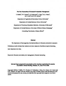
3. Policy simulations In this section, we present selected simulation results. Figure 2 shows the optimal dynamic path of the five state variables, together with exogenous forage production. They are calculated annually for 30 years without any restrictions imposed other than biophysical capacity constraints. Note that the dynamic simulation is performed by optimizing the dynamic model at each year, based on the information available to the producer in that year. The time series of forage production were generated by randomly drawing from the gamma distribution discussed earlier. (Note that bodyweight level (BW) is multiplied by ten in the figure for scaling purposes.) Given the relative prices and biological and forage limitations, the model predicts that it is not profitable to keep wethers. Indeed, wethers are usually kept for wool production, but with the depressed wool price, producers in Kazakhstan tend not to keep wethers. Since the sheep mature in about two years, keeping older wethers does not make sense for meat/fat type breeds. Ewe bodyweight fluctuates closely with forage production, but its volatility is softened by winter feeding. The most interesting result here is the producer’s response to the fluctuating forage production. The generated forage time-series exhibit a declining trend for the first 14 years, followed by years of higher average production with three peaks in years 15, 18,
17
and 23, and then years of very low forage production. In Figure 2, the EWE stock keeps increasing until year 14, but declines sharply in year 15.
With feed supplements
sufficiently available, the producer builds up his flock actively even if forage production is not very good. When a good year comes, he sells many of his sheep because animals are bigger and the price is higher. During the low forage production after year 25, the producer starts to build his flock again. Next, we considered the system where feed barley availability is limited. We repeated the SDP stage with barley limited to maximum of 0.3 kg per head per day (instead of the biological maximum of 0.8 kg that a sheep can eat in a day). This assumption of limited feeding per head, as opposed to a restriction on the total amount of barley available,3 may apply when feed supply or purchase takes place multiple times, but each time in a small amount. The flock dynamics with limited barley availability per head is simulated with the new set of Chebychev polynomial coefficients. In Figure 3, the EWE series from the two systems are contrasted. We notice that the two series move rather closely when forage production is good, but that in bad years the optimal strategy diverges significantly. The EWE series in the system with limited barley moves with the no restriction case until year 8. Year 9 is one of the worst years in terms of forage production. With the limited supplementary feeding, the shock of scarce forage during the grazing season cannot be repaired during winter, and rather than letting many sheep to die (mortality occurs in winter), the producer decides to sell even though the sheep price is low because of low sales bodyweight. After this period, the flock recovers as the forage production improves. Year 23 is a very good forage year, but two years later in
3
This case with total barley use for the entire flock in a year limited up to 20 ton was also simulated. The results were very similar to the case without any restriction, but the flock size was scaled down.
18
year 25 forage production is very low. In year 23, the producer receives high price due to high sales bodyweight, and many sheep is sold in both systems. In year 25, with adverse forage production, the optimal strategy diverges again. In the case of limited barley availability, the producer decides that it is not worthwhile to feed the small flock of weak animals and continue his operation. He gives up the enterprise for good. In contrast, with unlimited barley, flock size in year 25 increases slightly. Thus, the ability to feed sufficiently not only saves weak animals in bad forage years, but also works as insurance against potentially risky decisions, such as sales of large number of sheep in this case. One may argue that the behavior of the producer in the current model is rather extreme. Indeed, we assumed that the producer is risk neutral in the current specification. But we believe that sheep producers are risk averse in Kazakhstan, where the economy is still in transition and the government’s policies on livestock production are not clear. In future exercises, we plan to address issues of risk aversion.
We also plan to explore and evaluate the current government’s policies,
namely the pure breed subsidies and supports in veterinary services.
4. Discussion We applied the stochastic programming approach to an extensive livestock production problem. In the implementation, we followed the approach developed in Howitt et al. (2002), in which we first numerically approximated the value function, and then solved sequential optimization problems based on the approximated value function. The method allows us to handle multiple state and control variables, as well as modeling of complex biophysical relationships and stochasticity of the parameters, at a relatively
19
cheap computational cost. Moreover, unlike many conventional SDP implementations that use transition matrices, the feasible set for both state and control variables in the optimization in the simulation phase is continuous. Therefore, the models can achieve a much higher resolution, and researchers can have clearer vision and deeper insight about the problem. We applied the method to extensive sheep production in Kazakhstan. The results, though preliminary, suggest that this tool allows us to better model producers’ complex decision making when faced with dynamic, stochastic production problems involving numerous dimensions. The simulation exercises suggest that production of wool-type sheep is profitable when winter feeding is cheaply available. Such practices may have been possible with feed subsidies during the Soviet period, but are not consistent with the currently observed low-input low-cost production. The breeds developed during the Soviet period under the assumption of highly elastic feed supply may not be appropriate under the new system of market economy and extensive low-cost production. At the same time, we must be careful when interpreting the results and deriving policy conclusions. First, the simulation results are based on the assumption that the producer has expectations about the steady-state environment in which he operates and that his decision making is based on the expectations. In a situation where expectations are changing, such as in Kazakhstan in the last decade, the application of this model will require sequential updating.
Technically, we have to recalculate the Chebychev
polynomial coefficients before applying the simulation stage to the new environment. In addition, the biophysical relationships used in the current model are also an approximation of the complex reality, and the simulation results may be distorted due to
20
this simplification. We must always go back and check the results with data, more comprehensive biological simulation models, and specialists.
21
Figure 1. Sheep Management Calendar t
t+1
Month of Production Year A
M
J
J
A
S
O
N
D
J
F
M
A
M
Forage production (FPRODt)
Forage production (FPRODt+1)
Supplementary feeding (GHAYt, BARt)
Grazing (FORAGEt)
Lambing (βt) Æ LAFt, LAMt
Grazing (FORAGEt+1)
Lambing (βt+1) Æ LAFt+1, LAMt+1
Breeding Conception
Lactation, lamb mortality (δLAt)
Shearing (WLYt)
J
Lactation, lamb mortality (δLAt+1)
Mortality (δt)
Sales at sales bodyweight (SBWt)
State variables BWt YRFt YRMt EWEt WETt
BWt+1 YRFt+1 YRMt+1 EWEt+1 WETt+1 22
Shearing (WLYt+1)
Time
Figure 2. Simulation result: end-of-period states and forage production (No restriction on barley availability)
YRF/YRM/EWE/WET (head); BW (kg*10); FPROD (kg/ha/year)
1200
1000
800
600
400
200
0 1
2
3
4
5
6
7
8
9
10 11 12 13 14 15 16 17 18 19 20 21 22 23 24 25 26 27 28 29 30 Year
YRF
YRM
EWE
23
WET
BW*10
FPROD
Figure 3. Simulation result: end-of-period ewe stock and forage production (With and without restrictions on barley supplements) 1200
EWE (head); FPROD (kg/ha/year)
1000
800
600
400
200
0 1
2
3
4
5
6
7
8
9
10 11 12 13 14 15 16 17 18 19 20 21 22 23 24 25 26 27 28 29 30 Year EWE (no restriction)
EWE (limited barley)
24
FPROD
Table 1. Parameter Estimates for Biological Equations
α0 α1 α2 α3 α4 α5 α6 α7 α8 α9 α10 α11 α12 α13 α14 R2 n
(1)
(4)
(5)
(7)
(12)
(13)
FORAGEt
∆SBWt
∆BWt
βt
δt
WLYt
0.0687
-4.1262
-0.1017
1.1778
0.0244
1.7507
0.1153
0.0000
0.0655
20479873.2755
0.0305
0.0118
-0.0014
0.0218
0.0075
0.3823
-23.0065
2.0976
-0.0184
0.0028
0.0078
0.0000
0.0000
-0.00017
0.0022
-0.0109
-0.2939
0.000065
-0.00010
0.000016
0.0482
0.0000
-0.0061
0.00026
-0.1465
0.0000 0.00037 0.000028 0.0000 0.000069 0.8346 5267
0.7850 11389
0.8494 11389
0.9133 13867
0.8851 14762
Table 2. Price Parameters Used in the Current Model Average sheep price Wool price Grass hay price Barley price Shearing cost Herding cost
US$60.00 per head US$1.00 per kg US$0.70 per ton US$90.00 per ton US$0.15 per head US$1.00 per head per month
25
0.6459 14784
References: Frasier, W. Marshall, and George H. Pfeiffer. “Optimal Replacement and Management Policies for Beef Cows.” American Journal of Agricultural Economics 76(1994): 847-58. Howitt, Richard, Siwa Msangi, Arnaud Reynaud, and Keith Knapp. “Using Polynomial Approximations to Solve Stochastic Dynamic Programming Problems: or A “Betty Crocker” Approach to SDP.” Working paper, Department of Agricultural and Resource Economics, University of California, Davis, July 2002. Jarvis, Lovell S. “Cattle as Capital Goods and Ranchers as Portfolio Managers: An Application to the Argentine Cattle Sector.” Journal of Political Economy 82(1974): 489-520. Karp, Larry, and Arden Pope, III. “Range Management under Uncertainty.” American Journal of Agricultural Economics 66(1984): 437-46. Passmore, G., and C. Brown. “Analysis of Rangeland Degradation Using Stochastic Dynamic Programming.” Australian Journal of Agricultural Economics 35(1991): 131-57. Robinson, S., E. J. Milner-Gulland, and I. Alimaev. “Rangeland Degradation in Kazakhstan during the Soviet Era: Re-examining the Evidence.” Journal of Arid Environments 53(2003): 419-39. Standiford, Richard B., and Richard E. Howitt. “Solving Empirical Bioeconomic Models: A Rangeland Management Application.” American Journal of Agricultural Economics 74(1992): 421-33. Tozer, Peter R., and Ray G. Huffaker. “Dairy Deregulation and Low-input Dairy Production: A Bioeconomic Evaluation.” Journal of Agricultural and Resource Economics 24(1999): 155-72.