Modeling Seasonal Distribution and Spatial Range - Wyoming ...

ALCES VOL. 46, 2010

BAIGAS ET AL. – HABITAT MODELING IN SOUTHEAST WYOMING

MODELING SEASONAL DISTRIBUTION AND SPATIAL RANGE CAPACITY OF MOOSE IN SOUTHEASTERN WYOMING Phillip E. Baigas1, Richard A. Olson1, Ryan M. Nielson2, Scott N. Miller1, and Frederick G. Lindzey3 University of Wyoming, Department of Renewable Resources, 1000 E. University Ave., Laramie, WY 82071, USA; 2Western Ecosystems Technology, Inc. 2003 Central Ave., Cheyenne, WY 82001, USA; 3 17 Millbrook Rd. Laramie, WY 82070, USA. 1

ABSTRACT: Predictive maps of Shiras moose (Alces alces shirasi) habitat associations have not been created for most Wyoming populations. For the state’s most recently established population in the southeastern mountains, a literature-based winter habitat suitability index (HIS) model was developed and assessed with locations of 23 moose wearing global positioning system (GPS) radio-collars in 2005-2006. Overall, the winter HSI model was poorly predictive of habitat occupancy. The relationship between individual utilization distributions and landscape variables was modeled with resource selection functions (RSF) during winter and non-winter periods. In winter, moose generally responded in a similar fashion to distance variables to riparian shrub, to deciduous forest and forest edge, and slope and slope2. Due to snow pack differences, 2 separate models were created for each winter; thermal aspect (warm vs. cool slopes) rather than slope and slope2 was more predictive in the winter of deeper snow. The non-winter model demonstrated the nearly exclusive importance of riparian shrub habitat in close proximity to forest cover across a wide range of elevations. Non-winter moose locations were best explained by the total area of riparian shrub patches within a surrounding 1 km radius. Distance to forest edge had a considerably stronger influence on non-winter habitat use. The association with deciduous forest was still significant, although less than during winter; slope was also explanatory. The models were validated and a spatial algorithm was employed to estimate carrying capacity within the study area based on the predicted RSF habitat quality and size of winter home range.

ALCES VOL. 46: 89-112 (2010) Key words: Alces alces shirasi, capacity, global positioning system (GPS), habitat modeling, model validation, moose, resource selection function (RSF), Snowy Range, utilization distribution (UD), Wyoming.

Shiras moose (Alces alces shirasi) habitat in the Rocky Mountains of North America has been described by many authors. While moose are most commonly found in riparian shrub habitat types, other important habitats include mixed mountain shrub, aspen (Populus spp.), and conifer forest (Benson et al. 1987, WGFD 1990). Willow (Salix spp.) is considered the crucial forage of most moose in winter (Harry 1957, Houston 1968, Dorn 1970, Peek 1974) as well as the growing season (Zimmermann 2001, Dungan and Wright 2005). However, the spatial distribution of Wyoming’s Shiras moose relative to available habitat and for-

age resources is poorly documented for most populations, hence, seasonal range maps used by the Wyoming Game and Fish Department (WGFD) are undeveloped. The range of environmental situations exploited by moose during different seasons has only been defined recently for a single population in northwestern Wyoming (Becker 2008). Moose became established in the Snowy Range of the Medicine Bow Mountains in southeastern Wyoming following introductions in North Park, Colorado (approximately 50 km to the south) in the late 1970s (Duvall and Schoonveld 1988). The population has 89

HABITAT MODELING IN SOUTHEAST WYOMING – BAIGAS ET AL.

grown to a point that habitat condition is of concern and harvest has been liberalized. Of 38 moose hunting areas, the Snowy Range area is among those allowing highest opportunity with 45 permits (WGFD 2009). Harvest data and sightings suggest that the population continues to be very productive, whereas populations in western Wyoming are mostly in decline. Relationships among environmental variables and the distribution of wildlife are commonly described by spatially explicit models of habitat capability using geographic information systems (GIS). Species-habitat relationships and related maps are commonly used to develop expert opinion-based habitat suitability index (HSI) models. Allen et al. (1987) published one of the first HSI models for moose range in the Lake Superior region; subsequent models have been developed for several other regions (Romito et al. 1999, Koitzsch 2002, Snaith et al. 2002, Dussault et al. 2006). Advances in geospatial databases and remote animal observation technologies have compelled the development of more statistically reliable habitat modeling techniques. For example, resource selection functions (RSF) allow creation of maps that allow probabilistic predictions of habitat selection across large areas (Manly et al. 2002). Estimating Shiras moose populations in the Rocky Mountains is a management challenge. Although population surveys are generally reliable in areas where moose winter among extensive floodplains, their effectiveness may be limited by high cost or unfavorable weather conditions (Ward et al. 2000). However, population estimates are arguably necessary to develop management strategies and engage the public; likewise, carrying capacity estimates are desirable and useful to assess big game and domestic livestock range. Carrying capacity estimates require extensive information about vegetation dynamics and population demographics, and even with comprehensive data about forage

ALCES VOL. 46, 2010

biomass and nutritional quality, estimates differ by site, season, and even daily (Hanley and McKendrick 1983). Such variation makes an accurate carrying capacity estimate impossible in most cases, particularly where animals utilize multiple habitat types within variable habitats (McLeod 1997). It has been suggested that statistically robust RSF models can be combined with knowledge of a species’ behavioral ecology to estimate carrying capacity (Boyce and MacDonald 1999). A recent focus of many species-habitat studies is to relate habitat selection models (i.e., RSF maps) to various population metrics including home range (Boyce and Waller 2003, Apps et al. 2004, Mowat et al. 2004, Nielsen et al. 2005, Aldridge and Boyce 2007, Ciarniello et al. 2007; see Johnson and Seip 2008). Home range defines an accumulation of resources necessary for an animal’s survival and reproduction (Mitchell and Powell 2004) as determined by energetic requirements (McNab 1963), is considered economical (Powell 2000), and some minimum level of total habitat quality should be within a home range (Roloff and Haufler 1997, Mitchell and Powell 2004, 2007). Ecological and physiological factors are thought to influence home range size above a threshold level of habitat quality (McLoughlin and Ferguson 2000); home ranges are expected to contain approximately equal levels of total habitat quality assuming minimal variation in individual resource requirements. If habitat characteristics used to predict species distribution reflect those factors limiting survival and reproduction, then spatial calculations based on home range size and quality can estimate carrying capacity (Roloff and Haufler 1997). Moose density varies widely across their range (Maier et al. 2005) with individual variation in habitat use strategies (Osko et al. 2004, Dussault et al. 2005b). Resource requirements within a population are best compared during the critical winter period when forage is often limiting (Peterson and Allen 1974, WGFD 90

ALCES VOL. 46, 2010


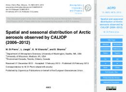
1990). We explored the total habitat quality of winter ranges as predicted by winter RSF models relative to winter range size. Our goal was to identify key habitat parameters of winter range for use in spatial calculations to predict carrying capacity of Shiras moose in southeastern Wyoming. STUDY AREA This study was conducted in the Snowy Range of the Medicine Bow Mountains of southeastern Wyoming. The study area is defined by the original boundary of Moose Hunt Unit 38, approximately 5,950 km2 (Fig. 1). Most moose range lies within the Medicine Bow National Forest (MBNF) that occupies approximately 35% of the study area. Another 15% of the study area was public land managed by the Bureau of Land Management, the State of Wyoming, and WGFD. Private lands dominating the surrounding Laramie Basin and North Platte River Valley accounted for nearly half the study area (2,890 km2). The climate is generally characterized by long, cold winters and short, dry summers. Most precipitation comes as snowfall in November-April, with accumulation varying greatly with elevation and exposure. Snow pack provides most of the available moisture during the short growing season (Knight 1994). Total annual precipitation typically ranges from 50-125 cm (USDA-NRCS 2007a), increasing with elevation due to snowfall accumulation. Much of the study area frequently experiences high velocity westerly winds that widely redistribute snowfall. Elevations range from 2,011 m above mean sea level along the North Platte River to 3,663 m atop Medicine Bow Peak. The greatest rise in elevation is in the central portion of the study area where the Snowy Range is formed by a steep face of uplifted granite. The remainder of the Medicine Bow Mountains is generally characterized by rolling, less dramatic topography. However, many creeks cut steep ravines or canyons through

Fig. 1. Location of study area in Moose Hunt Area 38 in southeast Wyoming, USA.

the foothills as they descend from montane elevations on all sides. Over 50% of the forest area is comprised of lodgepole pine (Pinus contorta) at various densities. These stands typically have a sparse understory of scattered buffaloberry (Sheperdia canadensis) and common juniper (Juniperus communis), with heartleaf arnica (Arnica cordifolia) as the primary herbaceous species. An Engelmann spruce (Picea engelmanii)–subalpine fir (Abies lasiocarpa) association typically occurs at higher elevations with an understory primarily of mosses and dwarf huckleberry (Vaccinium scoparium); Englemann spruce and subalpine fir also grow within sheltered ravines and along stream corridors at lower elevations. Interspersed within the coniferous forest and commonly in drainage bottoms are clones of quaking aspen (P. tremuloides) at elevations up to 2,900 m. Common aspen associates are serviceberry (Amelanchier alnifolia), snowberry (Symphoricarpos spp.), gooseberry/currant (Ribes spp.), redosier dogwood (Cornus sericea), Woods rose (Rosa woodsii), and Scouler willow (Salix scouleriana). Willow communities occur in riparian areas, varying in species composition by elevation. In general order of greatest abundance, willow species included planeleaf (Salix planifolia), Booth (S. boothii), Wolf (S. wolfii), Drummond (S. drummondiana), Geyer (S. 91


geyeriana), whiplash (S. lasiandra), mountain (S. monticola), strapleaf (S. eriocephala var. ligulifolia), Bebb (S. bebbiana), and yellow (S. eriocephala var. watsonii). There are approximately 53 km2 of willow communities within the study area, accounting for 1.3% of the MBNF. Bog birch (Betula glandulosa) is widely distributed in association with shorter willow species on moderately sloping stream gradients. At lower elevations, cottonwood species such as balsam poplar (Populus balsamifera) and narrowleaf cottonwood (P. angustifolia) create forest corridors along stream margins with taller willows (Drummond, Bebb, whiplash, and yellow) in the adjacent floodplain. Irrigated hay meadows are adjacent to most major streams below the forest. Approximately 20% of the MBNF is not forested occurring as alpine meadows, natural openings or parks, regenerating clearcuts, riparian meadows, or dry slopes. Mountain big sagebrush (Artemisia tridentata ssp. vaseyana) and antelope bitterbrush (Purshia tridentata) dominate a mixed grass-shrub community at foothill elevations with southern exposure. Associated thickets of true mountain mahogany (Cercocarpus montanus), serviceberry, and snowbrush ceanothus (Ceanothus velutinus) are widely scattered. Traditional land uses in the forested portion of the study area include timber extraction, mining, and livestock grazing, although these activities have declined. Consumptive and non-consumptive recreational use is increasingly important due to the proximity of human population centers in southeastern Wyoming and north-central Colorado. Cattle ranching operations dominate non-forested private lands.

ALCES VOL. 46, 2010

CO2-injection powered rifle (Dan-inject North America, Fort Collins, CO) was used to fire 13 mm, 1.5 mL darts equipped with 32 mm barbed needles (Pneu-dart, Williamsport, PA) containing a dose of 10 mg thiafentanil (Kreeger et al. 2005). Immobilized moose were blindfolded and blood, hair, and swab samples of fecal and ear material were collected. The antibiotic oxytetracycline was administered to protect against dart wound infection, and Imovec was injected for endoand ectoparasite control. Thiafentanil was antagonized with 300 mg naltrexone. Adult females were captured preferentially over males at a 3:1 ratio (Kreeger et al. 2005) to document female productivity, yet provide comparison of habitat use between sexes. Captures were performed in accordance with the University of Wyoming Institutional Animal Care and Use Committee protocols. Each moose was fitted with a store-onboard Global Positioning System (GPS) collar (Model TGW 3700, Telonics, Mesa, AZ) programmed to collect locations every 1.5 h. A CR-2a release mechanism allowed for pre-programmed collar release. Sixteen collars were deployed December 2004; 8 were programmed to release in June 2005 and 8 in August 2006. The 8 collars collected in June 2005 and 2 collars from bulls harvested in October 2005 were redeployed in December 2005 and programmed to release in June 2006. Two bulls captured in December 2005 did not survive and 1 cow captured in December 2005 was an unintentional recapture. In total, 23 moose were studied; 16 were 1-winter animals (6 M, 10 F) and 7 were 2-winter animals (1 M, 6 F). GPS locations and other spatial datasets were projected in NAD 83, UTM Zone 13 and managed with ArcGIS 9.2 (Environmental Systems Research Inc., Redlands, CA 2007).

METHODS Moose Captures Moose were tranquilized from a helicopter (n = 23) or the ground (n = 3) in December 2004 (5 M, 11 F) and 2005 (4 M, 6 F). A

Vegetation and Spatial Data A classified 30-m Landsat ETM+ image of the study area was obtained (Driese and 92

ALCES VOL. 46, 2010


Nibbelink 2003) and used as the foundation for a preliminary HSI model. The Resource Information System (RIS; USFS 1995), a forest stand polygon database maintained by the MBNF, was used to develop observationbased RSF models. The RIS layer provided an effective basis for calculating a distance to forest edge variable. However, inconsistent results from queries of this database to identify forest attributes believed important to moose (e.g., species mix, percent cover, stand age, stand density) made it necessary to generalize forested polygons into 3 forest types: coniferous, deciduous, and mixed forest. Polygons attributed as containing >95% conifer forest were grouped together, regardless of species composition. RIS polygons with >75% aspen were identified as deciduous forest. Conifer stands with >5% aspen were classified as mixed forest; mixed forest polygons were often pure coniferous stands containing small patches of deciduous forest. Such cases were isolated by visual review of 1-m color infrared (CIR) orthophotography (2002) and the deciduous patches were heads-up digitized. The RIS layer did not cover the entire study area, so additional editing was required to define the distribution of important cover types. Landsat image pixels beyond the extent of the RIS dataset were classified as deciduous forest and converted to polygons that were modified where necessary to better reflect aspen stand boundaries; polygons were deleted where misclassification occurred. Lastly, deciduous forest stands not identified by either vegetation layer were heads-up digitized using the CIR imagery. Likewise, because neither dataset accurately delineated riparian cover types, all riparian shrub communities discernable on the CIR photos were digitized across the study area. The National Wetland Inventory (NWI; USFWS 2007) dataset was used to identify riparian areas and polygons were modified to the boundaries of riparian shrub communities. New polygons were created around riparian shrub communities in locations not

identified by the NWI. Euclidean distances to deciduous forest and riparian shrub polygons were calculated as variables. We calculated distances to snowmobile trails and maintained gravel roads. Distance to “high resolution” flowlines of the National Hydrography Dataset, derived from 1:24,000 topographic maps (USGS 2000), was calculated as a variable. For each distance variable, a centered 2nd order polynomial term was calculated for consideration in statistical model building (Kutner et al. 2003). Additional predictor variables were compiled to explore topographic influences on habitat use. A 30-m digital elevation model (DEM; USGS 1999) was obtained and the Spatial Analyst extension (Environmental Systems Research Inc., Redlands, CA 2007) was used to calculate slope (degrees) and aspect. Grid cells with slope >4º were assigned to 1 of 8 categories (N, NE, E, SE, S, SW, W, or NW). Areas with slight slopes (≤4º) were considered flat and assigned to a reference category. A thermal aspect was created to differentiate between warm and cool slopes. Slopes ≥4º facing NW, N, NE, or E were assigned a “cool” value of 0, and south- or west-facing slopes were assigned a “warm” value of 1. To account for potential interaction between these variables, a site severity index (SSI; Nielsen and Haney 1998 in Boyce et al. 2003) was calculated from slope (%) and aspect (A, in degrees) as follows:  slope SSI = sin(Α + 225)*    45 

(1)

Values ranged from -3.59 on steep northeast slopes to 4.23 on steep southwest slopes, with moderate slopes having values ±0. Variables were computed to describe cover type arrangement and the amount of forest edge surrounding a given point on the landscape within 2 distances, since habitat selection occurs at different scales (Johnson 1980). Eight variables were derived using the moving window algorithm (Focal Sum) of 93


ALCES VOL. 46, 2010

elevations were set at 0. Optimal slopes were those ≤10º and suitability decreased linearly with increasing slope to SI2 = 0 at slope ≥60º. Similarly, locations within 120 m of a riparian shrub polygon had SI3 = 1 and decreased linearly with increasing distance to SI3 = 0 at distances ≥360 m. Foraging habitat capability was determined based on the assumed vegetation quality and production within the Landsat cover class. Riparian forest, mesic shrubland, and mixed mountain shrubland were assigned optimal suitability; deciduous forest, mixed forest, and mixed mountain shrub were assigned SI4 = 0.5. Cover classes deemed least suitable for foraging (SI4 = 0) included grassland and conifer forest, among others (Table 1). Because larger willow patches may accumulate more snow and provide less protective cover for moose, the extent of contiguous riparian shrub pixels was calculated using the moving window algorithm (150 x 150 m) of the Spatial Analyst extension. Optimal riparian shrub patches (SI5 = 1) were defined

the Spatial Analyst extension (Environmental Systems Research Inc., Redlands, CA 2007). The approximate mean distance between consecutive locations (80 m) and the mean cumulative 24-h distances among locations (1 km) defined the radius of 2 circular windows that were centered on each raster cell. Within each buffer distance the area of intersecting coniferous forest, deciduous forest, and riparian shrub was summed; the total distance of forest edge within these 2 buffers was also calculated. Winter HSI Model Creation A knowledge-based HSI model was developed with 5 variables identified as important to Shiras moose in western North America: elevation (SI1), slope (SI2), distance to willow (SI3), food availability (SI4), and willow patch size (SI5) (Table 1). Locations at elevation of 2,439-2,896 m were assigned an optimum suitability index value (SI1 = 1), lower elevations were assigned SI1 = 0.5, and higher

Table 1. Description of 5 variables considered important to Shiras moose in western North America that were used to develop a preliminary habitat suitability index (HSI) model in southeastern Wyoming. Variable SI1

SI2

SI3

SI4

SI5

Elevation

Slope

Distance to willow

Food availability

Criteria

HIS

> 2,896 m

0

< 2,439 m

0.5

Reference Personal Observations; and

≤ 2896 & ≥ 2439 m

1

WGFD Annual Reports

≥ 60º

0

Langley 1993;

> 10º & < 60º

0–1

≤ 10º

1

> 360 m

0

≥ 120 & ≤ 360 m

0–1

Rudd and Irwin 1985; and Van Dyke 1995 Kufeld and Bowden 1996; and

< 120 m

1

Halko et al. 2001

Grassland, sagebrush shrubland, rock, etc.

0

Peek 1974;

0.5

Harry 1957;

Deciduous forest, mixed forests, mixed mountain shrubland Riparian forest, mesic shrubland, riparian shrubland

> 2 ha Willow patch ≤ 2 ha & ≥ 1.75 ha size < 1.75 ha

1

Houston 1968

0 0.5 1

94

Personal Observations

ALCES VOL. 46, 2010


sampling point was also intersected with the underlying grid value of each potential variable layer. Predictor variables were screened for collinearity and if correlations were large (r >0.6), they were not included in the same model. RSF models were developed for both winter and non-winter using locations from both years. Separate winter 2005 and winter 2006 RSF models were also created because cover type selection and diet composition differed between years (Baigas 2008). A general linear model (GLM; Eq. 3) was fit for each individual moose, assuming a zero-inflated negative binomial (NB) distribution in order to allow for overdispersion (i.e., clustering):

as those >0 ha and 2 ha were assigned SI5 = 0. Variables were stored in GRID format and a linear combination was spatially projected across the study area as:

(

)

1/5

HSI = SI1 * SI 2 * SI 3 * SI 4 *SI 5

(2)

This HSI model was evaluated with the winter locations of moose. RSF Model Estimation The definition of winter was determined by reviewing the contraction and expansion of moose range, as energy and forage availability are constrained by snow depth. A 95% kernel density estimate polygon was created from locations of each moose in 2-week time steps using Hawth’s Tools (Beyer 2006). The bi-weekly interval in which moose movement became dramatically limited was defined as the start of winter, lasting until range expansion was observed in spring. The rest of the year was considered a single non-winter period. Resource selection functions (Manly et al. 2002) were calculated following methods described by Marzluff et al. (2004), Millspaugh et al. (2006), and Sawyer et al. (2006, 2007). Individual animals defined the sample unit, rather than GPS point locations, which allows for the identification of individual differences in habitat selection (Osko et al. 2004) and avoids concerns about spatial autocorrelation and pseudoreplication (Sawyer et al. 2007). The domain of analysis was defined by a 100% minimum convex polygon around all moose locations, as recommended by McClean et al. (1998). Sampling points (n = 68,387) were created within this area from the centroids of a 125-m raster grid. The number of locations within each grid cell was tallied for each moose separately as a surrogate utilization distribution (UD; Marzluff et al. 2004), and transferred as an attribute of each sampling point using Hawth’s Tools (Beyer 2006). Each

ln[E (ri )]= ln(total )+ β 0 + β1 x1 + β 2 x 2 + ... + β p x p

(3)

where ri is the expected number of point locations for that moose within grid cell i, total is an offset term equal to the total number of GPS points collected from that individual, and predictor variables x1 ... xp have coefficients β1 ... βp (Millspaugh et al. 2006). Using a forward stepwise modeling approach, variable entry was determined by considering the collective direction and strength of individual moose responses (Sawyer et al. 2006). After running the NB GLM model for each moose, coefficients of each variable were assumed to be a random sample taken from a standard normal distribution. Using the mean and standard error, a t-statistic was calculated to test the likelihood of the coefficient’s deviation from normality. Variable entry was permitted at P ≤0.15 (Sawyer et al. 2006). For significant variables, coefficients were averaged among all moose to create population-level RSF models. After GLM coefficients were estimated for each RSF model, a log-linear model was used to calculate and spatially project the probability of use (w) for each 30 x 30 m raster cell. Coefficients (β1) were multiplied by each cell (xi) in the respective raster of predictor 95


variables x1 … xp as: w(x ) = exp(β 0 + β1 x1 + ... + β p x p )

separate locations among higher predictive classes and increased the sensitivity of the rank correlation. A good predictive model is defined as having high correlation (rs >0.90; Boyce et al. 2002) since an increasing number of animal locations fall within higher model classes. An overall measure of model fit was assessed by averaging the 5 rs values. One-winter RSF models were evaluated with the independent sample of moose from the other winter, excluding 7 moose collared both winters. Similar to 2-winter models, 1-winter RSF maps were classified by vingtiles and the number of locations within each class was tallied. Spearman rank correlations were calculated between the numeric RSF model classes and the counts of locations. The lower classes containing no locations were assumed to be unsuitable habitat. Because the exponential model can be an incorrect combination of estimated regression parameters and RSF models may not necessarily measure the absolute probability of use (Keating and Cherry 2004), further evaluation of 1-winter RSF maps was performed to determine if map predictions were indeed proportional to the likelihood of use. Within the portion of the study area identified as suitable moose habitat (occupied 2-winter RSF map vingtiles), the relative probability of use values (ŵ) of 1-winter RSF maps were reclassified into 10 equal-interval classes having values 0-1 at intervals of 0.1. The expected utilization value, U(xi), was then calculated as:

(4)

For easier visualization and comparison, the resulting raster values were scaled from 0-1 with a linear stretch with the following equation:   w( x) − wmin   w =   wmax − wmin 

ALCES VOL. 46, 2010

(5)

where wmin and wmax represent the smallest and largest RSF values, respectively (Johnson et al. 2004). Relative probability of use values (ŵ) were classified using the common approach of identifying quartile breakpoints. The 25th, 50th, 75th, and 100th percentiles were assigned to low, medium-low, medium-high, or high habitat value classes, respectively. Alternatively, a map of continuous ŵ values was maintained to present finer distinctions among RSF values. RSF Model Validation The winter and non-winter RSF models developed from locations of both years combined were evaluated using a 5-fold cross validation method (Boyce et al. 2002, Hirzel et al. 2006). The 23 moose were randomly partitioned into 5 groups (3 groups of 5 and 2 groups of 4). A RSF model was developed (Eq. 3) from moose within 4 groups (training set) and intersected with locations of moose in the withheld group (test set). This calibration and test procedure was performed 5 times, once for each training and test set combination. Estimated RSF models were projected to 30-m rasters (Eq. 4) that were classified into 20 equal area classes (vingtiles) occupying approximately 297 km2. For each individual moose in the test group, a Spearman rank correlation coefficient (rs) was calculated between the 20 model classes (i.e., 1, 2, 3, . . . 20) and the number of intersecting locations. The use of 20 bins, twice what Hirzel et al. (2006) recommended, was necessary to adequately

)= A(xi )* w(xi ) U (xi ∑ w(xi )* A(xi )

(6)

i

where A(xi) is the area and w(xi) is the RSF midpoint value of the ith class (i.e., 0.05, 0.15, 0.25, . . . 0.95; Boyce and McDonald 1999). The resulting U(xi) values describe the relative proportion of locations expected to occur within each of the 10 equal-interval classes, adjusted by area. The observed proportion of locations (Ni) from the other winter was calculated by dividing the frequency of 96

ALCES VOL. 46, 2010


points within the ith class by the total number of points. A simple linear regression model of Ni vs. Ui was fit to assess the relationship between observed and expected observation frequencies. A RSF model that is relatively proportional to the probability of use has a high R2 and slope not significantly different from 1 (Johnson et al. 2006). Statistical analyses were performed in the open-source programming application R, version 2.4.0 (R Foundation for Statistical Computing 2006). RSF modeling was performed using the “glm.nb” routine in the “MASS” library.

winter range. This number is equivalent to an arbitrary habitat units (HU) measurement, where 1 HU equals 1 ha at maximum resource potential (ŵ = 1) (Plume and Roloff 2005). Accordingly, 1 HU can be achieved with 100 cells having ŵ = 1, 200 cells having ŵ = 0.5, or 400 cells having ŵ = 0.25, and so forth. Home range size was plotted against its HU value to evaluate whether an RSF-based spatial calculation was appropriate for making capacity approximations. A lack of correlation between the 2 values would tend to provide support to the approach. The HomeGrower application developed by Plume and Roloff (2005) was used to estimate the number of moose home ranges that the study area could conceivably support. Its algorithm places a large number of random seed points (e.g., > 20,000) on the habitat quality map (i.e., RSF) and “grows” a home range outward until the target HU with a defined minimum threshold is accumulated. A successful home range occurs when the total RSF value meets or exceeds the HU target value before a defined maximum home range size is reached. Iterations of the procedure are run and successes are tallied until the grid is filled to capacity with hypothetical home ranges. A range of potential capacity approximations was computed by adjusting the target habitat quality parameter based on the mean, 25% quartile, and 75% quartile of HU values. These same summary statistics of winter home range size, including the maximum, were used to define the maximum allowable home range size.

Range Capacity Approximation Spatial calculations based on predicted winter RSF values and observed home range sizes (Roloff and Haufler 1997, 2002) were performed to provide a rough approximation of potential moose range capacity. Winter home ranges were delineated using the 95% adaptive local convex hull (a-LoCoH) method with the Getz and Wilmers (2004) ArcGIS toolbox. This algorithm connects each GPS point with a convex polygon to all neighboring points “within a radius, a, such that the distances of all points within the radius to the reference point sum to a value ≤ to a” (Getz et al. 2007). The union boundary of these polygons is taken to represent the home range boundary. A winter a-LoCoH home range was delineated for each moose with multiple a, and the appropriate value was determined when the estimated range size increased towards asymptote. The performance of each home range polygon was also visually reviewed with respect to the spatial distribution of locations. The 1-winter RSF model validated as best predictive of habitat use was used to explore how winter range size related to predicted home range quality. That model was applied to a 10 x 10 m raster with Eqs. 4 and 5. An overall home range “quality” was calculated by adding the relative probability of use values (ŵ) of raster cell within each moose a-LoCoH

RESULTS

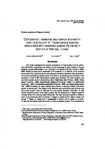
Habitat Models Winter HSI model -- A winter HSI model based on classified Landsat satellite imagery indicated that the best moose habitat occurred alongside streams at low elevations below the forest boundary (Fig. 2). These extensive floodplain willow complexes were among the most accurately predicted areas of highly suitable winter habitat. In addition, 97


moose that wintered within riparian shrub or aspen communities were mostly found within higher HSI prediction regions. However, the HSI model was poorly predictive of all winter locations. Pooled observations did not occur at increasing frequency within cells having higher HSI value (rs = 0.15), and approximately 50% of locations were in areas with HSI ≤0.5 (Fig. 2). Several moose occupied conifer forest or upland shrub cover types for a substantial part of winter, habitats classified as unsuitable winter range based on the input land cover parameters. Also, the HSI map produced questionable predictions of high suitability next to streams surrounded by rangelands at lower elevations. In fact,

ALCES VOL. 46, 2010

moose are rarely documented to occupy the 2 largest concentrations of predicted high quality winter habitat. Two-winter RSF model -- Movement of all moose became substantially limited the first week of January until mid-April; winter was thus defined as 1 January-15 April. A population-level winter RSF was first created from 48,992 locations obtained from 23 individuals during both winters; there were 1,656-1,665 locations/moose each winter. Moose responded similarly to 4 predictor variables (Table 2). Distance to forest edge explained the most variance of habitat use, followed by distance to deciduous forest and distance to riparian shrub; slope and slope2 were also significant variables. The model was applied to predict the probability of moose occurrence with Eq. 4 as:  − 10.329 − 0.0024( DistToRipShrub) − 0.0035( DistToDecidForest) −   w(x ) = exp 2   0.0039( DistToForestEdge) + 0.0782(Slope) − 0.0042(Slope ) 

Cross validation of this model indicated that it performed well ranking the value of winter habitat. Locations of moose in 5 cross-validation sets occurred with increasing frequency among bins of higher RSF values, producing Spearman rank correlations of 0.972, 0.919, 0.962, 0.866, and 0.925 (rs = 0.93). There were no moose observations in the lower 8 of 20 classes for any cross-validated model; therefore, approximately 40% of the study area could essentially be considered unsuitable winter habitat. If those unoccupied lower bins were ignored, 3 of 5 cross validation sets had rs = 1. One-winter RSF models -- Snow depth in 2005 averaged 87% of normal, ranging 8290% at 4 SNOTEL sites distributed across the mountain range. In 2006, mean depth at these sites was 126% of normal, ranging 115-134% (USDA-NRCS 2007b). To account for this annual difference, separate RSF models were estimated for each winter using 26,607 locations obtained from 16 moose in 2005, and 22,385 points from 14 moose in 2006.

Fig. 2. Map of a preliminary winter habitat suitability index (HSI) model based on the influence of elevation, slope, distance to willow, food availability, and willow patch size in southeastern Wyoming. This HSI model was validated with GPS collar points collected on a sample of moose during winter 2005 (n = 7) and winter 2006 (n = 9). 98

ALCES VOL. 46, 2010


Table 2. Mean negative binomial regression coefficients (b), standard errors (SE), and significance level (P) from 4 seasonal population-level resource selection function (RSF) models created to predict moose distribution in the Snowy Range of the Medicine Bow Mountains in southeast Wyoming, December 2004 – August 2006. Models were applied to predict the probability of occurrence with the equation, w(x) = exp(b0 + b1x1 + … + bpxp). Non-significant variables are identified as “ns”. All Winter

Intercept

b

SE

Winter 2005 P

b

Winter 2006

SE

P

b

SE

Nonwinter P

b

SE

P

0.2652

2,800 m within the forest foraging on 1.5-2 m willow, underscoring the importance of high biomass, tall willow complexes during the growing season. Interestingly, in winter 2006 with deeper snow she occupied predominately forest habitat between her 2005 seasonal ranges. Moose were close to forest edges at all times, more so than deciduous forest or riparian shrub communities. This association with forest edge could lead to the conclusion that fragmentation in the MBNF has benefited moose since a preference for edge habitat is widely reported across most of the boreal forest (Mastenbrook and Cumming 1989, Thompson and Stewart 1998), northwest Montana (Costain 1989, Matchett 1985), southeastern British Columbia (Poole and Stuart-Smith 2006), and Washington (Base et al. 2006).

ALCES VOL. 46, 2010

However, clearcuts with little or no browse regeneration are not utilized (Matchett 1985) and it is uncommon for site conditions in the southern Rocky Mountains to favor abundant browse production following harvest. Habitat use during winter was rarely near edges of timber harvests, as only 1 bull and 2 cows occupied clearcuts and only 1-2.5% of time; data from Colorado are similar (Kufeld and Bowden 1996). The preferred winter ecotone provided by edge was that between mature forest cover and upland or riparian shrub communities. However, it does appear that some moose were attracted to clearcuts >15 years old in August-October, particularly those adjacent to riparian areas with the requisite timber buffer (>100 m; USFS-MBNF 2004). The influence of solar radiation on use of south- and west-facing slopes has been previously reported (Langley 1993, Halko et al. 2001). The effect was greater during the year with less snow pack and presumably reflects higher availability of low-growing mountain shrub communities. However, while the significance of the thermal aspect differed between years (2005: P = 0.067, 2006: P = 0.163), the difference in pattern of use between aspects was less apparent. All moose used warm (south- or west-facing) aspects >50% of time in winter 2006, but 3 moose occupied cool (north- or east-facing) aspects more in winter 2005. The significance of thermal aspect in winter 2005 was probably due to 5 moose occupying warm aspects >75% of time, whereas only 1 moose made such exclusive use of warm slopes in winter 2006. Although the 2005 winter RSF model that included thermal aspect was less predictive than models with slope and slope2, the influence of solar insolation on snow depth and vegetation certainly influences moose distribution in the Snowy Range. Moose generally used slopes up to 20º during winter; use declined with increasing frequency on steeper slopes. The influence of slope was less consistent during winter

104

ALCES VOL. 46, 2010


2005 and was not included in the RSF model. That winter 7 of 16 moose (44%) used slopes between 0-5º most, and others occupied 5-10º slopes. In 2006, 11 of 14 moose (79%) were found most often on 5-10º slopes. The mean slope occupied by moose was 7.1º in 2005 and 9.3º in 2006; fewer observations were in flat areas (i.e., drainage bottoms) in 2006. The quadratic term of slope in the 2005 RSF had the effect of increasing suitability values to a maximum about 13º; suitability declined to 0 at approximately 40º. Underneath this curve all locations with slope 0.5. Lower slopes were occupied most frequently in non-winter because stream corridors were the preferred habitat, producing a model with highest suitability values in riparian areas. A difficulty with species distribution modeling is that models based on a single population or landscape may not necessarily translate well to other situations (Boyce and Waller 2003, Apps et al. 2004), particularly if habitat preferences are not fixed in moose (Osko et al. 2004). The application of this model across Shiras moose range would be complicated by local resource availability (Mysterud and Ims 1998), land management activities that produce habitat variation, as well as competition, weather, predation, and harvest (Peek 1998). These processes may influence distribution at different scales (Dussault et al 2005b, Dussault et al. 2006) leading to locally poor performance of a large-scale model. Accounting for such parameters should improve model accuracy and enhance the applicability of a model. The habitat quality values predicted by RSF models were assumed to correspond to the energetic efficiency of different habitat situations since they result from occupancy patterns of many individual moose. However, Saether and Andersen (1990) demonstrated that when moose are not able to select patches of highest quality, they modify their behavior to adapt to local conditions. The intensity of

use (i.e., UD) may only describe the relative habitat value of different sites (North and Reynolds 1996), which could explain the wide variation observed in predicted home range quality. Other factors contributing to the observed 4-fold variation in home range size probably include maternal influences, sex, age, body size, health status, and a variety of unmeasured environmental influences. Nonetheless, the total predicted RSF values within winter ranges did not tend to increase with home range size; larger ranges incorporated more area of “low quality” resources. Dussault et al. (2005a) also found a negative relationship between food availability and a wide range of moose home range sizes during winter, and this relationship has also been reported for several mammalian species (Litvaitis et al. 1986, Ims 1987, Jones 1990, Tufto et al. 1996, McLoughlin and Ferguson 2000, Mitchell and Powell 2007). The spatial approach to carrying capacity produced variable estimates, but were as accurate as those of a forage-based model that calculated willow production in North Park, Colorado (Kufeld and Steinert 1990) that had ~15% more riparian shrub habitat than our study area. Carrying capacity was estimated at ~1,800 animals (>29 moose per km2), an obvious overestimation indicating that moose are not limited by availability of willow browse, and the difficulty of estimating carrying capacity from browse availability and consumption data. Because of variation in plant and animal nutrition (Hanley and McKendrick 1983), estimates of ungulate carrying capacity based on forage production and a nutritionally optimal diet are often tenuous (Hanley and Rogers 1989). MANAGEMENT IMPLICATIONS Moose are difficult to manage in Wyoming due to their solitary nature, low density, and preference for forest habitat. Our habitat models are useful to identify core areas critical for survival of moose in the southern Rocky

105


Mountains. Such locations include montane riparian willow galleries surrounded by forest, the bottoms of foothill drainages as they exit forested cover, the steep south- and west-facing hillsides above those drainages, aspen stands encroached by subalpine fir, and floodplain willow communities. This information should be useful to improve the efficiency of population sampling and to identify critical habitats for monitoring. Although the empirical RSF models may be statistically objective in their explanation of habitat associations, a certain degree of subjectivity is necessary to apply them in other areas. Habitat models by nature cannot include every relevant parameter, and population density and habitat use are not always related to one defined set of predictor variables. Therefore, the RSF models described here may be difficult to apply directly to other areas, especially where such resolved vegetation data layers are not available. However, the relationships among cover, riparian shrub, and deciduous forest are probably similar for many other Rocky Mountain moose populations. There exist at least as many “carrying capacities” as there are management objectives (Heady 1975). A population biologist seeks to reach a balance where the public and landowners are satisfied with animal numbers, while important habitats are sustained for biodiversity. The moose population in the Snowy Range has experienced an irruptive growth phase in the past 20 years, and arguably, will be regulated increasingly by nutritional constraints from competition and decline in forage resources. Although body condition and reproductive health of animals handled in this study do not indicate such conditions exist currently, high use of preferred browse exists in the study area. Poor range condition has often been implicated as the cause of population declines, and a fine-scale, habitatbased approach has long been recommended to manage moose populations (Timmermann and Buss 1998). A conservative management

ALCES VOL. 46, 2010

strategy would be to assume that moose have reached capacity in the Snowy Range, and the population should be maintained at a sustainable level relative to key habitats identified in this study. ACKNOWLEDGEMENTS Eric Wald should be recognized for initiating this project, establishing research objectives, and securing a great deal of funding. We thank Bob Lanka and the efforts of many other WGFD personnel for their assistance with moose captures and other support services. John Haufler of the Ecosystem Management Research Institute graciously provided the use of the Homegrower application. WGFD and the Department of Renewable Resources, University of Wyoming provided funding. Additional support was provided by the Wyoming Governor’s Big Game License Coalition administered by the Wildlife Heritage Foundation of Wyoming. Bowhunters of Wyoming also provided financial assistance. REFERENCES Allen, A. W., P. A. Jordan, and J. W. Terrell. 1987. Habitat Suitability Index Models: Moose, Lake Superior Region. U.S. Fish and Wildlife Service Biological Report 82 (10.155), Fort Collins, Colorado, USA. Aldridge, C. L., and M. S. Boyce. 2007. Linking occurrence and fitness to persistence: habitat-based approach for endangered greater sage-grouse. Ecological Applications 17: 508-526. Apps, C. D., B. N. McLellan, J. G. Woods, and M. F. Proctor. 2004. Estimating grizzly bear distribution and abundance relative to habitat and human influence. Journal of Wildlife Management 68: 138-152. Arlt, D. 2007. Habitat selection: demography and individual decisions. Ph. D. Dissertation, Swedish University of Agricultural Sciences, Uppsala, Sweden. Baigas, P. B. 2008. Winter habitat selection, winter diet, and seasonal distribution

106

ALCES VOL. 46, 2010


mapping of Shiras moose (Alces alces shirasi) in southeastern Wyoming. M.S. Thesis, University of Wyoming, Laramie, Wyoming, USA. Base, D. L., S. Zender, and D. Martorello. 2006. History, status, and hunter harvest of moose in Washington state. Alces 42: 111-114. Becker, S. A. 2008. Resource selection and population dynamics of Shiras moose (Alces alces shirasi) in northwest Wyoming. M.S. Thesis, University of Wyoming, Laramie, Wyoming, USA. Benson, S., J. Emmerich, and R. Olson. 1987. Lander Moose Herd Unit Winter Range Study. Wyoming Game and Fish Department, Cheyenne, Wyoming, USA. Beyer, H. L. 2006. Hawth’s analysis tools: an extension for ArcGIS. < http://spatialecology.com/> (accessed July 2009). Boyce, M. S., and L. L. McDonald. 1999. Relating populations to habitat using resource selection functions. Trends in Ecology and Evolution 14: 268-272. _______, J. S. Mao, E. H. Merrill, D. Fortin, M. G. Turner, J. Fryxell, and P. Turchin. 2003. Scale and heterogeneity in habitat selection by elk in Yellowstone National Park. Ecoscience 10: 421-431. _______, P. R. Vernier, S. E. Nielsen, and F. K. A. Schmiegelow. 2002. Evaluating resource selection functions. Ecology Modeling 157: 281-300. _______, and J. S. Waller. 2003. Grizzly bears for the Bitterroot: predicting potential abundance and distribution. Wildlife Society Bulletin 31: 670-683. Ciarniello, L. M., M. S. Boyce, D. C. Heard, and D. E. Seip. 2007. Components of grizzly bear habitat selection: density, habitats, roads, and mortality risk. Journal of Wildlife Management 71: 1446-1457. Corsi, F., J. De Leeuw, and A. K. Skidmore. 2000. Modeling species distribution with GIS. Pages 389-434 in L. Boitani and T. K. Fuller, editors. Research Techniques

in Animal Ecology: Controversies and Consequences. Columbia University Press, New York, New York, USA. Costain, W. B. 1989. Habitat use patterns and population trends among Shiras moose in a heavily logged region of northwest Montana. M.S. Thesis, University of Montana, Missoula, Montana, USA. Courtois, R., and A. Beaumont. 2002. A preliminary assessment on the influence of habitat composition and structure on moose density in clear-cuts of northwestern Québec. Alces 38: 167-176. Dorn, R. D. 1970. Moose and cattle food habits in southwest Montana. Journal of Wildlife Management 34: 559-564. Driese, K. L., and N. P. Nibbelink. 2003. SE Wyoming Cumulative Impacts Project: Mapping Land Cover and Land Cover Change in SE Wyoming. Wyoming Geographic Information Science Center, University of Wyoming, Laramie, Wyoming, USA. Dungan, J. D., and R. G. Wright. 2005. Summer diet composition of moose in Rocky Mountain National Park, Colorado. Alces 41: 139-146. Dussault, C., R. Courtois, J. Huot, and J.-P. Ouellet. 2001. The use of forest maps for the description of wildlife habitats: limits and recommendations. Canadian Journal of Forestry Research 31: 1227-1234. _____, _____, J.-P. Ouellet, and I. Girard. 2005a. Space use of moose in relation to food availability. Canadian Journal of Zoology 83: 1431-1437. _____, _____, and _____. 2006. A habitat suitability index model to assess moose habitat selection at multiple spatial scales. Canadian Journal of Forestry Research 36: 1097-1107. _____, J.-P. Ouellet, R. Courtois, J. Hout, L. Breton, and H. Jolicoer. 2005b. Linking moose habitat selection to limiting factors. Ecography 28: 619-628. Duvall, A. C., and G. S. Schoonveld. 1988.

107


Colorado moose: reintroduction and management. Alces 24: 188-189. Getz, W. M., and C. C. Wilmers. 2004. A local nearest-neighbor convex-hull construction of home ranges and utilization distributions. Ecography 27: 489-505. _______, S. Fortmann-roe, P. C. Cross, A. J. Lyonsa, S. J. Ryan, and C. C. Wilmers. 2007. LoCoH: nonparametric kernel methods for constructing home ranges and utilization distributions PLoS ONE 2:e207 (accessed July 2009). Halko, R., K. Hebert, and S. Halko. 2001. Creston-Yahk Moose Winter Habitat Analysis. Report prepared for Tembec Industries, Inc., West Montreal, Quebec, Canada. Hanley, T. A., and J. McKendrick. 1983. Seasonal changes in chemical composition and nutritive value of native forages in a spruce-hemlock forest, Southeastern Alaska. USFS Research Paper PNW-312. Pacific Northwest Forest and Range Experiment Station, USDA Forest Service, Portland, Oregon, USA. _______, and J. Rogers. 1989. Estimating carrying capacity with simultaneous nutritional constraints. U.S. Forest Service Research Note. PNW-RN-459. Pacific Northwest Forest and Range Experiment Station, USDA Forest Service, Portland, Oregon, USA. Harry, G. B. 1957. Winter food habits of moose in Jackson Hole, Wyoming. Journal of Wildlife Management 21: 53-57. Heady, H. F. 1975. Rangeland Management. McGraw-Hill Book Company, New York, New York, USA. Hirzel, A. H., G. Le Lay, V. Helfer, C. Randin, and A. Guisan. 2006. Evaluating the ability of habitat suitability models to predict species presences. Ecological Modeling 199: 142-152. Houston, D. 1968. The Shiras Moose in Jack-

ALCES VOL. 46, 2010

son Hole, Wyoming. Technical Bulletin 1. Grand Teton Natural History Association, Moose, Wyoming, USA. Ims, R. A. 1987. Responses in spatial organization and behavior to manipulation of the food resource in the vole Clethrionomys rufocanus. Journal of Animal Ecology 56: 585-596. Johnson, C. J., Nielsen, S. E., E. H. Merrill, T. L. McDonald, and M. S. Boyce. 2006. Resource selection functions based on use-availability data: theoretical motivation and evaluation methods. Journal of Wildlife Management 70: 347-357. _______, and D. R. Seip. 2008. Relationship between resource selection, distribution, and abundance for woodland caribou: a test with implications to theory and conservation. Population Ecology 50: 145-157. _______, D. R. Seip, and M. S. Boyce. 2004. A quantitative approach to conservation planning: using resource selection functions to map the distribution of mountain caribou at multiple spatial scales. Journal of Applied Ecology 41: 238-251. Johnson, D. H. 1980. The comparison of usage and availability measurements for evaluating resource preference. Ecology 61: 65-71. Jones, E. N. 1990. Effects of forage availability on home range and population density of Microtus pennsylvanicus. Journal of Mammalogy 71: 382-389. Keating, K. A., and S. Cherry. 2004. Use and interpretation of logistic regression in habitat-selection studies. Journal of Wildlife Management 68: 774-789. Knight, D. H. 1994. Mountains and Range: The Ecology of Wyoming Landscapes. Yale University Press, New Haven, Connecticut, USA. Knowlton, F. F. 1960. Food habits, movements, and populations of moose in the Gravelly Mountains, Montana. Journal of Wildlife Management 24: 162-170.

108

ALCES VOL. 46, 2010


Koitzsch, K. B. 2002. Application of a moose habitat suitability index model to Vermont wildlife management units. Alces 38: 89-107. Kreeger, T. J., W. H. Edwards, E. J. Wald, S. A. Becker, D. Brimeyer, G. Fralick, and J. Berger. 2005. Health assessment of Shiras moose immobilized with Thiafentanil. Alces 41: 121-128. Kufeld, R. C., and D. C. Bowden. 1996. Movements and habitat selection of Shiras moose (Alces alces shirasi) in Colorado. Alces 32: 85-99. _______, and S. F. Steinert. 1990. An estimate of moose carrying capacity in willow habitat in North Park, Colorado. Colorado Division of Wildlife, Fort Collins, Colorado, USA. Kutner, M. H., C. J. Nachtsheim, and J. Neter. 2003. Applied Linear Regression Models, 4th edition. McGraw-Hill, New York, New York, USA. Langley, M. A. 1993. Habitat selection, mortality and population monitoring of Shiras moose in the North Fork of the Flathead River Valley, Montana. M.S. Thesis, University of Montana, Missoula, Montana, USA. Litvaitis, J. A., J. A. Sherburn, and J. A. Bissonette. 1986. Bobcat habitat use and home range size in relation to prey density. Journal of Wildlife Management 50: 110-117. Maier, J. A. K., J. Ver Hoef, A. D. McGuire, R. T. Bowyer, L. Saperstein, and H. A. Maier. 2005. Distribution and density of moose in relation to landscape characteristics: effects of scale. Canadian Journal of Forest Research 35: 2233-2243. Manly, B. F. J., L. L. McDonald, D. L. Thomas, T. L. McDonald, and W. P. Erickson. 2002. Resource Selection by Animals: Statistical Design and Analysis for Field Studies, 2nd edition. Kluwer Academic Publishers, Boston, Massachusetts, USA.

Marzluff, J. M., J. J. Millspaugh, P. Hurvitz, and M. S. Handcock. 2004. Relating resources to a probabilistic measure of space use: forest fragments and Steller’s Jays. Ecology 85: 1411-1427. Mastenbrook, B., and H. G. Cumming. 1989. Use of residual strips of timber by moose within cutovers in northwestern Ontario. Alces 25: 146-155. Matchett, M. R. 1985. Moose-habitat relationships in the Yaak River drainage, northwestern Montana. M.S. Thesis, University of Montana, Missoula, Montana, USA. McClean, S. A., M. A. Rumble, R. M. King, and W. L. Baker. 1998. Evaluation of resource selection methods with different definitions of availability. Journal of Wildlife Management 62: 793-801. McLeod, S. R. 1997. Is the concept of carrying capacity useful in variable environments? Oikos 79: 529-542. McLoughlin, P. D., and S. H. Ferguson. 2000. A hierarchical sequence of limiting factors may help explain variation in home range size. Ecoscience 7: 123-130. McMillan, J. F. 1953. Some feeding habits of moose in Yellowstone National Park. Ecology 34: 102-110. McNab, B. K. 1963. Bioenergetics and the determination of homerange size. American Naturalist 97: 133-139. Millspaugh, J. J., R. M. Nielson, L. L. McDonald, J. M. Marzluff, R. A. Gitzen, C. D. Rittenhouse, M. W. Hubbard, and S. L. Sheriff. 2006. Analysis of resource selection using utilization distributions. Journal of Wildlife Management 70: 384-395. Mitchell, M. S., and R. A. Powell. 2004. A mechanistic home range model for optimal use of spatially distributed resources. Ecological Modeling 177: 209-232. _____, and_____. 2007. Optimal use of resources structures home ranges and spatial distribution of black bears. Animal

109


ALCES VOL. 46, 2010

101: 481-492. Pierce, D. J., and J. M. Peek. 1984. Moose habitat use and selection patterns in north central Idaho. Journal of Wildlife Management 48: 1335-1343. Plume, D. A., and Roloff, G. J. 2005. HomeGrower: User Manual. Central Washington University, Ellensburg, Washington, USA. Poole, K. G., and K. Stuart-Smith. 2006. Winter habitat selection by female moose in western interior montane forests. Canadian Journal of Zoology 84: 1823-1832. Powell, R. A. 2000. Delusions animal home ranges and territories. Pages 65-110 in L. Boitani and T. K. Fuller, editors. Research Techniques in Animal Ecology: Controversies and Consequences. Columbia University Press, New York, New York, USA. Roloff, G. J., and J. B. Haufler. 1997. Establishing population viability planning objectives based on habitat potentials. Wildlife Society Bulletin 25: 895-904. _____, and _____. 2002. Modeling habitatbased viability from organism to population. Pages 673-686 in M. J. Scott, P. J. Heglund, M. L. Morrison, J. B. Haufler, M. G. Raphael, W. A. Wall, and F. B. Samson, editors. Predicting Species Occurrence: Issues of Accuracy and Scale. Island Press, Washington, D.C., USA. _____, and B. J. Kernohan. 1999. Evaluating the reliability of habitat suitability index models. Wildlife Society Bulletin 27: 973-985. Romito, T., K. Smith, B. Beck, J. Beck, M. Todd, R. Bonar, and R. Quinlan. 1999. Moose Winter Habitat Suitability Index Model: Version 5. Foothills Model Forest, Alberta, Canada. Rudd, L. T., and L. L. Irwin. 1985. Wintering moose vs. oil/gas activity in western Wyoming. Alces 21: 279-298. Saether, B.-E., and R. Andersen. 1990. Resource limitation in a generalist herbivore,

Behaviour 74: 219-230. Mowat, G., D. C. Heard, and T. Gaines. 2004. Predicting Grizzly Bear (Ursus arctos) Densities in British Columbia Using a Multiple Regression Model. Report prepared for British Columbia Ministry of Environment, Victoria, British Columbia, Canada. Mysterud, A., and R. A. Ims. 1998. Functional responses in habitat use: availability influences relative use in trade-off situations. Trends in Ecology and Evolution 14: 489-490. Nielsen, S. E., and A. Haney. 1998. Gradient responses for understory species in a bracken-grassland and northern-dry forest ecosystem of Northeast Wisconsin. Transactions of the Wisconsin Academy of Science, Arts, and Letters 86: 149-166. _______, C. J. Johnson, D. C. Heard, and M. S. Boyce. 2005. Can models of presenceabsence be used to scale abundance? Two case studies considering extremes in life history. Ecography 28: 197-208. North, M. P., and J. H. Reynolds. 1996. Microhabitat analysis using radiotelemetry locations and polytomous logistic regression. Journal of Wildlife Management 60: 639-653. Osko, T. J., M. N. Hiltz, R. J. Hudson, and S. M. Wasel. 2004. Moose habitat preferences in response to changing availability. Journal of Wildlife Management 68: 576-584. Peek, J. M. 1974. On the nature of winter habitats of Shiras moose. Le Naturaliste Canadien 101: 131-141. _____. 1998. Habitat Relationships. Pages 351-375 in A. W. Franzmann and C. C. Schwartz, editors. Ecology and Management of the North American Moose. Smithsonian Institution Press, Washington D.C., USA. Peterson, R. O., and D. L. Allen. 1974. Snow conditions as a parameter in moose-wolf relationships. Le Naturaliste Canadien 110

ALCES VOL. 46, 2010


the moose (Alces alces): ecological constraints on behavioral decisions. Canadian Journal of Zoology 68: 993-999. Sawyer, H., R. M. Nielson, F. G. Lindzey, and L. L. McDonald. 2006. Winter habitat selection of mule deer before and during development of a natural gas field. Journal of Wildlife Management 70: 395-402. _____, _____, _____, J. H. Powell, and A. A. Abraham. 2007. Habitat selection of Rocky Mountain elk in a nonforested environment. Journal of Wildlife Management 71: 868-874. Snaith, T. V., K. F. Beazley, F. Mackinnon, and P. Duinker. 2002. Preliminary habitat suitability analysis for moose in mainland Nova Scotia, Canada. Alces 38: 73-88. Stevens, D. R. 1970. Winter ecology of moose in the Gallatin Mountains, Montana. Journal of Wildlife Management 34: 37-46. Thompson, I. D., and R. W. Stewart. 1998. Management of moose habitat. Pages 377-401 in A. W. Franzmann and C. C. Schwartz, editors. Ecology and Management of the North American Moose. Smithsonian Institution Press, Washington, D.C., USA. Timmermann, H. R., and M. E. Buss. 1998. Population and harvest management. Pages 559-615 in A. W. Franzmann and C. C. Schwartz, editors. Ecology and Management of the North American Moose. Smithsonian Institution Press, Washington, D.C., USA. Tufto, J., R. Andersen, and J. Linnell. 1996. Habitat use and ecological correlates of home range size in a small cervid: the roe deer. Journal of Animal Ecology 65: 715-725. Tyers, D. B. 2003. Winter ecology of moose on the Northern Yellowstone winter range. Ph. D. Dissertation, Montana State University, Bozeman, Montana, USA. United States Forest Service (USFS). 1995. Resource Information System Data Entry and Edit User Guide. Information Systems

Management, U.S. Forest Service, Rocky Mountain Region, Denver, Colorado, USA. United States Forest Service Medicine Bow National Forest (USFS-MBNF). 2004. Medicine Bow National Forest Revised Land and Resource Management Plan. Laramie, Wyoming, USA. United States Department Of Agriculture Natural Resources Conservation Service (USDA-NRCS). 2007a. Wyoming SNOTEL Sites. (accessed February 2007). _____. 2007b. Wyoming Snow Course Historical Data. (accessed February 2007). United States Fish & Wildlife Service (USFWS). 2007. National Wetlands Inventory. (accessed November 2006). United States Geological Survey (USGS). 1999. Thirty-Meter National Elevation Data Set (tiled for Wyoming): U.S. Geological Survey EROS Data Center, Sioux Falls, South Dakota, USA. _____. 2000. The National Hydrography Dataset: Concepts and Contents. U.S. Geological Survey National Center. (accessed November 2006). Van Dyke, F. 1995. Microhabitat characteristics of moose winter activity sites in southcentral Montana. Alces 31: 27-33. Ward, R. M. P., W. C. Gasaway, and M. M. Dehn. 2000. Precision of moose density estimates derived from stratification survey data. Alces 36: 197-203. Wyoming Game and Fish Department (WGFD). 1990. Moose Area 1 Study: Final Report. Wyoming Game and Fish Department, Cheyenne, Wyoming, USA. _____. 2009. Chapter 8. Moose Hunting 111


Seasons. Wyoming Game and Fish Commission, Cheyenne, Wyoming, USA.

ALCES VOL. 46, 2010

Zimmerman, M. L. 2001. Moose and cattle browsing impacts in a montane riparian willow community. M.S. Thesis. Colorado State University, Fort Collins, Colorado, USA.

112