Modeling the Miocene climatic optimum: Ocean ... - Wiley Online Library

PALEOCEANOGRAPHY, VOL. 27, PA1209, doi:10.1029/2010PA002041, 2012

Modeling the Miocene climatic optimum: Ocean circulation N. Herold,1 M. Huber,2 R. D. Müller,1 and M. Seton1 Received 10 August 2010; revised 22 November 2011; accepted 22 December 2011; published 21 February 2012.

[1] Ocean circulation is investigated using the Community Climate System Model 3 (CCSM3) forced with early to middle Miocene (20–14 Ma) topography, bathymetry, vegetation and modern CO2. Significant bottom water formation is modeled in the Weddell Sea along with intermediate North Component Water formation in the North Atlantic. This is attributed primarily to stronger- and weaker-than-modern convective preconditioning in the Weddell and Labrador Seas, respectively. Global meridional overturning and gyre circulation is weaker in the Miocene due to weaker midlatitude westerlies in the southern hemisphere, caused by lowering of the meridional surface temperature gradient, in addition to regional influences on convection. Subsurface temperatures in the Miocene are significantly higher in the far North Atlantic, Greenland-Norwegian Seas and Arctic basin compared to the present. Ocean heat transport is symmetrical about the equator and resembles that simulated for late Cretaceous and early Cenozoic climates, suggesting the northern hemisphere dominated ocean heat transport active today developed after the middle Miocene. Simulated deep water warming in the Miocene is more than an order of magnitude lower than indicated by proxies. This discrepancy is not reconciled by higher CO2 due to the persistence of sea-ice at sites of deep water formation. This suggests that either the CCSM3 is insufficiently sensitive to Miocene boundary conditions, greater greenhouse forcing existed than is currently reconstructed, or that proxy records of warming are exaggerated. Given the diversity of global Miocene proxy records and their near-unanimous estimate of a significantly warmer Earth, the first two options are more likely. Citation: Herold, N., M. Huber, R. D. Müller, and M. Seton (2012), Modeling the Miocene climatic optimum: Ocean circulation, Paleoceanography, 27, PA1209, doi:10.1029/2010PA002041.

1. Introduction [2] Global temperature during the Miocene climatic optimum was significantly higher than present [e.g., Zachos et al., 2008], though the causes of this warmth are controversial. Interpretations of paleoceanographic records suggest that Miocene warmth was linked to changes in ocean circulation [Flower and Kennett, 1994; Lagabrielle et al., 2009; Poore et al., 2006; Ramsay et al., 1998; Schnitker, 1980; Shevenell and Kennett, 2004; Woodruff and Savin, 1989] although cause and effect are impossible to establish without a suitable physical framework. Ocean-only and coupled ocean– atmosphere modeling has been applied in a number of studies to develop an understanding of these changes and place them within a broader Cenozoic context [Barron and Peterson, 1991; Bice et al., 2000; Brady et al., 1998; Huber and Sloan, 2001; Najjar et al., 2002; Nong et al., 2000; Otto-Bliesner et al., 2002]. While coupled atmosphere–ocean modeling has demonstrated that ocean circulation changes did not dominate 1 EarthByte Group, School of Geosciences, University of Sydney, Sydney, New South Wales, Australia. 2 Earth and Atmospheric Sciences, Purdue University, West Lafayette, Indiana, USA.

Copyright 2012 by the American Geophysical Union. 0883-8305/12/2010PA002041

global temperature change throughout the Cenozoic [Huber and Sloan, 2001], sensitivity studies have shown that ocean gateway evolution had large regional [Sijp and England, 2004; Sijp et al., 2009] and distal [Cane and Molnar, 2001] effects on surface climate and deep ocean temperatures. The uncertainty surrounding the role of CO2 during the Miocene [cf. Kürschner et al., 2008; Pagani et al., 1999] as well as the dynamics of the Miocene oceans [cf. Woodruff and Savin, 1989; Wright et al., 1992] makes investigating changes in ocean circulation during this period important. [3] Previous simulations relevant to early to middle Miocene ocean circulation have either not included synchronous coupling of atmospheric processes [Barron and Peterson, 1991; Bice et al., 2000; Butzin et al., 2011; Nisancioglu et al., 2003] or have not incorporated realistic vegetation, topography and bathymetry [Nong et al., 2000; Sijp and England, 2004; Toggweiler and Bjornsson, 2000; von der Heydt and Dijkstra, 2006]. However, these studies clearly demonstrate significant changes in ocean circulation compared to the present. Toggweiler and Bjornsson [2000] show that opening of the Drake Passage leads to high latitude cooling in the southern hemisphere and warming in the northern hemisphere. This result was built upon by Sijp and England [2004] who examine North Atlantic Deep Water formation strength as a function of Drake Passage depth. Von der Heydt and Dijkstra [2006] find that widening of Southern Ocean gateways and closure of the

PA1209

1 of 22

PA1209

HEROLD ET AL.: MODELING MIOCENE OCEAN CIRCULATION

PA1209

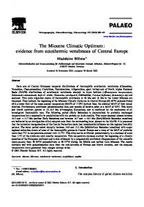
Figure 1. (a) Modern and (b) Miocene topography and bathymetry. Red triangles indicate the location of deep water temperature estimates (Table 2). L-M indicates Lago-Mare.

Tethys gateway during the Oligocene-Miocene transition lead to a reversal of Panama throughflow. [4] Micheels et al. [2011] recently used a coupled atmosphere–ocean model with reconstructed boundary conditions to examine mechanisms of heat transport in the late Miocene, focusing on atmospheric characteristics. They find that a lower-than-present northern hemisphere ocean heat transport due to weaker North Atlantic Deep Water formation is compensated by an increase in atmospheric heat transport. Thus studies not utilizing an atmosphere–ocean modeling framework may overestimate the impact of altered ocean heat transport on past or future climates. [5] In this study we use the Community Climate System Model 3 (CCSM3) to explore the effects of global Miocene

boundary conditions on ocean circulation, in comparison with a control simulation forced with modern boundary conditions. Specifically, we investigate changes in mixedlayer characteristics and water mass formation. A significant improvement over the majority of previous studies is the implementation of reconstructed physical boundary conditions (vegetation, topography and bathymetry) in a coupled atmosphere–ocean modeling framework. In this sense, the purpose of this study is to present a first order approximation of early to middle Miocene ocean circulation simulated independently of assumptions of atmospheric heat transport and surface conditions, while at the same time evaluating the ability of a well-known coupled climate model in simulating a pre-Quaternary ocean state significantly warmer than the

2 of 22

PA1209


present. A companion study examines results from the same simulations in the context of land and atmosphere climate [Herold et al., 2011].

PA1209

for analysis. We compare our Miocene case to a control case forced with modern boundary conditions and greenhouse gas concentrations appropriate for 1990, including a CO2 of 355 ppmv.

2. Model Description [6] The CCSM3 consists of four component models of the atmosphere, ocean, land and sea-ice, each communicating via a coupler [Collins et al., 2006]. Both the land and atmosphere models share a horizontal T31 spectral grid, representing a resolution of 3.75° 3.75° in longitude and latitude, respectively. The ocean model utilizes a z-coordinate system with 25 vertical levels and is configured with the GentMcWilliams scheme for eddy parameterization. Vertical mixing is handled with the KPP scheme and all tunable parameters for the mixing schemes are held at the standard, modern values used in this low resolution version of the model [Yeager et al., 2006]. The ocean and sea-ice models operate on a horizontal stretched grid of approximately 3° 1.5° in longitude and latitude, respectively, with coarser resolution at middle latitudes and finer meridional resolution at the equator. Due to numerical limitations the North Pole is centered over Greenland in the ocean and sea-ice model grids. Conservation of salinity between the atmosphere and ocean is achieved via a river transport scheme which moves excess water from land to ocean grid points according to topographic relief. The CCSM3 has been previously utilized for past [Ali and Huber, 2010; Kiehl and Shields, 2005; Liu et al., 2009; Shellito et al., 2009], present and future climate simulations [Meehl et al., 2007].

3. Experiment Design [7] For our Miocene simulation topography and bathymetry are adapted from Herold et al. [2008] (Figure 1) and vegetation is prescribed based on Wolfe [1985] with improvements based on more recent scholarship. The most important amendment is that ice is prescribed to the majority of East Antarctica. This is consistent with evidence suggesting a large ice sheet existed on the continent [Pekar and DeConto, 2006] with tundra likely occupying coastal regions [Warny et al., 2009]. N2O and CH4 are set to preindustrial concentrations of 270 ppb and 760 ppb, respectively. The solar constant is set to 1365 W/m2 (compared to 1367 W/m2 for modern CCSM3 simulations) and obliquity, eccentricity and precession are set to values appropriate for 1950. As CO2 during the Miocene is controversial [cf. Kürschner et al., 2008; Pagani et al., 1999] we prescribe a concentration of 355 ppmv, midway between the majority of estimates and the same as modern day CCSM3 simulations. This choice simplifies comparison with the modern control case. Initial ocean temperatures and salinities are based on modern global depth averages. Based on the depth-integrated ocean mean temperature the simulation equilibrates after approximately 800 years. The model is run for a further 300 years, at which point global mean ocean temperature varies by 60°N) by a shallow, intense circulation facilitated by the near-absence of the GSR (Greenland-Scotland Ridge) (Figures 5c and 5d), however, this does not reflect deep water formation. As Figure 5 represents the eularian component of the overturning circulation, a more appropriate indication of tracer transport is given by ideal-age and is discussed in the next section. [13] Gyre circulation is also less vigorous in the Miocene, particularly in the North Atlantic Ocean (Figure 6). The

largest difference between cases is the connection of the South Pacific and Indian Ocean gyres in the Miocene due to the wider Indonesian gateway. The South Atlantic and Indian Ocean gyres are weaker in the Miocene and exchange between the two oceans is reduced. This is associated with a weakening of the midlatitude westerlies and the slight southerly position of Africa in the Miocene. Simulated volume transport by the Antarctic Circumpolar Current is up to 92 Sv in the Miocene, compared to 105 Sv in the modern case (Table 1). [14] The weaker Miocene ocean circulation compared to the modern is attributed in part to a reduced meridional surface temperature gradient and consequent weakening of the southern hemisphere midlatitude westerlies (Figure 7). Substantial reductions in wind stress curl and barotropic

8 of 22


PA1209

Table 1. Volume Transport Through Gateways in Sva Gateway

Modern

Drake (zonal) Fram (meridional) Bering (meridional) Baffin Bay (meridional) Barents Sea (zonal) Panama (zonal) Tethys (zonal)

105 0.33 0.37 0.89 0.85 N/A N/A

Miocene 92 1.068 10 N/A N/A N/A 0.64 11.3

HiCO2 4

88 1.5 10 N/A N/A N/A 0.56 11.5

4

PA1209

stream function arise because of the reduction of these winds. Weakening of the North Atlantic subtropical gyre may be attributed in part to the open Panama gateway, which model sensitivity tests have shown to weaken the western boundary current [Maier-Reimer et al., 1990], however, reduced sea level pressure gradients and the associated weakening of surface winds (Figure 8) are likely the dominant forcing. Regional influences at sites of convection also influence the overturning circulation.

a

Parentheses indicate orientation of throughflow. For zonal throughflow, positive values indicate eastward flow and negative values indicate westward flow. For meridional throughflow, positive values indicate northward flow and negative values indicate southward flow.

4.4. Water Mass Formation [15] The formation of intermediate and bottom water masses and their subsequent trajectories are diagnosed using the ‘ideal age’ tracer, maximum winter boundary layer depths and velocity fields. Ideal age represents the number

Figure 7. (a) Zonal annual mean surface temperature and (b) sea-surface wind stress for the modern (blue) and Miocene cases (red). Dashed lines are Miocene minus modern anomalies with reference to right y axis. 9 of 22

PA1209


PA1209

Figure 8. Mean annual sea level pressure for the (a) modern and (b) Miocene cases.

of years water has been isolated from the sea-surface. The most significant changes between the control and Miocene cases occur in the Atlantic and thus we focus our discussion here. In the Miocene southern hemisphere significant bottom water formation is simulated in the Weddell Sea with weaker formation in the vicinity of the Ross Sea and Marie Byrd Land coast, consistent with an inferred dominant deep water source in the Southern Ocean [Wright and Miller, 1993]. Initial sinking of Weddell Sea bottom water occurs to the east, indicated by a pronounced deepening of the winter boundary layer (Figure 9b). After descending to 4,000 m Weddell Sea bottom water flows west along the PacificAntarctic ridge before turning north and east into the South Pacific and Indian Ocean basins. Accordingly bottom waters in the Pacific and Atlantic basins age northward, consistent with carbon isotope interpretations [Woodruff and Savin,

1989]. This scenario differs from the modern case where bottom water forms only weakly along the Ross Sea and Marie Byrd Land coast. This is discussed further in section 5.1. [16] Formation of proto-NADW in the Miocene (hereafter referred to as North Component Water; NCW) is simulated in the Labrador Sea; however, it is significantly weaker than its modern counterpart (Figure 10). Maximum winter boundary layer depth in the far North Atlantic is 150 m in the Miocene compared to 650 m in the modern (Figure 9). NCW descends to approximately 1,500 m, compared to approximately 3,000 m for NADW (Figure 10). No deep water formation is simulated in the Greenland-Norwegian Seas in the Miocene (Figure 9). [17] NCW is significantly warmer and more saline than NADW (Figure 11), resulting in an overall lower density. The mixed-layer in the Labrador Sea and off southeast

10 of 22

PA1209


PA1209

Figure 9. Winter time maximum boundary layer depth for the (a) modern and (b) Miocene cases. Greenland—where NADW forms in the modern case (Figure 9a)—is significantly fresher in the Miocene, contributing to the meager convection. This in turn can be explained by the relatively fresh East Greenland Current (Figure 3). Interestingly, temperature and salinity of NCW increases considerably below the mixed-layer. This is a result of exported subtropical water below the mixed-layer and is attributed to several factors. First, the Miocene subtropical gyre extends further northeastward compared to the control case (Figure 6) in association with a shift in the subtropical high pressure cell (Figure 8). We note this circulation brings Tethys outflow across the tropical North Atlantic to the Panama gateway (Figure 2b). Second, a weakening of the subpolar gyre leads to greater entrainment of northward flowing subtropical waters (Figure 6), warming the western side of the basin and NCW in the process, consistent with modern observations [Bindoff et al., 2007, pp. 396–397]. In our Miocene case this weakening is attributed to the almost absent anti-cyclonic circulation over Greenland due to a lower elevation and albedo compared to the modern (Figure 8). While subtropical water flows into the far North Atlantic in our modern simulation, mixing with the relatively stronger subpolar gyre is minimal. Finally, the

reduced deep water formation in our Miocene case reduces vertical mixing of relatively cool surface waters. Consequently, a large temperature inversion exists in the Miocene far North Atlantic compared to the modern. [18] In the Miocene case, subtropical water below the mixed-layer also enters the Greenland-Norwegian Seas and Arctic basin, along the eastern boundary. The deepest section of the GSR, which separates the Greenland-Norwegian Seas from the rest of the North Atlantic, is 4,000 m in our Miocene case and 950 m in our modern case (Figure 1). This fundamental change in circulation results in Miocene temperatures 4–5°C higher in the Greenland-Norwegian Seas and Arctic basin compared to the modern (Figure 11a), a result consistent with sensitivity tests of GSR bathymetry [Robinson et al., 2011]. [19] At approximately 1,500 m depth, NCW flows equatorward and is joined by a weak eastward Panama throughflow before continuing south as a western boundary current and mixing with the South Atlantic subtropical gyre (Figure 12). Similar southward flow occurs in the modern case however this originates from the North Atlantic subtropical gyre, which is nearly unidentifiable in the Miocene (Figure 12). Flow patterns from the tropical North Atlantic

11 of 22

PA1209


PA1209

Figure 10. Zonal mean Atlantic basin ideal age for the (a) modern and (b) Miocene cases.

to the South Atlantic are similar between the modern and Miocene cases between 1,000 and 1,500 m, above this the modern circulation shows a reversal of the boundary current in the western tropical Atlantic (to a northwesterly direction). Between 1,500 and 3,000 m, flow patterns change little in both simulations, except that velocities decrease significantly with depth in the Miocene and outflow from the Labrador Sea in the modern case starts to occur below 2,000 m. Modeled South Atlantic temperatures in the Miocene are 1–4°C above present between 300–1,500 m (Figure 11a). This relative warmth is attributed to entrainment of NCW by the South Atlantic gyre. As NCW does not descend as deeply as NADW, its southward flow does not reach the Southern Ocean. [20] The depth of the Fram Strait is 2,100 m and 1,300 m in our modern and Miocene cases respectively. Flow structure through the Fram Strait in our Miocene case is

consistent with reconstructed sea-ice migration patterns subsequent to the Miocene climatic optimum [Knies and Gaina, 2008] and is similar to the transient ‘enclosed estuarine sea’ regime proposed to have occurred during gateway widening [Jakobsson et al., 2007]. Net volume transport through the Fram Strait is southward in the modern case ( 0.33 Sv) and is balanced by flow through the Barents Sea, Bering Strait and Davis Strait (Table 1). In the Miocene case the Fram Strait is the only gateway into the Arctic basin and thus exhibits negligible net transport. 4.5. Meridional Heat Transport [21] Global ocean heat transport differs significantly in the Miocene case, with a near-symmetrical distribution about the equator (Figure 13). Peak global ocean heat transport in the Miocene southern hemisphere is up to 0.7 PW greater than modern. While temperatures in the far North Atlantic

12 of 22

PA1209


PA1209

Figure 11. Miocene minus modern (a) temperature and (b) salinity anomalies for the Atlantic basin. below the mixed-layer are significantly warmer in the Miocene case (Figure 11a) this heat is not transferred to the atmosphere, thus Miocene ocean heat transport in the far North Atlantic is less than half that of the modern (Figure 13). The majority of global heat transport change is attributable to the weakening of deep water formation in the North Atlantic and the associated disruption in ‘heat piracy’ from the southern hemisphere into the northern hemisphere. From the high northern latitudes to middle southern latitudes, changes in Atlantic heat transport are nearly directly translated onto the global heat transport budget. However, poleward of 45°S the large southward increase in Atlantic heat transport in the Miocene is compensated by a decrease in southward heat transport in the Indian Ocean (Figure 13). A shallower-than-modern Kerguelen Plateau leads to enhanced topographic steering of the Antarctic Circumpolar Current in the Miocene and a poleward shift of the subAntarctic front. The effects of this can be clearly seen in the positive temperature anomaly in Figure 2c at approximately 75°E and 45°S. The near-constancy of zonal mean heat transport poleward of 45°S is a robust feature in coupled paleoclimate modeling studies [Huber and Nof, 2006; Huber et al., 2004].

4.6. Benthic Temperature Comparison [22] Estimates of SST from planktonic foraminifera are subject to various uncertainties including assumptions of paleo-current distributions and until recently have suffered poor quality control over early diagenesis (the reader is referred to Crowley and Zachos [2000] for uncertainties regarding oxygen isotope paleothermometry). Too few wellpreserved planktonic foraminifer assemblages have been analyzed to date to make a useful comparison with modeled SSTs. Conversely, benthic foraminifera assemblages are significantly less affected by diagenesis and uncertainties in deep water pathways. Therefore we utilize published deep water temperature estimates in our model-data analysis (Table 2 and Figure 1). [23] As direct model-data comparisons do not take into account model bias we compare the warming between modern day observations and proxy records with the warming simulated between our Miocene and modern cases. The mean warming between our Miocene and modern cases across all proxy localities is 0.3°C, compared to a 4.7°C warming between proxy records and modern observations (Table 2). Thus sites of bottom water formation in our

13 of 22

PA1209


PA1209

Miocene case are significantly cooler than suggested by proxy records. This is somewhat expected considering that high latitude SSTs are cool enough to maintain considerable sea-ice formation in our Miocene case and that ice formation, the associated brine rejection and thus presumably deep water formation occur at similar temperatures compared to the present. Miocene deep water warming of the magnitude suggested by proxy records (Table 2) could only be produced by either high latitude SSTs above 0°C (either zonally or locally at sites of deep convection) or a dominant low latitude bottom water source. However, we note the cold bias in our model is overestimated by the fact that the control case is equilibrated to ‘modern’ (1990) greenhouse gases, whereas observations represent the transient response to antecedent increases in greenhouse gases. Though we speculate this has only a minor effect. [24] A direct comparison of temperatures between our modern case and modern observations reveals a mean cold bias of 0.3°C (compare modern case temperature and modern observed temperature columns in Table 2), compared to 3.5°C between our Miocene case and proxy records. This might suggest that the overwhelming majority of the model-data discrepancy is due to our Miocene boundary conditions and/or proxy records. However, it is difficult to imagine what boundary condition could produce the changes necessary to reconcile these model-data discrepancies (with the exception of CO2, see next section). The diverse range of independently formulated marine and terrestrial proxy data available in the literature also suggests with near-unanimity a globally warmer climate. Thus there are likely significant weaknesses in the sensitivity of the CCSM3, this is consistent with growing evidence that current generation GCMs, while simulating modern climates with considerable competence, are insufficiently sensitive to large magnitude climate forcings [Huber and Caballero, 2011; Valdes, 2011].

Figure 12. Temperature and velocity fields at 1,500 m depth for the (a) modern and (b) Miocene cases. Velocity reference length is 1 cm/s.

4.7. CO2 Sensitivity [25] While CO2 proxies have converged over the past decade Miocene estimates still vary by more than a factor of two [Beerling and Royer, 2011]. Given the potentially large influence of CO2 on ocean circulation an additional Miocene simulation is conducted with a CO2 concentration of 560 ppmv, twice that of the pre-industrial era. This simulation (referred to as the HiCO2 case) is branched from the standard Miocene simulation and run for 900 years to equilibrium, based on volume integrated ocean temperature. The last 100 years of output are used for analysis. Compared to the standard Miocene case, a strengthening of southern hemisphere bottom water formation, particularly in the Weddell Sea, is simulated (cf. Figures 10b and 14a). Conversely, a weakening of NCW formation occurs, with the 600 year ideal age contour approximately 300 m shallower than in the standard Miocene case. Given that the low resolution CCSM3 has a lower climate sensitivity compared with higher resolution versions of the model [Otto-Bliesner et al., 2006] and that some Miocene CO2 reconstructions are higher than 560 ppmv [Kürschner et al., 2008], higher Miocene CO2 conditions could have significantly weakened or even terminated NCW formation in our model, as has been suggested for most of the early Miocene [Woodruff and Savin, 1989].

14 of 22


PA1209

PA1209

Figure 13. Global ocean heat transport for the Miocene (red), modern (blue) and HiCO2 cases (black; see section 4.7) shown with solid lines. Miocene minus modern ocean heat transport anomalies for the Atlantic (red circles) and Indian + Pacific Oceans (red asterisks). HiCO2 minus modern ocean heat transport anomalies for the Atlantic (black circles) and Indian + Pacific Oceans (black asterisks). [26] Ocean heat transport changes in the HiCO2 case are small and occur mostly in the southern hemisphere (Figure 13). A warming of approximately 1°C occurs throughout most of the Atlantic Ocean to a depth of 500 m, though a distinct cooling in the North Atlantic occurs between 500 and 1,000 m due to reduced NCW outflow

(Figure 14b). In the Arctic, temperatures warm by 1°C at 1,000 m depth to over 2°C at the deepest level. Patterns of global zonal temperature change between the HiCO2 and standard Miocene cases are similar to the Atlantic temperature anomaly shown in Figure 14b, in that the majority of warming occurs above 1,000 m, with the exception of the

Table 2. Temperature Change Simulated by the CCSM3 Versus Temperature Change Between Modern Observations and Proxy Recordsa Simulated Simulated Modern Modern Miocene Proxy Miocene HiCO2 Warming Warming Paleo Case Observed Proxy Derived Case Case Miocene HiCO2 b d e f g Depth Paleo Temperature Temperature Temperature Case Case Temperature Temperature Warmingh c Location (m) Longitude/Latitude (°C) (°C) (°C) (°C) (°C) Referencei (°C) (°C) (°C) DSDP15 DSDP22 DSDP55 DSDP167 DSDP279 ODP747A ODP1171 DSDP573 Mean

4660 2230 3180 2910 3980 1640 1980 4390

18.5/ 29.9 31.4/ 31.3 153.9/7.6 195.7/3.4 169.5/ 53.3 75.9/ 52.2 148.9/ 54.4 121.9/ 3.4

1.0 3.3 1.4 1.8 1.1 1.3 2.5 1.0

0.9 3.4 1.9 2.3 1.4 1.7 2.6 1.7

0.9 3.4 2.3 2.7 1.7 2.3 2.9 2.0

a

0.2 0.1 0.5 0.5 0.4 0.5 0.1 0.7 0.3

0.2 0.1 0.8 0.9 0.6 1.0 0.3 0.9 0.6

2.0 2.8 1.9 1.6 1.3 2.1 3.0 1.4

6.9 6.9 6.9 6.9 6.9 7.5 6 6

4.9 4.1 5.0 5.3 5.6 5.4 3.0 4.6 4.7

1 1 1 1 2 3 4 5

To facilitate comparison between model cases and observations/proxy records, model temperatures are converted from potential to in situ temperatures based on Fofonoff and Millard [1983]. b Paleo depths calculated by adjusting for sediment load and compaction since sample deposition and by calculating subsidence since sample deposition using the GDH-1 model of Stein and Stein [1992]. c Where paleo coordinates are not provided by reference, values are calculated using modern coordinates, a plate kinematic model and the rotations of Müller et al. [2008]. d Miocene minus modern case temperature. e HiCO2 minus modern case temperature. f Levitus 1994 World Ocean Atlas (NODC_WOA94 data provided by the NOAA/OAR/ESRL PSD, Boulder, Colorado, USA, from their Web site at http://www.esrl.noaa.gov/psd/). g Where a range of values is given, the mean is used. h Miocene proxy temperature minus modern observed temperature. i References: (1) Savin et al. [1975], (2) Shackleton and Kennett [1975], (3) Billups and Schrag [2002], (4) Shevenell et al. [2008], and (5) Lear et al. [2000].

15 of 22


PA1209

PA1209

Figure 14. (a) Ideal age for the HiCO2 case and (b) the HiCO2 minus Miocene temperature anomaly for the Atlantic basin. Arctic which warms increasingly with depth. Consequently, the simulated mean warming at proxy drill locations between HiCO2 and our modern case increases only slightly (by 0.3°C; Table 2) and is still significantly less than the warming indicated by proxies. Global surface temperature in the HiCO2 case is 1.6°C warmer than the standard Miocene simulation, with maximum surface radiative warming over the Weddell Sea due to significant sea-ice reduction associated with stronger bottom water formation. Northern hemisphere annual sea-ice area decreases from 7.5 106 km2 in the standard Miocene case to 5.7 106 km2 in the HiCO2 case. In the southern hemisphere, sea-ice area decreases from 8.5 106 km2 to 5.5 106 km2. Similar to the sea-ice anomaly pattern between the standard Miocene case and the modern (Figure 4), the majority of sea-ice decrease in the HiCO2 case compared to the standard Miocene case occurs in the Weddell Sea (not shown).

5. Discussion 5.1. Deep Water Circulation [27] Our model results show fundamental circulation differences between the Miocene and modern oceans. The moderate formation of NCW in our Miocene case relative to

the present is qualitatively consistent with previous ocean models [Barron and Peterson, 1991; Bice et al., 2000; von der Heydt and Dijkstra, 2006] and various tracer data [Via and Thomas, 2006; Wright et al., 1992], though some interpretations suggest that this may be more representative of the late Miocene [Woodruff and Savin, 1989]. Conversely, Wright et al. [1992, Figures 13 and 14] infer the existence of NCW formation to depths of 3,500 m, compared to 1,500 m in our Miocene case (Figure 10). The subsequent path of NCW is also at odds with previous modeling. Nisancioglu et al. [2003] performed a series of Miocene ocean general circulation model experiments to test the sensitivity of Panama throughflow to varying sill depths. While their experiments are idealized, they show that a Panama sill depth greater than NCW outflow from the North Atlantic should drive NCW from the Atlantic to the Pacific, with an eastward surface flow. Outflow of NCW from the North Atlantic in our Miocene case occurs from approximately 1,000 m to 2,000 m and the depth of the deepest path to the Panama gateway is 1,700 m, however flow through the gateway between the mixed-layer and this depth is eastward. NCW in our Miocene case instead enters the South Atlantic as a western boundary current.

16 of 22

PA1209


[28] The warmth of Miocene NCW compared to NADW is interesting. It has been previously suggested that saline Tethys outflow increased the salinity of the North Atlantic Ocean and Greenland-Norwegian Seas, permitting the formation of relatively warm NCW [Schnitker, 1980]. Alternatively, our results suggest that NCW received its warmth and salinity below the mixed-layer due to a more northeastward orientation of the subtropical gyre and greater mixing by the sub polar gyre. Furthermore, our modeled salinities in the Tethys are not considerably different from other regions at similar latitudes. Thus, our results suggest that NCW may have been warmer and more saline than its modern counterpart without a saline Tethys outflow. Due to the coarse horizontal resolution of the CCSM3 in our study, the Strait of Gibraltar is blocked in the modern bathymetry (Figure 3a). To conserve global salinity, the CCSM3 artificially moves net freshwater fluxes from the Mediterranean Sea to the North Atlantic Ocean at the latitude of the Strait of Gibraltar, over an area of approximately 325,000 km2. A similar process in the model occurs for all seas isolated from the global ocean. While this is not ideal, it has been shown that, in comparison, explicit parameterization of the Mediterranean overflow has little effect on SSTs (