transport of hazardous waste materials through the soil surrounding a landfill .....
C.J. Geankoplis, Transport Processes and Unit Operations, Allyn and Bacon, ...
MODELING TRANSPORT PROCESSES IN HEAT AND MASS RELEASING POROUS MEDIA
by Bryan R. Becker, Ph.D., P.E. Associate Professor Mechanical and Aerospace Engineering Department and Brian A. Fricke Research Assistant Mechanical and Aerospace Engineering Department
University of Missouri-Kansas City 5605 Troost Avenue Kansas City, MO 64110-2823 U.S.A.
26 August 1996
MODELING TRANSPORT PROCESSES IN HEAT AND MASS RELEASING POROUS MEDIA
Bryan R. Becker, Ph.D., P.E. and Brian A. Fricke University of Missouri-Kansas City Department of Mechanical and Aerospace Engineering 5605 Troost Avenue, Kansas City, MO 64110-2823, U.S.A.
ABSTRACT A computer algorithm was developed which estimates the latent and sensible heat loads due to the heating or cooling of heat and moisture releasing porous media. The algorithm also predicts the moisture loss and temperature distribution which occurs during the heating or cooling process. This paper discusses the modeling methodology utilized in the current computer algorithm and describes the development of the heat and mass transfer models. The results of the computer algorithm are compared to experimental data taken from the literature.
Introduction Many important applications make use of heat and mass transfer in porous media. The aqueous transport of hazardous waste materials through the soil surrounding a landfill site can be simulated with porous media analysis [1]. Porous media analysis can also be used to model the heat and mass transfer which occurs during the storage of agricultural products such as fruits, vegetables and grains [2-8]. In addition, the drying of rice and grain can be modeled as porous media flows [9]. In HVAC applications, a porous, moisture absorbing material can be used to dehumidify air [10, 11], while in the textile, wood and paper products industries, various processes are used for the drying of porous, manufactured materials [1215]. Estimates of the heat and mass transfer within a porous medium are important to the designers of commodity storage facilities, as well as the designers of various drying and dehumidifying processes. These estimates require knowledge of the complex interaction of the various thermophysical processes which occur within and around the materials which compose the porous medium. Therefore, a computer algorithm was developed to simulate the heat and mass transfer which occurs within a heat and moisture releasing porous medium. The combined phenomena of heat and mass release, air flow, and convective heat and mass
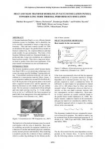
transfer are included in the model. In this paper, the modeling methodology utilized in this computer algorithm is described and the results of the computer model are compared to experimental data taken from the literature. A review of the literature has revealed several existing models of the heat transfer in the heating or cooling of porous media [2-8, 13, 14, 16-18]. However, none of these models provide a thorough treatment of the combined phenomena of moisture loss, heat generation and temperature gradient within the porous medium. Therefore, the current computer algorithm was developed to estimate the latent and sensible heat loads as well as the moisture loss and temperature distribution which occurs during the heating or cooling of heat and moisture releasing porous media. Modeling Methodology As depicted in Figure 1, the computational model is based upon a one dimensional air flow pattern within a bulk load of heat and moisture releasing spherical shaped objects, hereafter referred to as "commodities." In the computational model, the bulk load is represented as a porous medium composed of "commodity computational cells." The conditioned air is modeled as "air parcels" which move through the "commodity computational cells."
FIG. 1 Computational model of refrigerated air flow through bulk load of commodity. Calculation commences with a specified initial temperature and humidity for the bulk load and the air contained within it. As shown in Figure 1a, the time-stepping begins with the first refrigerated "air parcel" moving into the first "commodity computational cell." At the same time, each of the initial "air parcels" moves from its original cell into the adjacent cell, while the "air parcel" within the last "commodity
computational cell" moves from the bulk load into the plenum of the refrigeration unit. Within each
& 1, is calculated for the time-step, ?t. The "commodity computational cell," the moisture release rate, m mass fraction of water vapor in each "air parcel" is then updated to reflect the effects of moisture release. Subsequently, within each cell, the heat generation, W, the heat transfer from the commodity, Q, and the evaporative cooling due to moisture release are calculated for the time-step. Then, within each cell, the porous medium temperature and the "air parcel" temperature are both updated to reflect the effects of heat generation, heat transfer and evaporative cooling, thus completing the calculations for this time-step. As shown in Figure 1b, the first "air parcel" moves to the second "commodity computational cell" and a newly conditioned second "air parcel" moves into the first "commodity computational cell." This second "air parcel" encounters the previously updated porous medium temperature in the first "commodity computational cell." As the time-stepping continues, each "air parcel" traverses the entire bulk load. The mass fraction of water vapor contained in each "air parcel," when it exits the bulk load, is used to calculate the latent heat load corresponding to that "air parcel," while its temperature is used to calculate its sensible heat load. As this algorithm time-steps towards a steady state, an estimate of the time histories of the latent and sensible heat loads, as well as moisture loss and temperature distribution, are obtained.
Mass Transfer Calculation Transpiration is the moisture loss process which includes the transport of moisture through the thin, porous skin of the commodity, the evaporation of this moisture from the commodity surface and the convective mass transport of the moisture to the surroundings. The driving force for transpiration is a difference in water vapor pressure between the surface of the commodity and the surrounding air. Hence, the moisture loss from a single commodity is modeled as follows:
& = k t ( Ps - P a ) m
(1)
where kt is the transpiration coefficient, Ps is the water vapor pressure at the surface of the commodity and Pa is the water vapor pressure in the air. It is assumed that the water vapor pressure at the surface of the commodity, Ps , is equal to the water vapor saturation pressure evaluated at the commodity surface temperature. The water pressure in the air, Pa , is a function of the mass fraction of water vapor in the air. Both Ps and Pa are evaluated at the previous time step by utilizing psychrometric relationships [19]. Fockens and Meffert [20] suggest that the transpiration coefficient, kt , can be modeled as follows:
1 kt = 1 1 + ka ks
(2)
where ka is the air film mass transfer coefficient and ks is the skin mass transfer coefficient. The air film mass transfer coefficient, ka , describes the convective mass transfer which occurs at the surface of the commodity and can be calculated via the Sherwood number, Sh, as follows:
Sh = k a δ
d
(3)
where d is the diameter of the commodity and d is the diffusion coefficient of water vapor in air. The following Sherwood-Reynolds-Schmidt correlation from Geankoplis [21] can be used to determine the convective mass transfer from a sphere:
Sh = 2.0 + 0.552 Re0.53 Sc0.33
(4)
where Re is the Reynolds number and Sc is the Schmidt number. The skin mass transfer coefficient, ks , describes the skin's diffusional resistance to moisture migration and is dependent upon the fraction of the commodity surface covered by pores. As such, it is theoretically difficult to determine the skin mass transfer coefficient, and thus, ks must be determined experimentally. For example, Chau et al. [22] and Gan and Woods [5] have experimentally determined the skin mass transfer coefficient for various fruits and vegetables. During the time step, ?t, the mass of water vapor in the air of the computational cell increases as follows:
&t∆t mH 2 O1 = mH 2 O0 + m
(5)
where mH2O1 is the updated mass of water vapor in the air, mH2O0 is the mass of water vapor in the air from & t 7 is the transpiration rate in the computational cell and ?t is the time step size. the previous time step, m The updated mass fraction of water vapor in the air of the computational cell, mf1, then becomes: 1
m1f =
mH 2 O 0 &t ∆t ma + m
(6)
where ma0 is the mass of air within the computational cell. With the updated mass fraction of water vapor in the air, the relative humidity within the computational cell may be determined via psychrometric relationships. This completes the transpiration calculations for one computational cell for the current time step. Heat Transfer Calculation In order to make the modeling of heat transfer tractable, the porous medium was assumed to consist of spheres with uniform internal heat generation. It was further assumed that the temperature within a commodity varied only in the radial direction. With these assumptions, the governing form of the transient heat equation is formally written as follows [23]:
k ∂ 2 ∂T ∂T r + ρ W= ρc 2 ∂t r ∂r ∂r
(7)
where r denotes the radial direction, k is the thermal conductivity, T is the temperature, W is the heat
generation per unit mass, ? is the density, c is the specific heat, and t is time. An explicit finite difference technique was applied to Equation (7) by dividing a commodity into N spherical shells. The resulting finite difference equation applicable to the center node is given as follows:
k A1 0 0 ρ c v1 ( T11 - T01 ) ( T 2 - T1 ) + ρ v1 W1 = ∆r ∆t
(8)
The resulting finite difference equation applicable to the interior nodes is given as follows:
k A i - 1 ( Ti0 - 1 - T 0i ) k A i ( T i0 + 1 - T0i ) ρ c v i ( T1i - T0i ) + + ρ v i Wi = ∆r ∆r ∆t
(9)
At the surface of the commodity, convection heat transfer, radiation heat transfer, and evaporative cooling due to transpiration must be considered. Thus, the finite difference equation at the surface becomes:
k A N-1 0 ρ c v N ( T1N - T 0N ) & As + ρ v N W N = ( T N - 1 - T0N ) + heff As ( T0a - T 0N ) - Lm ∆r ∆t
(10)
The effective heat transfer coefficient, heff , includes both convection and radiation:
heff = hconvection + h radiation
(11)
The convection heat transfer coefficient, hconvection , in Equation (11) is obtained from the Nusselt number, Nu, as follows:
Nu = h convection kair
d
(12)
where d is the diameter of the commodity and kair is the thermal conductivity of air. The convective heat transfer is determined via the Nusselt-Reynolds-Prandtl correlation given by Geankoplis [21]:
Nu = 2.0 + 0.552 Re0.53 Pr 0.33
(13)
where Pr is the Prandtl number. The radiation heat transfer coefficient, hradiation , in Equation (11) is given by:
2 2 h radiation = σ ( Ts + T a ) ( Ts + Ta )
(14)
where Ts is the commodity surface temperature, Ta is the air temperature and s is the Stefan-Boltzmann constant. The formulation given by Equations (8), (9) and (10) defines the temperature distribution within a single commodity. However, Equation (10) requires knowledge of the temperature of the air parcel resident within the "commodity computational cell," Ta0. This air temperature is determined at each time step by performing a heat balance between the air parcel and that portion of the bulk load which is contained within the "commodity computational cell:" 0 0 0 nc heff A s ( T a - T N ) = ma cp,a
( T1a - T 0a ) ∆t
(15)
where nc is the number of commodities resident within the "commodity computational cell," ma0 is the mass of air in the computational cell and cp,a is the specific heat of air. This completes the formulation of the heat
transfer model for one computational cell. Since Equations (8), (9), (10) and (15) are explicit finite difference equations, they can be solved directly for the updated nodal temperatures. The heat transfer calculation begins at the center node of the commodity and proceeds outward to the air parcel. This completes the heat transfer calculation for one computational cell for the current time step. Experimental Verification of the Computer Algorithm To verify the accuracy of the current computer algorithm, its calculated results were compared with experimental data on the bulk refrigeration of fruits and vegetables, obtained from the literature. Baird and Gaffney [3] reported experimental data taken from bulk loads of oranges. They recorded commodity center and surface temperatures at the air exit of a bulk load for a period of two hours. The bulk load of oranges was 0.67 m (2.2 ft) deep and the commodities were initially at 32°C (90°F). The refrigerated air was at a temperature of -1.1°C (30°F) and approached the bulk load with a velocity of 0.91 m/s (3.0 ft/s). Figure 2 shows Baird and Gaffney's experimental data along with the output from the current computer algorithm. Comparison of the model results with Baird and Gaffney's data on oranges shows that the current algorithm correctly predicts the trends of commodity temperatures with a maximum error of 1.4°C (2.5°F).
FIG. 2 Current numerical results and experimental temperature data for forced air cooling of oranges from Baird and Gaffney (1976).
Brusewitz et al. [24] conducted experiments to determine moisture loss from peaches during postharvest cooling.
The post-harvest cooling was performed at 4°C (39°F), 92% relative humidity in a
chamber with 20 air changes per minute for a period of four days. Peaches were picked in the morning when the ambient temperature was 16°C (61°F). Experimental data from Brusewitz et al. shows that the peaches lost 2.5% of their weight due to moisture loss during the four day cooling period. The current computer algorithm predicted a weight loss of 2.53% at the end of the four day period, in good agreement with the experimental data. Figure 3 shows the results from the current computer algorithm as well as the experimental data.
FIG. 3 Current numerical results and experimental moisture loss data for post harvest cooling of peaches from Brusewitz et al. (1992).
Conclusions This paper has described the development and performance of a computer algorithm which estimates the latent and sensible heat loads as well as the moisture loss and temperature distribution within a bulk load of heat and moisture releasing, spherical commodities. In the computational model, the bulk load is represented as a porous medium composed of "commodity computational cells" and the conditioned air is modeled as "air parcels" which move through these "commodity computational cells." A mass transfer model was developed to update the mass fraction of water vapor within each "commodity computational cell" at each time step. An explicit finite difference formulation of the transient heat equation in spherical
coordinates was derived which accounts for both radiation and convection heat transfer at the commodity surface.
This formulation yields the temperature distribution within the commodities resident in each
"commodity computational cell" at each time step. It also yields the temperature of the "air parcel" resident within each "commodity computational cell" at each time step. To verify the accuracy of the current algorithm, its calculated results were compared with experimental data obtained from the literature. The results of these comparisons show good agreement between the numerical results and the experimental data for both temperature and moisture loss. Nomenclature Ai As A1 c cp,a d hconvection heff hradiation k ka kair ks kt L ma0 mf1 mH2O0 mH2O1
m& m& t
nc N Nu Pa Ps Pr Q r Re Sc Sh t T Ta Ta0 Ta1 Ti0
surface area of ith node single commodity surface area surface area of center node specific heat of commodity specific heat of air diameter of commodity convection heat transfer coefficient effective heat transfer coefficient radiation heat transfer coefficient thermal conductivity of commodity air film mass transfer coefficient thermal conductivity of air skin mass transfer coefficient transpiration coefficient latent heat of vaporization of water mass of air at time t mass fraction of water vapor in air at time t + ?t mass of water vapor in air at time t mass of water vapor in air at time t + ?t transpiration rate per unit area of commodity surface transpiration rate in computational cell number of commodities in computational cell number of nodes Nusselt number ambient water vapor pressure water vapor pressure at evaporating surface of commodity Prandtl number heat transfer commodity radius Reynolds number Schmidt number Sherwood number time commodity temperature dry bulb air temperature air temperature at time t air temperature at time t + ?t temperature of ith node at time t
Ti1 TN0 TN1 Ts T10 T11 vi vN v1 W Wi WN W1 d ?r ?t ? s
temperature of ith node at time t + ?t temperature of surface node at time t temperature of surface node at time t + ?t product surface temperature temperature of center node at time t temperature of center node at time t + ?t volume of ith node volume of surface node volume of center node rate of heat generation of commodity per unit mass of commodity rate of heat generation of commodity per unit mass of commodity for node i rate of heat generation of commodity per unit mass of commodity for surface node rate of heat generation of commodity per unit mass of commodity for center node coefficient of diffusion of water vapor in air length of node in radial direction time step size density of commodity Stefan-Boltzmann constant References
1.
P.J. Hensley and A.N. Schofield, Accelerated Physical Modelling of Hazardous-Waste Transport, Geotechnique, 41(3), 447 (1991).
2.
F.W. Bakker-Arkema and W.G. Bickert, A Deep-Bed Computational Cooling Procedure for Biological Products, Transactions of the ASAE, 9(6), 834 (1966).
3.
C.D. Baird and J.J. Gaffney, A Numerical Procedure for Calculating Heat Transfer in Bulk Loads of Fruits or Vegetables, ASHRAE Transactions, 82(2), 525 (1976).
4.
N. Adre and M.L. Hellickson, Simulation of the Transient Refrigeration Load in a Cold Storage for Apples and Pears, Transactions of the ASAE, 32(3), 1038 (1989).
5.
G. Gan and J.L. Woods, A Deep Bed Simulation of Vegetable Cooling, In Agricultural Engineering, ed. V.A. Dodd and P.M. Grace, p. 2301, A.A. Balkema, Rotterdam (1989).
6.
W.E. Stewart, Jr., M.E. Greer, L.A. Stickler and B.R. Becker, Heat Transfer in Partial Underground Cold Storage of Grain, Joint ASME/AIChE National Heat Transfer Conference, August 5-8, 1989, Philadelphia, PA, ASME, New York (1989).
7.
M.T. Talbot, C.C. Oliver and J.J. Gaffney, Pressure and Velocity Distribution for Air Flow Through Fruits Packed in Shipping Containers Using Porous Media Flow Analysis, ASHRAE Transactions, 96(1), 406 (1990).
8.
I.R. MacKinnon and W.K. Bilanski, Heat and Mass Transfer Characteristics of Fruits and Vegetables Prior to Shipment, SAE Technical Paper 921620, SAE, Warrendale, PA (1992).
9.
A.H. Zahed and N. Epstein, On the Diffusion Mechanism During Spouted Bed Drying of Cereal Grains, Drying Technology, 11(2), 401 (1993).
10.
D. Balkose, H. Baltacioglu and F. Abugaliye, Drying of Air in Silica Gel Packed Columns, Drying Technology, 8(2), 367 (1990).
11.
A. Ertas, E.E. Anderson and S. Kavasogullari, Comparison of Mass and Heat Transfer Coefficients of Liquid-Desiccant Mixtures in a Packed Column, Journal of Energy Resource Technology, Transactions of the ASME, 113(1), 1 (1991).
12.
S.H. Lin, Moisture Desorption in Cellulosic Materials, Industrial Engineering Chemical Research, 30(8), 1833 (1991).
13.
J.Y. Liu, Drying of Porous Materials in a Medium With Potentials Varying Exponentially With Time, ASME/JSME Thermal Engineering Joint Conference Proceedings 3, p. 315, ASME, New York (1991).
14.
J.Y. Liu, Zonal Analysis of Heat and Mass Transfer in the Drying of Porous Media, Convective Heat Transfer and Transport Process - 1991 ASME Heat Transfer Division, p. 35, ASME, New York (1991).
15.
M. Can and E. Pulat, Investigation into Drying of Fabrics as a Flat Porous Structure, Proceedings of the 1992 Engineering Systems Design and Analysis Conference, June 29 to July 3, 1992, Istanbul, Turkey, p. 81, ASME, New York (1992).
16.
C. Appert, A. Melayah, V. Pot, D.H. Rothman and S. Zaleski, Simulating Evaporation in Porous Media with the Lattice Gas Method, Proceedings of the 9th International Conference on Computational Methods in Water Resources, June 1992, Denver CO, p. 409, Computational Mechanics Publishers, Southampton, England (1992).
17.
S.C. Nowicki, H.T. Davis and L.E. Scriven, Microscopic Determination of Transport Parameters in Drying Porous Media, Drying Technology, 10(4), 925 (1992).
18.
J. Irudayaraj, K. Haghighi and R.L. Stroshine, Nonlinear Finite Element Analysis of Coupled Heat and Mass Transfer Problems with an Application to Timber Drying, Drying Technology, 8(4), 731 (1990).
19.
ASHRAE, Brochure on Psychrometry, ASHRAE, Atlanta, GA (1970).
20.
F.H. Fockens and H.F.T. Meffert, Biophysical Properties of Horticultural Products as Related to Loss of Moisture During Cooling Down, Journal of the Science of Food and Agriculture, 23, 285 (1972).
21.
C.J. Geankoplis, Transport Processes and Unit Operations, Allyn and Bacon, Boston (1978).
22.
K.V. Chau, R.A. Romero, C.D. Baird and J.J. Gaffney, Transpiration Coefficients of Fruits and Vegetables in Refrigerated Storage, ASHRAE Report 370-RP, ASHRAE, Atlanta (1987).
23.
F.P. Incropera and D.P. DeWitt, Fundamentals of Heat and Mass Transfer, John Wiley and Sons, New York (1990).
24.
G.H. Brusewitz, X. Zhang and M.W. Smith, Picking Time and Postharvest Cooling Effects on Peach Weight Loss, Impact Parameters, and Bruising, Applied Engineering in Agriculture, 8(1), 84 (1992).